Alternative Ef
Þ
ciency Measures for
Multiple-Output Production
Carmen Fern´andez
Department of Mathematics and Statistics, Lancaster University, Lancaster, LA1 4YF, U.K.
Gary Koop
Department of Economics, University of Leicester, Leicester, LE1 7RH, U.K.
Mark Steel∗
Department of Statistics, University of Warwick, Coventry, CV4 7AL, U.K.
August 2003
This paper has two main purposes. Firstly, we develop various ways of defining efficiency in the case of multiple-output production. Our frame-work extends a previous model by allowing for nonseparability of inputs and outputs. We also specifically consider the case where some of the outputs are undesirable, such as pollutants. We investigate how these effi-ciency definitions relate to one another and to other approaches proposed in the literature. Secondly, we examine the behavior of these definitions in two examples of practically relevant size and complexity. One of these involves banking and the other agricultural data. Our findings are basi-cally encouraging. For a given efficiency definition, efficiency rankings are found to be informative, despite the considerable uncertainty in the infer-ence on efficiencies. It is, however, important for the researcher to select an efficiency concept appropriate to the particular issue under study, since different efficiency definitions can lead to quite different conclusions.
Keywords: banking, Bayesian inference, dairy farms, pollution, productivity, separability
JEL classiÞcation: C11, D24
1
Introduction
The evaluation of the efÞciency of individualÞrms is of fundamental importance for
policymak-ing in many areas of economics. Stochastic frontier models have been one of the most popular
tools for carrying out such efÞciency analyses. Numerous applications in the Þelds ofÞnance
(e.g. Hunt-McCool, Koh and Francis, 1996), banking (e.g. Adams, Berger and Sickles, 1999,
Fern´andez, Koop and Steel, 2000), agriculture (e.g.Kumbhakar, Ghosh and McGuckin, 1991),
environmental economics (e.g. Reinhard, Lovell and Thijssen, 1999), public sector economics
(e.g.Perelman and Pestieau, 1994) and development economics (e.g.Pitt and Lee, 1981) testify
to the importance economists in diverse applied Þelds place on efÞciency measurement.
How-ever, researchers must be cautious when usingÞrm-speciÞc efÞciency measures to rankÞrms or
make statements about whether a Þrm is more or less efÞcient than others. The necessity for
caution arises for two reasons. Firstly, Þrm-speciÞc efÞciency is typically hard to estimate and
associated measures of uncertainty (e.g.conÞdence intervals or Bayesian posterior standard
devi-ations) can be quite large. Merely looking at point estimates can potentially be very misleading.
Secondly, there is not one unique deÞnition of efÞciency and aÞrm which is ranked as being very
efÞcient using one deÞnition could potentially be ranked quite differently using another. The
latter problem is exacerbated in the case of multiple-output production which forms the basis of
the present paper.
These considerations motivate the focus of this paper. In particular, we develop and discuss
several deÞnitions of efÞciency for the case of multiple-output production. We allow for
non-separability of inputs and outputs by making the elasticity of transformation between outputs a
parametric function of the inputs. We also treat the case where some of the outputs produced
might be undesirable by-products of the production process, such as pollution. We shall use
Bayesian methods for making inference aboutÞrm-speciÞc efÞciency using these deÞnitions and
compare the resulting efÞciency rankings and conclusions in the context of two applications. We
consider the empirically relevant case where the researcher only has data on inputs and outputs.
That is, data on input or output prices, costs or proÞts are not available. Of course, if some or
all of these were available, the problems involved in multiple-output production would be greatly
simpliÞed. For instance, if a cost function could be estimated, then outputs could be included as
explanatory variables with cost being the dependent variable. However, this would not allow the
development and analysis of a variety of output-oriented efÞciency measures, each of which can
Bayesian inference produces exact Þnite-sample posterior and predictive distributions and
fully takes parameter uncertainty into account. It was found in previous work (seee.g. Koop,
Osiewalski and Steel, 1994, 1997) to be an excellent tool for inference on efÞciencies in stochastic
frontier models, allowinge.g.for economic regularity conditions to be imposed in a very simple
way. See Kim and Schmidt (2000) for some empirical comparisons of Bayesian and classical
approaches to efÞciency measurement.
TheÞrst of the empirical applications is on the banking data of Adamset al.(1999), also used
in Fern´andezet al.(2000). The second is the environmental application of Reinhardet al.(1999)
and Fern´andez, Koop and Steel (2002). OurÞndings indicate that, given an efÞciency deÞnition,
efÞciency rankings do have some practical relevance, despite the considerable uncertainty in
the inference on efÞciencies. On the other hand, it is critical that we focus on the appropriate
efÞciency concept for the particular purpose at hand, since different efÞciency deÞnitions can
lead to quite different conclusions, both in terms of rankings and absolute values. The paper is
organized as follows: In the second section we introduce our multiple-output production model.
The third section discusses the issue of efÞciency measurement in this model. The fourth section
discusses some related approaches in the literature. Section 5 presents our two applications and
the sixth concludes. Details on the prior adopted and the Markov chain Monte Carlo (MCMC)
sampler used to conduct inference are given in the Appendix.
2
The Model
The best-practice technology for producing a vector of outputs,y, from a vector of inputs,x, can
be described using a transformation function:
f(y, x) = 0.
In this paper we shall assume the transformation function has the form:
g(y, x) =h(x),
with a particular class of functions g(y, x). The left and right hand sides of this equation are referred to as the aggregate output and production frontier, respectively. In the present paper, we
adopt a modiÞcation of the setup of Fern´andezet al.(2000), hereafter FKS. As we shall see, our
particular choice for the transformation function allows freeing up the separability assumption of
We consider a set of NT observations corresponding to outputs of N different Þrms (or
agents) whereÞrmiis observed forTitime periods. Note that this accommodates an unbalanced
panel. For a balanced panel, we will have Ti = T, i = 1, . . . , N. Generally, however, T will be deÞned as(T1 +· · ·+TN)/N. The output ofÞrmi(i = 1, . . . , N) at timet(t = 1, . . . , Ti) is a p-dimensional vectory(i,t) = (y(i,t,1), . . . , y(i,t,p))′ ∈ ℜp+, and we assume that the aggregate
output can be expressed as:
g(y(i,t), x(i,t)) =
p
j=1
αq(x(i,t))
j y
q(x(i,t))
(i,t,j)
1/q(xi,t)
, (1)
whereα = (α1, . . . , αp)′ withαj ∈ (0,1)for allj = 1, . . . , pandpj=1αj = 1. In addition, we assume thatq(x(i,t)) > 1is a function of the inputsx(i,t) corresponding to Þrmiat timet given
by:
q(x(i,t)) = (1 +ψ0)
m
l=1
(1 +ψl)x(i,t,l), (2)
whereψ = (ψ0, . . . , ψm)′is a parameter vector inℜ+m+1andx(i,t,l) is thelth input corresponding
to observation(i, t). To avoid cluttering the notation, we will not explicitly indicate the depen-dence of the output aggregatorg(·,·)in (1) onαandq(x(i,t)). ForÞxed values ofαandq(x(i,t)),
g(y(i,t), x(i,t)) = constant deÞnes a production equivalence surface, i.e.a (p−1)-dimensional
surface in ℜp+ consisting of all output vectors y(i,t) that are technologically equivalent. The
ag-gregation function used in (1) has been used in Powell and Gruen (1968) and Kumbhakar (1987)
and is sometimes called the “constant elasticity of transformation” aggregator, since it imposes
the same elasticity of transformation between any two outputs. This elasticity of transformation
is given by{1−q(x(i,t))}−1, which explains the restrictionq(x(i,t))>1as this ensures a negative
elasticity of transformation and also shows that this elasticity can be inßuenced by the input
val-ues. Thus, we have not imposed separability between inputs and outputs, and it is exactly through
the most interesting property of the aggregator function that we allow forx(i,t) to intervene. The
interpretation of the parameterαin (1) is to deal with scaling of the outputs, which is, therefore,
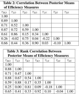
quite separate from the role ofq(x(i,t)). Figure 1a illustrates the latter by displaying the range of
production equivalence surfaces corresponding to various values ofq(x(i,t)). With given inputs in
h(x(i,t)), the production possibility set clearly increases with the value ofq(x(i,t)). In the special
case of separability whereq(x(i,t)) =qand givenq, the regularity conditions onh(x(i,t))would
imply a reduction of the production possibility set for smaller inputsx(i,t) (monotonicity). If in
our more general separable framework we would allow for q(x(i,t))to be strictly decreasing in
produc-tion possibility set which is not strictly contained in the old one1. In order to make sure that
monotonicity in inputs holds for our nonseparable model, the speciÞcation in (2) imposes that
q(x(i,t))is a nondecreasing function of the inputs.
FKS use the transformation function in (1) with q(x(i,t)) = q. The latter assumption
cor-responds to ψl = 0, l = 1, . . . , m and, thus, imposes the special case of separability in inputs and outputs of the production technology. As indicated by two Referees, this is a potentially
restrictive assumption, so the present paper allows for nonseparability. We shall comment on the
empirical support for this separability assumption in the context of our two applications in
Sec-tion 5. In these applicaSec-tions, we shall use the levels of all inputs in (2), standardized to be in the
interval [0,1]by subtracting the maximum value in the sample. The latter helps in interpreting values for the coefÞcientsψ1, . . . , ψmand makes a common prior (see (A.7) in the Appendix) a
reasonable assumption.
Since the aggregate outputg(y(i,t), x(i,t))is a univariate quantity, it is natural to model it using
a single-output stochastic frontier speciÞcation. To this end we deÞneδ(i,t) = log(g(y(i,t), x(i,t))),
group these transformed outputs in anNT-dimensional vector
δ = (δ(1,1), δ(1,2), . . . , δ(1,T1), . . . , δ(N,TN))
′, (3)
and modelδas
δ=V β−γ+ε. (4)
In the latter equation,V = (v(x(1,1)), . . . , v(x(N,TN)))
′ denotes anNT ×kmatrix of exogenous
regressors, wherev(x(i,t))is ak-dimensional function of the inputsx(i,t). The particular choice
of v(·)deÞnes the speciÞcation of the production frontier: e.g.the vector v(x(i,t))contains a 1
and all logged inputs for a Cobb-Douglas technology, whereas a translog frontier also involves
squares and cross products of these logs. The corresponding vector of regression coefÞcients is
denoted byβ ∈ B ⊆ ℜk. Often, theoretical considerations will lead to regularity conditions on
β, which will restrict the parameter space Bto a subset of ℜk, stillk-dimensional and possibly depending onx. For instance, we typically want to ensure that the marginal products of inputs
are positive. Such conditions are easy to impose through the MCMC sampler described in the
Appendix.
Technological inefÞciency is captured by the fact that Þrms may lie below the frontier, thus
leading to a vector of deviations between (the log of) actual and maximum possible aggregate
1The production equivalence surface would shift towards the origin close to the axes in Figure 1a, due to the
reduction inh(x(i,t)), but this could be more than offset by an outward shift of the surface for roughly equal values
output. This vector of deviations is labelledγ. It is usually reasonable to place some additional
structure on these deviations. In particular, we setγ≡Dz ∈ ℜN T
+ , whereDis a ÞxedNT ×M
(M ≤ NT) matrix and z ∈ Z with Z = {z = (z1, . . . , zM)′ ∈ ℜM : Dz ∈ ℜN T+ }. Through
different choices of D, we can accommodate various amounts of structure on the vector γ of
inefÞciencies. For instance, taking D = IN T, the NT-dimensional identity matrix, leads to an inefÞciency term which is speciÞc to each different Þrm and time period. For a balanced
panel, choosing D = IN ⊗ιT, where ιT is aT-dimensional vector of ones and ⊗denotes the Kronecker product, implies inefÞciency terms which are speciÞc to eachÞrm, but constant over
time (i.e.“individual effects”). In our empirical section we make the latter choice forD, but with
the obvious extension to unbalanced panels for our second application. Fern´andez, Osiewalski
and Steel (1997) provides a detailed description of other possible choices for D. In the next
section, we will provide deÞnitions of efÞciency which will all be functions of this deviationγ.
In previous work (see van den Broeck, Koop, Osiewalski and Steel, 1994), it was found that a
reasonable choice for the distribution ofzis a product of conditionally independent Exponentials.
See the Appendix for more details.
The model in (4) also includes a two-sided error term ε which captures the fact that the frontier is not known exactly, but needs to be estimated from the data. We assume thatεfollows
anNT-dimensional Normal distribution with zero mean and covariance matrix equal toσ2I
N T.
Hence, we obtain:
p(δ|β, z, σ) = fNN T(δ|V β−Dz, σ2IN T), (5)
wherefN T
N (.|a, A)denotes theNT-variate Normal density function with meanaand covariance matrixA.
As discussed in FKS, the previous assumptions are not enough to specify the likelihood
func-tion. Intuitively, a single equation as in (5) is not sufÞcient to determine a probability density
function for thep-dimensional vectory(i,t)ifp > 1. Hence, stochastics for thep−1remaining
dimensions must be speciÞed by considering the distribution of the outputs within each of the
production equivalence surfaces. DeÞning
η(i,t,j) =
αq(x(i,t))
j y
q(x(i,t))
(i,t,j)
p
l=1α
q(x(i,t))
l y
q(x(i,t))
(i,t,l)
, j = 1, . . . , p, andη(i,t) = (η(i,t,1), . . . , η(i,t,p))′, (6)
we assume independent sampling across observational units (for i = 1, . . . , N; t = 1, . . . , Ti) from
wheres= (s1, . . . , sp)′ ∈ ℜp+andfp
−1
D (η|s)denotes the p.d.f. of a(p−1)-dimensional Dirichlet distribution with parameters(see Poirier, 1995, page 132). From (6) we see thatη(i,t)can loosely
be interpreted as a vector of output shares, with 0 ≤ η(i,t,j) ≤ 1 and pj=1η(i,t,j) = 1. The
Dirichlet distribution is a veryßexible distribution commonly used to model shares.
The Appendix provides details regarding the prior distribution for all the parameters in the
model. The posterior obtained from combining the prior with the likelihood function is not
analytically tractable, but an MCMC algorithm can be developed to produce random draws from
the posterior. These draws can then be used to obtain posterior properties for all of the efÞciency
measures. Details of the MCMC sampler are also brießy described in the Appendix.
3
Ef
Þ
ciency Measures
The previous section outlined an econometric model for multiple-output production where
sepa-rability is not imposed and inefÞciency is possible. If we focus on a single observation, and drop
the(i, t)subscript from all variables for convenience, equation (4) can be written as:
g(y, x) = h(x)e−γeε, (8)
whereh(x)is the production frontier [i.e.exp{v(x)′β}]. Note that we do not explicitly indicate
the dependence ofg(·,·)onαandq(x), and ofh(·)onβ. In order to derive explicit measures of efÞciency, we relate the model in (8) to various efÞciency concepts.
3.1
Radial Output-Oriented Ef
Þ
ciency
The most common measure of efÞciency is known as radial output-oriented technical efÞciency,
τRO. The inverse of this (i.e.1/τRO) measures the amount by which allpoutputs must be
propor-tionally increased in order to get to the frontier. Clearly, for an inefÞcientÞrm we obtainτRO <1, whereasτRO = 1corresponds to full efÞciency.
The (stochastic) frontier faced by the Þrm with inputs xis given by h(x)eε. Hence, radial output-oriented efÞciency is deÞned by the equation
g
y1
τRO
, . . . , yp τRO
, x
=h(x)eε, (9)
where 0 < τRO ≤ 1and is equal to the output-distance function (see Shephard, 1970, or F¨are and Primont, 1995) mentioned in some detail in Section 4. We can use (8) and (9) and the
homogeneity ofg(y, x)in (1) to obtain:
This is the deÞnition of efÞciency used in FKS. Note that the individual effects structure ofγwill
be inherited by τRO, so that eachÞrm will be assumed to have a speciÞc radial output-oriented
efÞciency constant over time.
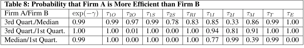
Radial output-oriented efÞciency is illustrated in Figure 1b. ThisÞgure plots the production
equivalence surface corresponding to the frontier (for a given level of inputs) for the two output
case withq(x) = 1.5. In other words, for a given level of inputs, the possible output combina-tions that are achievable by a fully efÞcientÞrm are mapped out. If a Þrm using those inputs is
producing at point A, its radial output-oriented efÞciency is given byτRO =|OA|/|OB|.
3.2
Individual Output-Oriented Ef
Þ
ciencies
In some cases, radial output-oriented efÞciency, with its focus on a proportionate increase in all
outputs, may not be the sensible efÞciency measure. For instance, a bank may be interested in
how much it can increase real estate loans, without affecting output of commercial loans. In this
case, interest centers on the potential increase in one particular output and measures of individual
output-oriented efÞciencies, say,τjO forj = 1, . . . , p, are called for. Formally, 1/τjOmeasures the amount by which output j must proportionally be increased in order to get to the frontier.
Reasoning as in the previous subsection,τjO is thus deÞned by:
g
y1, . . . ,
yj
τjO
, . . . , yp, x
=h(x)eε. (11)
Combining this equation with (8) and the form we use forg(·,·)(see equation 2.1), we obtain:
τjO=e−γ
ηj
e−γq(x)η
j+ 1−e−γq(x)
1/q(x)
=τRO
ηj
τROq(x)ηj + 1−τROq(x)
1/q(x)
, (12)
whereηj is the “share” of outputjdescribed in (6), and where the second equality in (12) follows
directly from the expression for the radial output-oriented efÞciency in the previous subsection.
It is clear from (12) that0≤τjO ≤τRO, withτjO =τRO only ifηj = 1(i.e.only thejthoutput is produced) or ifτRO = 1(in which case the output vectoryis on the frontier and both efÞciency measures are equal to 1). We remind the reader thatηj is observation-speciÞc [see (6)] and, thus,
the ranking ofÞrms in terms ofτRO is not necessarily preserved in terms ofτjO. In addition,τjO
can vary over time for the sameÞrm (unlikeτRO).
Individual output-oriented efÞciency is illustrated in Figure 1b for each of the two outputs. In
particular,τ1O =|O1A|/|O1B1|andτ2O =|O2A|/|O2B2|.Measures similar to these are used in
3.3
Ef
Þ
ciency Shares
The essential problem of efÞciency analysis with multiple outputs can be seen in Figure 1b. There
are many ways to measure the deviation of aÞrm (e.g.point A) from the production equivalence
surface. The previous measures either used the distance along a radian connecting the origin to
point A (τRO) or along a line parallel to an axis and passing through point A (τ1Oandτ2O). Here,
we will consider an alternative concept, so-called “efÞciency shares”, which involves mapping
distances along the axes. An examination of Figure 1b indicates thatτ1S = |OO2|/|OC1| and
τ2S =|OO1|/|OC2|are intuitively plausible measures of efÞciency.
The efÞciency share for thejthoutput,τ
jS, is formally deÞned by the equation
g
0, . . . , yj τjS
, . . . ,0, x
=h(x)eε, (13)
which has as solution
τjS =τROηj1/q(x), (14)
whereηj is the share of outputj as deÞned in (6). There are two ways in which we can interpret
this efÞciency measure. First, by equation (13), 1/τjS is the proportional increase of outputj that can be achieved by being fully efÞcient while entirely giving up production of other outputs.
In addition, for the output aggregator in (1) we note that g(0, . . . ,0, yj/ηj1/q(x),0, . . . ,0, x) =
g(y1, y2, . . . , yp, x), so that(1−ηj1/q(x)) ≥ 0is the relative reduction of production of outputj due to the fact that other outputs are also being produced. Thus,τjS in (14) represents the share
of the (overall) efÞciencyτRO due to the fact that several outputs are being jointly produced. In
many cases, these efÞciency shares will be an interesting measure of efÞciency. From (12) and
(14) we can immediately see that
τjS ≤τjO≤τRO, (15)
where equalities hold ifηj = 1(graphically illustrated in Figure 1b by considering a point A on either of the axes). In contrast toτjO, the efÞciency share measureτjS does not reduce to 1 for
τRO = 1.
3.4
Input-oriented Ef
Þ
ciency Measures
The previous discussion focussed on output-oriented measures. These all related to the question
“by how much can output potentially be increased (using available inputs) if full efÞciency is
achieved?”. However, efÞciency can also be measured using input-oriented measures which
re-late to the question “by how much can inputs potentially be decreased (holding output constant)
Radial input-oriented efÞciency, τRI, is the most common input-oriented measure. It
mea-sures the proportionate decrease in all inputsx1, . . . , xm which is consistent with full efÞciency.
We can deÞne efÞcient production as:
g(y1, . . . , yp, τRIx1, . . . , τRIxm) =h(τRIx1, . . . , τRIxm)eε.
Generally, this can be solved for a value of τRI, but there is no simple closed-form solution
available. However, in the special case of separability, we can derive from (8) that τRI must
satisfy
ln[h(τRIx1, . . . , τRIxm)]−ln[h(x1, . . . , xm)] +γ = 0. (16)
Note that if constant returns to scale exists (i.e.h(·) is homogeneous of degree 1), then τRI =
exp(−γ) = τRO. In other words, radial input- and output-oriented efÞciencies are identical. However, if returns to scale are non-constant, these measures can be different (see,e.g., Atkinson
and Cornwell, 1994). In ourÞrst application, we assume a Cobb-Douglas production frontier,
h(x) =eβ0xβ1
1 . . . xβmm, (17)
in which case
τRI =e−γ/(β1+β2+···+βm) =τRO1/(β1+···+βm). (18)
Individual input-oriented measures, which address the question “how much can input l be
decreased without sacriÞcing output”, can be derived in an analogous manner by deÞning efÞcient
production as:
g(y1, . . . , yp, x1, . . . , τlIxl, . . . , xm) =h(x1, . . . , τlIxl, . . . , xm)eε.
Again, this only leads to a nice analytical solution in the separable case. If, in addition, we
assume a Cobb-Douglas production frontier, we obtain:
τlI =e−γ/βl =τRO1/βl, (19)
forl = 1, . . . , m.
Thus, with a Cobb-Douglas production frontier, the input-oriented measures are all powers
of the standard radial output-oriented efÞciency measure, and these powers do not vary across
observations. Hence, rankings of Þrms in terms of their efÞciency will be the same usingτRO,
τRI orτlI forl = 1, . . . , m. Accordingly, we do not investigate input-oriented efÞciencies in our
In our second application we use a translog production frontier:
ln[h(x)] =β0+
m
l=1
βlln(xl) + m
j=1
l≤j
βljln(xl) ln(xj). (20)
Under separability we need to solve the equation in (16) and we obtain for radial input-oriented
efÞciency:
ln(τRI) =
−b+b2−4γm
j=1
l≤jβlj
2m
j=1
l≤jβlj
, (21)
where b = m
l=1βl+
m
j=1
l≤jβljln(xlxj) and existence of the solution requires that b2 >
4γm
j=1
l≤jβlj. Again assuming separability, we obtain for inputl-oriented efÞciency:
ln(τlI) =
−el+ e2l −4γβll
2βll
, (22)
whereel =βl+j≤lβjlln(xj) +j≥lβljln(xj)and we need thate2l >4γβll.
A couple of things are worth noting about the input-oriented efÞciency measures. Firstly,elis
the elasticity of the frontier with respect to inputl. To ensure that aggregate output is increasing
in input, we impose (through our prior, see Appendix) the regularity conditions that el ≥ 0 for l = 1, . . . , m for every Þrm in every time period. This ensures that all the input-oriented efÞciency measures are less than or equal to 1.0. Secondly, there are a few occasions where
(21) and (22) do not yield real solutions (i.e.e2
l −4γβll <0 orb2 −4γmj=1l≤jβlj < 0for somei, t). In the few cases where there is no value ofτRI which solves (16), we instead use for
τRI the value which makes it as close to zero as possible. It can be veriÞed that this implies:
ln(τRI) =−b/(2mj=1
l≤jβlj). Reasoning in an analogous manner forτlI we obtain, for these cases,ln(τlI) =−el/(2βll).
3.5
The Treatment of Good and Bad Outputs
In some applications, the jointness in production involves not only outputs that are desirable
(so-called “good” outputs), but also some that are unavoidable by-products of the production process,
such as pollution (which we will generally denote by “bad” outputs). In many empirical contexts,
interest will be focused not only on how well Þrms do in producing good outputs, but also in
how well they manage to avoid unnecessarily large production levels of the bad outputs. The
question then becomes how to model such bad outputs. Earlier approaches were to include them
as inputs (seee.g.Koop, 1998, and Reinhardet al., 1999) or model them separately in a stochastic
types of efÞciencies, “technical efÞciency” related to the “goods” frontier and “environmental
efÞciency” corresponding to the “bads” frontier, which can both be estimated from the data. Here
we are dealing with one single frontier and the issue of technical versus environmental efÞciency
involves deÞning different ways of looking at the same distance (between the frontier and the
observed data). In this aspect, our present analysis is similar to that in Reinhard et al. (1999),
where both efÞciency measures are clearly related.
We now have, say,p1< pgood outputs andp−p1bad outputs, and reorder the output vector to
have the good outputs as theÞrst elements. In deÞning production equivalence surfaces, we need
to take into account that a larger production of good outputs will also imply a larger production
of bad outputs, so we can not directly use the output aggregator in (1). We can, however, still
use the latter aggregator if we transform bads (yj) to negative powers (yj−r). Thus, our output
aggregator now becomes
g(y, x) =
p1
j=1
αqj(x)yjq(x)+
p
j=p1+1
αqj(x)yj−rq(x)
1/q(x)
, (23)
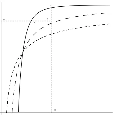
where the value of r > 0still remains to be chosen. Figure 2 plots the production equivalence surface deÞned through Þxing g(y, x) in a case where we have one good output and one bad output. The production equivalence surfaces are plotted forq(x) = 1.1 and various values ofr
(namelyr= 0.5,r= 1andr= 3). Note from (23) and Figure 2 that it is not possible to produce goods without bads; this is in line with the idea that bads are unavoidable by-products of the goods
production process and is implied by the deÞnition of null-jointness ine.g.F¨are, Grosskopf, Noh
and Weber (2002). This new output aggregator inspires the following deÞnitions.
Technical efÞciency,τT, is deÞned through
g
y1
τT
, . . . ,yp1 τT
, yp1+1, . . . , yp, x
=h(x)eε, (24)
which leads to
τT =e−γ
ηT
e−γq(x)η
T + 1−e−γq(x)
1/q(x)
, (25)
after deÞning
ηT =
p1
j=1α
q(x)
j y q(x)
j
p1
j=1α
q(x)
j y q(x)
j +
p
j=p1+1α
q(x)
j y
−rq(x)
j
. (26)
Note the similarity of (25) to the individual output-oriented efÞciency in (12), where we have
with equality only if ηT = 1 (inÞnite bads) or if γ = 0. The case of inÞnite bads2 can be interpreted as the situation where we focus entirely on producing goods and do not attempt to
reduce bad outputs, so that the technical efÞciency as measured by the goods only is equal to
the radial output-oriented efÞciency. In other cases, we sacriÞce some technical efÞciency as a
consequence of attempts to reduce pollution, due to the trade-off implicit in our aggregator. If we
focus on the caser = 3in Figure 2, a production level at pointAwill imply a technical efÞciency equal to|O2A|/|O2B2|.
Similarly, we can deÞne environmental efÞciency,τE, through
g
y1, . . . , yp1, τEyp1+1, . . . , τEyp, x
=h(x)eε, (27)
which, withg(y, x)as in (23), leads to
τE =e−γ/r
ηE
e−γq(x)η
E + 1−e−γq(x)
rq1(x)
, (28)
where we have deÞnedηE = 1−ηT as the relative contribution of the bads in the aggregator. In this case, τE ≤ exp(−γ/r)with equality only if ηE = 1(no goods3) or ifγ = 0. A graphical illustration of environmental efÞciency is given in Figure 2, by realizing that an observation atA
withr = 3inducesτE =|O1B1|/|O1A|.
In the context of data envelopment analysis (DEA), Tyteca (1996) discusses a measure of
environmental performance that is in the same spirit as the inverse of our τE. Again in a DEA
framework, F¨are, Grosskopf and Zaim (1999) consider an environmental performance index,
which is the ratio of a quantity index based on a measure akin toτT and an index derived from
the measure in Tyteca (1996) mentioned above.
4
Discussion of Related Work
There is an extensive literature which considers efÞciency deÞnitions closely related to those
presented here (see, e.g., F¨are and Primont, 1995). Although the terminology and notation is
different from ours, the basic ideas are quite similar. A key concept in this literature is the output
distance function,D0(x, y), deÞned as:
2As pointed out by a Referee, the aggregator in (23) does formally allow for unbounded quantities of bad output
withÞnite inputs, which is clearly not a literal reßection of reality. However, for empirically relevant combinations of good and bads, we feel the properties of our aggregator function are quite reasonable, and we would not want to use the model for predictions far outside the range of the data.
3
D0(x, y) = inf
θ:y
θ
∈P(x),
whereθis a scalar andP(x)is an output correspondence. That is,P(x)deÞnes the set of outputs which can be produced byx. It can be seen that our equation (4), with the measurement error
removed, deÞnes an output distance function and θ is equivalent to our radial output-oriented
efÞciency measure, τRO, in (9). An input distance function can be deÞned analogously and
related to our radial input-oriented efÞciency.
Most of the work using distance functions has been implemented using non-econometric
methods (e.g.Malmquist productivity indices are calculated using DEA techniques by, among
many others, F¨are, Grosskopf and Kirkley, 2000). Researchers who adopt econometric
ap-proaches include Atkinson, Cornwell and Honerkamp (2003) who use a single-equation
Gen-eralized Method of Moments methodology and Coelli and Perelman (2002) who use a
single-equation corrected OLS methodology. However, for likelihood-based inference, such as our
Bayesian analysis, we do need more than such a univariate distance function as we are required
to specify a distribution inpdimensions.
The concept of the distance function has been extended in,e.g., Chambers, Chung and F¨are
(1996) to the directional distance function. The output-oriented directional distance function is
deÞned as:
− →
D0(x, y, d) = sup{λ:y+λd∈P(x)},
wheredis ap×1direction vector andλis a scalar. The relationship between the output distance function and output-oriented directional distance function is obtained by settingd=yand noting:
D0(x, y) =
1 +−→D0(x, y, y) −1
.
The directional distance function can be used to measure inefÞciency in terms of distances from
an observation to the frontier in any direction. Thus, the close relationship between τjO and
− →
D0(x, y, dj) with dj = (0, . . . ,0, yj,0, . . . ,0)′ is clear. Our efÞciency shares also represent
another direction in which distance to the frontier can be measured. Directional distance
func-tions have typically been estimated using DEA techniques (see, e.g., Ball, F¨are, Grosskopf and
Nehring, 2001) and input-oriented directional distance functions can be deÞned which are closely
related to our individual input-oriented efÞciency measures. In the context of goods and bad
out-puts, F¨areet al.(2002) impose null-jointness and weak disposability of (good and bad) outputs
5
Applications
In this section, we investigate the properties of the various efÞciency measures in the context of
two substantive applications which have received attention in the applied literature. It is worth
noting that in both applicationsq tends not to be far from one for mostÞrms. This may help the
reader is assessing some of the properties of the expressions in Section 3. Reported results on
the banking data are based on a Monte Carlo run of 25,000 retained draws after discarding the
Þrst 5000, whereas results for the agricultural data correspond to a run of 60,000 and a burn-in of 10,000 draws.
5.1
Ef
Þ
ciency of the US Banking Industry
Berger and Humphrey (1997) provide an extensive survey of the literature on the efÞciency of
Þnancial institutions. We use a data set which has been used by several others to investigate this important issue (see Berger, 1993, Adams et al., 1999, and FKS). This banking data set
contains observations on N = 798 limited branching banks in the United States for T = 10
years (1980-89). The theory of bank behavior suggests that it is reasonable to treat loans as
an output in a production process where deposits and traditional factors (e.g.labor, capital) are
inputs. Accordingly, the data set contains p = 3 outputs (real estate loans; commercial and industrial loans; installment loans) and m = 5 inputs (average number of employees; physical capital; purchased funds; demand deposits; retail, time and savings deposits). A Cobb-Douglas
form is assumed for the production frontier. We assume thatγhas an individual effects structure
and, hence,D=IN ⊗ιT (see the discussion following (4)).
FKS carries out a Bayesian analysis of this data set. The model used in FKS contains
explana-tory variables in the efÞciency distribution, and imposes separability. With these exceptions, the
present model (described in Section 2 and the Appendix) is identical to that in FKS and results
are quite similar. We focus mainly on the differences with FKS and on efÞciency measurement.
Relative to FKS, we have extended our model to allow for nonseparability through (2) and, thus,
it is worthwhile to present results for ψ.4 Table 1 presents the medians of the posterior
distri-butions as point estimates and 95% Bayesian credible intervals5 for the m+ 1 elements ofψ.
Sinceψ1, . . . , ψ5 have most of the posterior mass quite close to zero, there is no immediate
ev-idence of a departure from separability of the transformation function (corresponding toψl = 0
4To aid in interpretation, note that the explanatory variables used forqin (2) have been standardized to take
values in[0,1].
forl = 1, . . . ,5). This is in line with the Bayes factor which mildly favors the separable model over the nonseparable one: the Bayes factor is estimated to be40.4in favor of the nonseparable model. This is based on the marginal likelihood values for each model, which are estimated using
the modiÞed harmonic mean estimatorp4 of Newton and Raftery (1994). Thus, for this data set,
there is no real evidence of nonseparability of the transformation function. However, we shall
present the results of the more general nonseparable model in the sequel (which are quite close
to those with the separable model). In addition, Table 1 tells us that the posterior forψ0is located
[image:16.595.200.411.257.393.2]very near to zero, indicating values ofq(x)≈1. Thus, in this application, we are near the limiting case of a linear production equivalence surface (see Figure 1a forq(x) = 1).
Table 1: Posterior Properties ofψ
95% Credible Interval
Median Lower Upper
ψ0 4.0×10⁻⁵ 1.0×10⁻⁷ 1.9×10⁻⁴
ψ1 2.9×10⁻³ 9.6×10⁻⁵ 1.5×10⁻²
ψ2 3.8×10⁻³ 1.4×10⁻⁴ 2.0×10⁻²
ψ3 7.3×10⁻³ 3.0×10⁻⁴ 3.8×10⁻²
ψ4 8.0×10⁻⁵ 5.9×10⁻⁶ 4.2×10⁻⁴
ψ5 1.5×10⁻⁴ 1.1×10⁻⁵ 3.4×10⁻⁴
We next investigate whether the use of various deÞnitions of efÞciency allows us to uncover
potentially interesting aspects of the data that would remain hidden if we focussed only on, say,
τRO. We begin with a simple analysis based only on point estimates of efÞciency. Note that strong
assumptions are necessary to derive classical conÞdence intervals for Þrm-speciÞc efÞciencies
(see Horrace and Schmidt, 1996) and common computer packages (e.g.LIMDEP) do not produce
conÞdence intervals. It is perhaps for these reasons, that applied work often merely presents point
estimates of efÞciencies (e.g., among many others, Barla and Perelman, 1989). We use posterior
means as point estimates.
Given the individual effects structure of γ, τRO will also have an individual effects
struc-ture. However,τjO andτjS will not (j = 1, . . . , p). Accordingly, for each of our 2p+ 1 = 7 output-oriented efÞciency deÞnitions, we have aT N-vector which contains the posterior means
of efÞciency for each bank in each time period. Table 2 presents the correlation matrix between
these seven vectors. This simple measure of linear interdependence is computed as the
correla-tion coefÞcient between pairs of observations, where pairs share the same(i, t) index. Table 3 presents the Spearman rank correlation matrix computed along the same lines.
ConsiderÞrst radial output-oriented efÞciency. All of the other efÞciency measures are
Table 2: Correlation Between Posterior Means of EfÞciency Measures
τRO τ1O τ2O τ3O τ1S τ2S τ3S 1.00
0.89 1.00
0.71 0.52 1.00 0.87 0.72 0.59 1.00 0.61 0.86 0.15 0.34 1.00
0.26 -0.02 0.75 0.04 -0.22 1.00
0.66 0.44 0.36 0.90 0.03 -0.10 1.00
Table 3: Rank Correlation Between Posterior Means of EfÞciency Measures
τRO τ1O τ2O τ3O τ1S τ2S τ3S 1.00
0.88 1.00 0.71 0.47 1.00 0.88 0.67 0.54 1.00 0.59 0.88 0.17 0.35 1.00
0.25 0.00 0.81 0.09 -0.18 1.00
0.65 0.41 0.33 0.92 0.10 -0.04 1.00
of these correlations are quite low (e.g. the correlation withτ2S). This provides preliminary
ev-idence that alternative efÞciency measures can provide a different perspective on the same data
set. Between the efÞciency shares weÞnd correlations near zero. This is not so surprising since
τjS =ηj1/q(x)τRO[see (14), whereq(x)takes values close to 1] and the correlation betweenηiand
ηj fori=j will be negative6. This implies a negative contribution to the correlation betweenτjS andτiS, which counteracts or even dominates the positive contribution through the common
fac-torτRO. Further, correlations betweenτiOandτjStend to be quite high fori=j but considerably lower fori=j.
As discussed above, the input-oriented efÞciency measures for the Cobb-Douglas production
frontier are always the same powers of radial output-oriented efÞciency in the separable case.
Given that the data favor the separable model, and the results presented here are very close to
those with that model, these powers will be quite an accurate approximation of the input-oriented
measures and, hence, the latter are not presented here.
Note that results using the Spearman rank and simple correlations are quite similar to one
an-other. We found this similarity in all of our results and, accordingly, do not discuss the Spearman
rank correlation in our subsequent empirical work.
6This is not counterintuitive, since theη
In order to further investigate the relationships between the different efÞciency measures, we
created scatterplots from the point estimates of efÞciency used to calculate the correlations in
Table 2. For the sake of brevity, we present only selected results. Figures 3, 4 and 5 plot the
point estimates ofτRO againstτjS forj = 1,2,3,respectively. As indicated in Subsection 3.3, we always haveτRO ≥τjSand, hence, the points in theÞgures all lie below the 45-degree line. It is clear that there are many observations which lead to substantially different efÞciency estimates
using the different efÞciency measures. The main conclusion we can draw from these Þgures
is that indeed τ2S behaves quite differently from the usual radial output-oriented efÞciency. In
particular, theÞrms that are closest to the frontier (withτRO > 0.8) seem to produce relatively less of the second output (commercial and industrial loans) and shift mostly to the third output
(installment loans). This conclusion was borne out by looking at scatterplots of posterior
esti-mates ofτROversusη. Thus, if we are particularly interested in how wellÞrms do in terms of the
second output (with respect to what they could produce if they gave up production of the other
outputs), the conclusions in terms of efÞciency levels and ranking ofÞrms will inevitably be very
different from those based onτRO.
If we conduct a similar comparison of radial and individual output-oriented efÞciencies, we
Þnd roughly similar results, although the differences are not that striking.
What should we make of our previous results? Clearly, we cannot say “It does not matter
which efÞciency deÞnition you choose, all will give essentially the same results”. However, in a
practical setting, the choice between different efÞciency measures is not likely to be completely
arbitrary. Researchers who are interested in departing from the standard radial-oriented output
measures, will typically have a reason to focus on a particular output (e.g.to measure the shortfall
of real estate loans from the maximum possible). Given the rather different interpretation of
in-dividual output-oriented efÞciency and efÞciency shares, it is not surprising that they would give
different results for some observations. Thus, what this really establishes is that the researcher
must make a choice between the various measures of output-oriented efÞciency. In addition, the
variety of efÞciency measures we present allows us to extract and highlight more information
from a given data set.
The numbers in the previous tables were obtained by Þrst calculating the posterior mean
for each Þrm and time period and then calculating correlations. This, of course, ignores the
estimation uncertainty inherent in any efÞciency analysis. A simple way to shed light on this is to
treat the correlations between efÞciency measures as random variables and plot their posteriors.
its posterior density function. This is done in Figures 6-8 for selected efÞciency measures. For
the sake of brevity, we do not plot the posteriors for all 2p2 +p correlations. Rather Figures
6 and 7 plot the posteriors for the correlations between τRO and each of τjO and τjS for j =
1, . . . , p. Figure 8 plots the posterior of the correlation between the individual output efÞciency
and efÞciency share measures for the same output (i.e. the correlation between τjO and τjS).
TheseÞgures do nothing to undermine our previousÞndings. That is, the correlations between
the efÞciency measures are fairly precisely estimated. Thus, our previous results based on point
estimates point in the same direction as those which properly address the issue of estimation
uncertainty.
Another way to consider the differences in efÞciency measures is to monitor whether Þrms
can make large jumps in the efÞciency ranking if we use a different measure. In order to do this,
we take the estimates of τRO for eachÞrm, rank them, and select the Þrms ranked at the Þrst,
second and third quartiles. We then calculate the posterior probability that the relative ranking of
each pair ofÞrms is maintained, using each of the efÞciency measures.
Table 4 contains the results. If we begin by examining the column labelled τRO, we can
see that rankings based on point estimates do give a crude but reliable picture ofÞrm-speciÞc
banking efÞciency. That is, the Þrm ranked as being at the 3rd quartile is almost always more
efÞcient than the median and 1st quartileÞrms. ThisÞnding indicates that if a researcher decides
on one particular efÞciency deÞnition (e.g.τRO), then the large spread of efÞciencies (evidenced
in Figures 3-5) does not prevent at least an approximate classiÞcation of observedÞrms in terms
of their mean efÞciency levels.
Table 4: Probability that Firm A is More EfÞcient than Firm B
Firm A/Firm B τRO τ1O τ2O τ3O τ1S τ2S τ3S 3rd Quart./Median 0.98 0.94 0.25 1.00 0.68 0.00 1.00 3rd Quart./1st Quart. 1.00 1.00 1.00 1.00 0.29 0.04 1.00 Median/1st Quart. 1.00 0.90 1.00 1.00 0.18 1.00 1.00
Three of the columns of Table 4 exhibit a similar pattern. In particular, usingτ1O,τ3Oorτ3S
as efÞciency measures would lead to a similar differentiation between these three Þrms as the
one based onτRO. However, the other efÞciency deÞnitions indicate somewhat different rankings
of the threeÞrms. Tables 5 and 6 present posterior means and standard deviations, respectively,
for the efÞciencies of the three Þrms using all of the deÞnitions. We know that the absolute
magnitudes of the various efÞciencies are subject to the inequalities in (15). An examination
of these tables immediately puts the results in Table 4 in context. Posterior standard deviations
However, the three Þrms selected as being at theÞrst, second and third quartiles usingτRO are
ranked quite differently using some of the other efÞciency deÞnitions. In particular, the Þrm
ranked as being quite efÞcient byτRO (i.e.the third quartile), is quite inefÞcient according toτ2S
and is below the median according toτ2O. In addition, all threeÞrms have roughly equal values
forτ1S. Thus, the results of Tables 5 and 6 highlight the need for a careful choice of the efÞciency
measure used, depending on the question one wants to address.
Table 5: Posterior Means of EfÞciencies for Three Firms
Ranking acc. toτRO τRO τ1O τ2O τ3O τ1S τ2S τ3S
3rd Quartile 0.73 0.35 0.44 0.57 0.15 0.21 0.37
Median 0.63 0.28 0.47 0.31 0.14 0.33 0.16
1st Quartile 0.51 0.24 0.32 0.19 0.15 0.24 0.12
Table 6: Posterior Standard Deviations of EfÞciencies for Three Firms
Ranking acc. toτRO τRO τ1O τ2O τ3O τ1S τ2S τ3S
3rd Quartile 0.04 0.04 0.04 0.04 0.01 0.01 0.02
Median 0.04 0.03 0.04 0.03 0.01 0.02 0.01
1st Quartile 0.02 0.02 0.02 0.01 0.01 0.01 0.01
Incidentally, the posterior mean value forτRO corresponding to the medianÞrm accords well
with the estimated average relative efÞciencies computed for these data on the basis of
non-parametric methods in Adamset al.(1999).
Researchers may worry about presenting Þrm-speciÞc efÞciency estimates or rankings on
the grounds that posterior standard deviations might be large and, hence, point estimates might
be misleading. Alternatively, they may worry about the choice of efÞciency deÞnition. Our
Þndings above indicate that it is the latter issue that is the more serious one. Posterior standard deviations, at least for the present application, are not so large as to preclude at least a rough
categorization ofÞrms in terms of their efÞciency. However, alternative efÞciency deÞnitions can
give very different results. Thus, we should carefully choose the efÞciency measure that is the
most appropriate one to answer the question of relevance to us in a particular empirical situation.
5.2
An Application to Dutch Dairy Farms
Stochastic frontier methods have been extensively used in the Þeld of agricultural economics.
As an example in this area, we use a data set compiled by the Agricultural Economics Research
Institute in the Hague from highly specialized dairy farms that were in the Dutch Farm
describe the data in detail. The panel is unbalanced and we have 1,545 observations onN = 613
dairy farms in the Netherlands for some or all of 1991-94. The dairy farms produce three outputs
(p= 3), one of which is bad (p1 = 2) using three inputs (m = 3):
• Good Outputs: Milk (millions of kg) and Non-milk (millions of 1991 Guilders).
• Bad Output: Nitrogen surplus (thousands of kg).
• Inputs: Family labor (thousands of hours), Capital (millions of 1991 Guilders) and Variable input (thousands of 1991 Guilders).
Variable input includes inter alia hired labor, concentrates, roughage and fertilizer.
Non-milk output contains meat, livestock and roughage sold. The deÞnition of capital includes land,
buildings, equipment and livestock.
Fern´andez et al. (2002) analyze the same data, using two separate Cobb-Douglas frontiers
(one for the goods and one for the bad). Here, we assume a translog form for the single production
frontier, as in Reinhard et al. (1999). Hence, using the notation following equation (4), and
denoting thelth element ofx(i,t)byx(i,t,l), we havek = 10and:
v(x(i,t)) = (1,ln(x(i,t,1)), . . . ,ln(x(i,t,3)),ln2(x(i,t,1)),ln(x(i,t,1)) ln(x(i,t,2)),
. . . ,ln(x(i,t,2)) ln(x(i,t,3)),ln2(x(i,t,3)))′.
We experimented with different values forrin the aggregator function (23) and found the results
relatively insensitive to the actual choice ofrin the range 0.5 to 3. We shall present our results
forr = 3. Again, we assume an individual effects structure forγ.
As before, we focus mainly on the efÞciencies. As in the case of the banking data, the data
favor separability in the production frontier. Marginal likelihoods computed using the estimator
p4 of Newton and Raftery (1994) lead to a Bayes factor of63.2in favor of the separable model.
Thus, the evidence that the elasticity of transformation does not depend on the inputs used is
even stronger for the farm data than for the banking data. Separability also greatly facilitates the
calculation of input-oriented efÞciencies (see Subsection 3.4), which we want to examine in this
translog application. Therefore, we now only present results for the separable model.
Table 7 presents the correlations between the measures of efÞciency introduced in Section 3,
including the input-oriented measures and the technical and environmental efÞciencies of
Sub-section 3.5. Results using Spearman rank correlations are very similar.
All input-oriented measures are highly correlated among themselves, and also display a high
Table 7: Correlation Between Posterior Means of EfÞciency Measures
exp(−γ) τ1O τ2O τ1S τ2S τRI τ1I τ2I τ3I τT τE 1.00
0.98 1.00
0.56 0.44 1.00
0.91 0.97 0.23 1.00
0.05 -0.11 0.72 -0.34 1.00
0.98 0.97 0.52 0.91 0.04 1.00
0.76 0.75 0.65 0.70 -0.01 0.70 1.00
0.88 0.87 0.53 0.82 -0.02 0.85 0.81 1.00
0.88 0.85 0.66 0.76 0.10 0.83 0.87 0.90 1.00
1.00 0.98 0.56 0.92 0.06 0.98 0.75 0.87 0.87 1.00
-0.46 -0.50 -0.18 -0.50 -0.04 -0.61 -0.18 -0.39 -0.32 -0.51 1.00
For output 2-oriented measures this is not the case (especially for efÞciency shares). Clearly,
efÞciency measurement corresponding to output 2 (non-milk) is not very similar to the other
measures. Technical efÞciency [as deÞned in (25)] is highly positively correlated with all other
measures, except for those in the direction of output 2 andτE. Posterior mean environmental
efÞciency [see (28)] is clearly negatively correlated with the other efÞciency measures, and in
particular, has a correlation of−0.51with the technical efÞciency for the good outputs,τT. This result is in contrast with the small positive correlation found in Fern´andezet al. (2002). Note,
however, that in the latter paper environmental and technical efÞciency are modeled separately,
whereas here they reßect different ways of looking at the same distance with respect to the (single)
frontier.
The relationship between exp(−γ) 7 and the various input-oriented efÞciency measures is
further illustrated in Figures 9-12, where it is clear that the relationship bears some resemblance
to the powers ofexp(−γ)that result from the simpler Cobb-Douglas frontier [see (18) and (19)]. Table 8 is the counterpart of Table 4, where we have chosen three quartileÞrms according to
[image:22.595.55.553.611.691.2]exp(−γ), and consider the posterior probabilities that a higher rankedÞrm is more efÞcient than a lower ranked one.
Table 8: Probability that Firm A is More EfÞcient than Firm B
Firm A/Firm B exp(−γ) τ1O τ2O τ1S τ2S τRI τ1I τ2I τ3I τT τE
3rd Quart./Median 0.99 0.99 0.97 0.99 0.78 0.83 0.85 0.33 0.86 0.99 1.00
3rd Quart./1st Quart. 1.00 1.00 0.01 1.00 0.00 1.00 0.94 0.81 0.91 1.00 1.00
Median/1st Quart. 0.99 1.00 0.00 1.00 0.00 1.00 0.77 0.99 0.39 0.99 0.00
7Note that here we do not useτ
Table 8 paints the same broad picture as Table 7, in that the efÞciency measures are roughly
in accordance, except for output 2-oriented and environmental efÞciency. In order to get an idea
of typical regions for the various efÞciencies, Table 9 presents the averages and standard
devia-tions (computed over all observadevia-tions) of the posterior mean efÞciencies. Clearly, the inequality
[image:23.595.83.525.178.242.2]constraints mentioned in Section 3 can be recovered in the means.
Table 9: Posterior Means of EfÞciency Measures
exp(−γ) τ1O τ2O τ1S τ2S τRI τ1I τ2I τ3I τT τE
Average 0.68 0.65 0.18 0.60 0.07 0.63 0.11 0.41 0.29 0.67 0.15
St.Dev. 0.13 0.14 0.14 0.14 0.06 0.17 0.11 0.19 0.20 0.13 0.12
Note the large difference between the output-oriented efÞciency measures corresponding to
the two good outputs. Clearly, Þrms tend to be much more efÞcient in the direction of milk
production (output 1) than in that of non-milk production. Given that the primary goal of these
farms is milk production, their infrastructure will be mostly geared towards that aim, and this
difference is not too surprising. The average of the posterior mean efÞciencies in Table 9 would
correspond to a Þrm that is much closer to the horizontal (“milk”) axis than the vertical
(“non-milk”) axis in Figure 1b, and produces 65% (τ1O) of the milk output that it could produce, given
the current level of non-milk production. If it would also relinquish its non-milk production, it
is at 60% (τ1S) of its maximum milk output. However, if thisÞrm would consider giving up its
milk production, it could multiply its production of non-milk output more than tenfold (seeτ2S)!
Radial input-oriented efÞciency is in the same region as exp(−γ), and the input that seems least efÞciently used is the Þrst one, namely family labor (which presumably is often readily
available).
Of particular interest are also the technical and environmental efÞciencies, and from Table 9
we clearly see thatÞrms tend to do better in producing goods than in avoiding the production of
the bad (nitrogen surplus). A more insightful picture of technical and environmental efÞciencies
can be obtained by a predictive concept. The out-of-sample predictive efÞciency distributions
capture the inference on efÞciencies for an unobservedÞrm belonging to the industry. This is
obtained by integrating out the efÞciency distributions with the posterior. Given the deÞnition
ofτT andτE, we need to integrate the distribution of z (and thusγ) in (A.2) with the posterior
distribution ofφand the distribution ofη in (7) with the posterior ofs, as well as use the
poste-rior of ψ and αto deÞneq(x) in (2)8 and η in (6). Given posterior draws from (φ, s, ψ, α), we
8Hereq(x)is simply equal to(1 +ψ
0)as we are in the separable case. In general,q(x)does depend on inputs,
can thus construct draws for technical and environmental efÞciencies. This results in the
predic-tive efÞciencies graphed in Figures 13 and 14, along with the efÞciencies of the three quartile
observations chosen for Table 8. The latter illustrate that knowledge of the speciÞc Þrm-year
greatly reduces the uncertainty in efÞciency inference. This, once again, illustrates the possibility
of rankingÞrms according to efÞciencies in a meaningful way (although we should not attach
too much importance to small differences in rank). Predictive means and standard deviations (in
parentheses) ofτT andτE are0.701 (0.220)and0.244 (0.221), respectively. If we compare these predictive distributions with those presented in Fern´andezet al.(2002), we obtain here a slightly
higher technical efÞciency and a somewhat lower environmental efÞciency. The overall picture,
though, is similar, in that uncertainty about efÞciencies of unobserved Þrms is substantial and
environmental efÞciency tends to be considerably lower than technical efÞciency.
It is worth noting that this paper focuses on multiple-output production. If there is only a
single output, then all of our output-oriented measures are equivalent to one another. However, the
input-oriented measures are still different from one another. Hence, the issues andÞndings in this
application for the input-oriented measures are of relevance for the single-output case. Atkinson
and Cornwell (1994) provide a detailed discussion of output and input-oriented measures in the
single equation case.
6
Conclusions
In this paper, we have derived and discussed various ways of deÞning efÞciency with
multiple-output production, where we allow for nonseparability of multiple-outputs and inputs. In addition to
standard radial measures we discuss the properties of individual output-oriented measures. We
also considered analogous input-oriented efÞciency deÞnitions. Furthermore, we developed an
efÞciency measure which incorporates the losses due to jointness in production, and which we
refer to as “efÞciency shares”. Finally, we deÞned technical and environmental efÞciencies in
cases where some of the outputs are undesirable by-products. With so many alternative ways of
deÞning efÞciency, the question arises as to which deÞnition to adopt. This paper provides two
types of responses to this. Firstly, in many applications the choice of efÞciency measure is not
arbitrary. Each measure has a particular interpretation and it is crucial to use the measure that
corresponds to the particular empirical question being raised. For instance, the researcher may
have reason to focus on one particular output or input and, hence, useτjO orτjI. Alternatively,
the researcher may be interested in what would happen if only one output were produced, in
than one efÞciency measure allows us to obtain a much clearer picture of the data, through the
decomposition of the distance to the frontier (γ) in various complementary and often insightful
ways.
We have illustrated the issues above in the context of two substantive applications, where we
also demonstrated that the types of things a policymaker might want to report (e.g.an efÞciency
ranking or the identiÞcation of someÞrms as laggards or exemplars) do seem to make practical
sense, once we have agreed on a particular choice of efÞciency deÞnition.
Nevertheless, our results do highlight that caution should be taken when carrying out an
ef-Þciency analysis. We would recommend that practitioners report posterior standard deviations (or conÞdence intervals) of all Þrm-speciÞc efÞciency estimates. Furthermore, if theoretical
considerations do not provide clear guidance as to which efÞciency deÞnition should be used,
researchers should present results for several different choices.
Acknowledgements
We acknowledge funding by the UK Economic and Social Research Council under grant number
R34515. We are grateful to two referees and a guest co-editor for helpful and thought-provoking
comments that have led to improvements in the paper. We would also like to thank Robert Adams,
Allen Berger and Robin Sickles for providing the banking data used in this paper, and Stijn
Reinhard and the Dutch Agricultural Economics Research Institute (LEI-DLO) for providing the
agricultural data.
Appendix: Bayesian Analysis
The Prior Distribution
In order to conduct Bayesian inference, we need to complement the likelihood function (as
de-scribed in Section 2) with a prior distribution on the parameters(β, z, σ, α, q, s). We shall choose a proper prior distribution with the following structure
p(β, z, σ, α, q, s) =p(β)p(z)p(σ)p(α)p(q)p(s). (A.1)
It is worthwhile brießy noting that use of improper priors in stochastic frontier models can
cause problems (i.e.inability to calculate meaningful Bayes factors or even the lack of existence
of the posterior itself, see Fern´andezet al., 1997, for details). In this paper, we choose values for
Prior forz:
The distribution ofzdetermines the distribution of the inefÞciency vectorγ =Dz. Since we are assuming an individual effects structure for the inefÞciencies, z ∈ ℜN
+. We will consider a
hierarchical structure which adds an extra parameterφ ∈ ℜ+. Givenφ, we take the following
product of Exponential distributions for the elements ofz:
p(z|φ) =
N
l=1
fG(zl|1, φ) , (A.2)
wherefG(zl|a, b)denotes the p.d.f. of a Gamma distribution with meana/b and variancea/b2. The prior onφis taken to be
p(φ) =fG(φ|e0, g0), (A.3)
with positive prior hyperparameterse0 andg0. We choosee0 = 1andg0 = −log(0.80), values
which imply a relativelyßat prior on the individual efÞciencies with prior median efÞciency set
at 0.80, as discussed in van den Broecket al.(1994).
Prior forβ:
The prior assumed on the frontier parameters has p.d.f.
p(β)∝fNk(β|b0, H0−1)IB(β),
i.e.ak-dimensional Normal distribution with meanb0 and covariance matrixH0−1, truncated to
the regularity regionB. In ourÞrst application, we assume a Cobb-Douglas form for the frontier. Hence, IB(β) corresponds to simply restricting the elements of β (except the intercept) to be
non-negative. In our second application, we use a translog frontier and we impose only local
regularity (i.e.we impose regularity at each data point). Hence,IB(β)corresponds to the region
where input elasticities are non-negative at every data point [see the discussion after equation
(22)]. We setb0 = 0kandH0 = 10−4×Ik. Thek−1last elements ofβare likely to be smaller than 1. Due to the logarithmic transformation, the intercept will also certainly be much less than
one prior standard deviation away from the mean. Hence, our prior is quite noninformative.
Prior forσ:
We deÞne the prior distribution on the scaleσ, through a Gamma distribution on the precision
h=σ−2:
p(h) =fG(h|n0/2, a0/2). (A.5)
In our applications, we setn0/2 = 1(which leads to an Exponential prior forh) anda0/2 = 10−6.