SrTiO3 (001) (2x1) reconstructions : first-principles calculations of surface energy and atomic structure compared with scanning tunnelling microscopy images

SrTiO

„

001

…„

2

Ã

1

…

reconstructions:

First-principles calculations of surface energy and atomic

structure compared with scanning tunneling microscopy images

Karen Johnston,*Martin R. Castell,†_{Anthony T. Paxton, and Michael W. Finnis}

Atomistic Simulation Group, Department of Pure and Applied Physics, Queen’s University Belfast, Belfast BT7 1NN, Northern Ireland, United Kingdom

(Received 23 February 2004; published 26 August 2004)

共1⫻1兲and共2⫻1兲reconstructions of the(001) SrTiO3surface were studied using the first-principles

full-potential linear muffin-tin orbital method. Surface energies were calculated as a function of TiO2 chemical

potential, oxygen partial pressure and temperature. The 共1⫻1兲 unreconstructed surfaces were found to be energetically stable for many of the conditions considered. Under conditions of very low oxygen partial pressure the共2⫻1兲Ti₂O₃reconstruction[Martin R. Castell, Surf. Sci. 505, 1(2002)]is stable. The question as to why STM images of the 共1⫻1兲surfaces have not been obtained was addressed by calculating charge densities for each surface. These suggest that the共2⫻1兲 reconstructions would be easier to image than the

共1⫻1兲surfaces. The possibility that the presence of oxygen vacancies would destabilise the共1⫻1兲surfaces was also investigated. If the共1⫻1兲 surfaces are unstable then there exists the further possibility that the共2

⫻1兲DL-TiO₂reconstruction[Natasha Erdman et al. Nature(London) 419, 55(2002)]is stable in a TiO₂-rich environment and for pO2⬎10

−18_atm.

DOI: 10.1103/PhysRevB.70.085415 PACS number(s): 68.35.Bs, 68.35.Md, 68.37.Ef, 68.47.Gh

I. INTRODUCTION

General interest in the properties of metal oxide crystal surfaces has emerged from such diverse fields as catalysis, corrosion, microelectronics, and gas sensing.1 Surface stud-ies on SrTiO3 crystals in particular are relevant to

applica-tions involving thin film growth where they are commonly used as a substrate. Exploitation of the dielectric properties has stimulated research into the creation of SrTiO₃thin films. Knowledge of the atomic scale structure of the surfaces is central to developing a fundamental understanding of SrTiO3

properties especially those related to very thin film growth where the nature of the interface is significant.

The unreconstructed (001) surface of perovskite SrTiO₃ has two possible charge neutral terminations. Due to their stoichiometry the terminations are referred to as the TiO2

and SrO surfaces. Numerous reports of surface studies on the 共1⫻1兲terminations exist, and indeed our first principles cal-culations in this paper show that they have low energy and are expected to be very stable. The traditional picture of the unreconstructed(001) surface is of 共1⫻1兲 regions of TiO2

and SrO terminations separated by half unit cell height steps as shown in Fig. 1(a). Surprisingly there are no atomic reso-lution scanning tunneling microscopy(STM)images of this type of surface termination. It is possible to create clean flat surfaces of SrTiO3 (001) with large terraces but when

im-aged in the ultra high vacuum (UHV) environment of the STM they are always reconstructed in some form and only have one type of termination with full unit cell height steps. STM images of the共2⫻1兲, c共4⫻4兲, c共2⫻4兲, c共6⫻2兲, and 共6⫻2兲 reconstructions have been reported in the literature.2–5 _{UHV transmission electron microscopy(TEM)}

analysis of the共2⫻1兲and c共2⫻4兲reconstructions have also been published.6,7_{In this paper we will focus on the possible}

origin and structure of the 共2⫻1兲 surface and discuss the

possibility that there may be more than one reconstruction with a共2⫻1兲 surface unit cell.

The three candidate structures that currently exist for the 共2⫻1兲 reconstruction are shown in Figs. 1(b)–1(d). In Fig. 1(b)alternate rows of oxygen have been removed from the TiO₂ terminated 共1⫻1兲 surface to create a 共2⫻1兲 surface with a reduced surface stoichiometry of Ti2O3 and it will

therefore be referred to in this paper as the 共2⫻1兲 Ti2O3

surface.4 Figure 1(c) shows a proposed structure with re-duced surface coverage of Ti but maintaining the TiO2

sto-ichiometry and will be called the 共2⫻1兲 TiO2 surface.4 A

further possibility proposed by Erdman et al.6 _{is shown in}

Fig. 1(d). It is an unusual structure in that the surface has a double layer TiO2termination and it will be referred to as the

共2⫻1兲DL-TiO2surface. Reconstructions that are SrO

termi-nated are not considered here as most experimental data in-dicate a Ti rich termination.

Kubo and Nozoye8 have recently made the interesting suggestion that reconstructions observed can be explained as arising from patterns of Sr adatoms on a TiO₂ terminated 共1⫻1兲surface, although this has not been backed up by free energy calculations.

Given the stability of the 共1⫻1兲 surfaces, why then are there no atomic resolution STM images? There are two likely explanations. The共1⫻1兲 terminations may simply be too electronically flat to allow atomic resolution STM imag-ing which is the reason postulated for the difficulty in obtain-ing atomic resolution images of CoO(001)共1⫻1兲.9

Alterna-tively, the SrTiO3 共1⫻1兲 terminations might simply not be

stable in a realistic UHV experiment. When preparing a crys-tal to examine its surface atomic layer it must be clean and ordered. To produce a surface free of adsorbates it is neces-sary to anneal it in UHV conditions which in turn will en-courage surface oxygen defects to be created. We show in this paper that under certain conditions a 共2⫻2兲 unit cell

with a missing oxygen atom has a higher surface energy than the共2⫻1兲reconstructions. It is therefore quite possible that a perfect共1⫻1兲termination is stable in UHV conditions, but as soon as an oxygen atom is lost into the vacuum this results in local共2⫻1兲ordering which in turn causes more oxygen loss and hence more共2⫻1兲 ordering. A clean surface with large 共1⫻1兲 terraces suitable for UHV STM imaging will therefore rapidly reconstruct to a共2⫻1兲surface.

The paper is organized as follows: Sec. II describes the method of total energy calculations. Section III describes in detail the theory used to treat nonstoichiometric surfaces and includes a derivation of the temperature and pressure depen-dence of the chemical potential of oxygen. The results of surface relaxations, surface energies and charge densities are presented in Sec. IV and V as well as a discussion of their implications. The final section summarizes the main conclu-sions of this work.

II. METHOD OF TOTAL ENERGY CALCULATIONS

We have used the full-potential linear muffin-tin orbitals (FP-LMTO) method written by Methfessel and van

Schilfgaarde.10,11_{This method implements density functional}

theory within the local density approximation (LDA). We have not included gradient corrections to the LDA exchange and correlation functional. This would not add to the com-putation time, but we have have found in earlier work on stoichiometric and reduced surfaces of TiO2that these do not

affect surface energies or structures although they do tend to overestimate the magnetic moment if there are unpaired spins.12_{The basis functions are envelopes of “smooth”}

Han-kel functions(which are convolutions of solid Hankel func-tions and Gaussians)augmented within atomic spheres with numerical solutions of the radial Schrödinger equation ( in-cluding scalar relativistic corrections).

For SrTiO₃ we have used a basis consisting of Sr 5s , 5p , 4d, Ti 4s , 4p , 3d, and O 2s , 2p , 3d orbitals. The Sr 4p and Ti 3p orbitals were included in the basis as “local orbitals”.13 _{The atomic sphere radii were 2.4 a.u. for Sr,}

2.12 a.u. for Ti, and 1.45 a.u. for O. The Sr 4s and Ti 3s core states were treated with the frozen overlapped core approxi-mation.

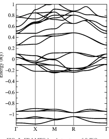
For bulk calculations a Brillouin zone mesh of 4⫻4⫻4 and a Fourier transform mesh of 32⫻32⫻32 were used. The calculated electronic bandstructure is shown in Fig. 2. The band gap is approximately 0.13 Ry共1.79 eV兲 which com-pares well to the previous calculations in Ref. 14 who ob-tained a band gap of⬇2 eV. The equilibrium lattice constant of SrTiO3was found to be a0= 3.85 å and the bulk modulus

was K = 200 GPa. The elastic constants were c

⬘

are a0= 3.905 Å,15 K = 184 GPa,15 c

⬘

= 128 GPa.16 _{The error between the theoretical values and}

experimental values are typical of the LDA which tends to overbind the system.

All our calculations of the various surface structures were performed using the theoretical lattice constant. The Bril-louin zone mesh and the Fourier transform mesh were scaled to correspond with those used for the bulk unit cell.

FIG. 1. (a) 共1⫻1兲 unreconstructed TiO2and SrO surfaces.(b)

共2⫻1兲 Ti2O3 reconstruction. (c) 共2⫻1兲 TiO2 reconstruction. (d)

共2⫻1兲 DL-TiO2 reconstruction. Ti atoms are darkest and O are

lightest.

Surfaces are represented in our calculations by periodi-cally repeating slabs separated by vacuum having a thickness in the range 1 – 3 a0.

III. THEORY OF NONSTOICHIOMETRIC SURFACES

The theory necessary to compare the free energy of sur-faces with different stoichiometries has been described in Refs. 17–19. In this section we summarize the general prin-ciples and include a fuller description than before of how to account for the oxygen partial pressure.

Since we are dealing with a two phase system made up of three components, the phase rule tells us that we have three degrees of freedom. It is convenient to choose these to be the chemical potential of TiO2, the partial pressure of oxygen

(equivalent to its chemical potential), and the temperature:

␮TiO₂, pO₂, T. With these three parameters specified, the

sur-face excess free energy is calculated for a particular structure and stoichiometry as

␴共␮TiO₂, pO₂,T兲=

1 2As

冉

Gs−

兺

i

␮iNi

冊

where Gs is the Gibbs free energy of the slab, Ni is the

number of each component i within the slab, and␮i is the chemical potential of component i per formula unit. Asis the

area of one of the surfaces of the slab and the factor of 1₂ accounts for the fact that there are two surfaces per slab. The idea is that the predicted surface structure would be the one that minimizes(1). Although the theory implicitly takes into account the temperature and pressure of the oxygen in the vapour phase, the calculations for the solid will be done at a temperature of absolute zero. This approach also leaves out in practice any consideration of either configurational en-tropy or vibrational enen-tropy associated with the surface structure. The former is not significant for ordered surfaces such as the ones we are dealing with, while the latter error would certainly be significant in deciding between closely competing surface structures.

The surface free energy can also be expressed in terms of the excesses⌫_iof the components. The surface excess⌫_iof component i with respect to component A is

⌫i=

1

As

冉

N_ibulk

N_Abulk

冊

We choose component A to be SrO and introduce the surface excesses of TiO2 and O, in terms of which the surface free

energy is now

␴= 1 2As

共Gs− NSrOgSrTiO₃兲−␮TiO₂⌫TiO₂− 1

2␮O2⌫O, 共3兲

where gSrTiO₃is the Gibbs free energy of a bulk formula unit

of SrTiO3. The surface excesses⌫TiO₂ and⌫Ofor each

sur-face are listed in Table I.

The relative stability of the different surface structures depends on the chemical potentials which are discussed in the following subsections.

A. Chemical potential of TiO2

We cannot calculate ␮TiO

2 for the particular conditions under which the observed surface structures were created, but we can put bounds on it by the standard method applied in Ref. 20 as we now describe. For this we introduce ⌬G_f,SrTiO

3

0

, defined as the Gibbs free energy of formation of one formula unit of bulk SrTiO3 with respect to SrO and

TiO2, so that

⌬G_f,SrTiO

3

0 _{= g}

SrTiO₃

0 _{− g}

SrO 0

− g_TiO 2

0 _{, 共4兲}

where ⌬G_f,SrTiO

3

0 _{⬍0. g}

SrTiO₃

0 _{, g}

SrO 0 _{and g}

TiO₂

0 _{are the Gibbs}

free energies of the bulk crystal per formula unit in their standard states and in our work they are approximated by their 0 K total energy. SrO was calculated in the rocksalt structure, TiO2in the rutile structure, and SrTiO3was

calcu-lated in the cubic perovskite structure. The difference in en-ergy between the ideal cubic perovskite structure and the relaxed low temperature structure was considered to be in-significant. The formation energy was calculated to be ⌬G_f,SrTiO

3

0

= −0.1094 Ry.

The equilibrium of the slab requires that

gSrTiO₃=␮SrO+␮TiO₂. 共5兲

Neglecting the temperature dependence and stoichiometry variation of the free energy of bulk SrTiO3, then gSrTiO₃

= g_SrTiO 3

0

and

␮SrO+␮TiO

2= gSrTiO3

0 _{, 共6兲}

which confirms explicitly that only one of these chemical potentials is an independent degree of freedom. Neither

␮TiO₂ nor␮SrO can be predicted in the system under study, because the equilibrium conditions prevailing at the surface are not known. However it is known that

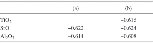
TABLE II. Standard oxygen chemical potential␮_O

2

0 _{in Ry, (a)}

from Gibbs energies, and(b)from enthalpies.

(a) (b)

TiO2 −0.616

SrO −0.622 −0.624

Al2O3 −0.614 −0.608

TABLE I. Surface excesses of subunits TiO2and O with respect

to SrO for different surface terminations. A_s共1⫻1兲is the area of one of the surfaces of a共1⫻1兲terminated slab.

Surface A_s共1⫻1兲⌫_TiO

2 As

共1⫻1兲 ⌫O

共1⫻1兲 TiO2 1

Ⲑ

共1⫻1兲 SrO − 1

Ⲑ

共2⫻1兲 TiO2 0 0

共2⫻1兲 Ti2O3 1

Ⲑ

Ⲑ

␮TiO₂艋g_TiO

2

0

, 共7a兲

␮SrO艋g_SrO0 , 共7b兲 because otherwise TiO₂or SrO, respectively, would precipi-tate out of the slab. Combining Eqs. (6) and (4) and the inequalities(7a)and(7b)gives

g_TiO

2

0

+⌬G_f,SrTiO

3

0 _艋␮TiO

2艋gTiO2

0

. 共8兲

Therefore at␮TiO 2= gTiO2

0

the system is in equilibrium with TiO₂ and SrTiO₃and at ␮TiO

2= gTiO2

0 _+⌬G f,SrTiO₃

0 _{the system}

is in equilibrium with SrO and SrTiO3.

B. Chemical potential of O2

We seek an expression for␮O

2共pO2, T兲, since pO2 and T are the parameters that can be related most directly to experi-mental conditions. At temperatures above 300 K and pres-sures at or below atmospheric, we can use the ideal gas equa-tions to high accuracy if we also make use of experimental thermochemical data to establish the correct reference points for enthalpy and entropy, thereby avoiding errors inherent in first-principles calculations of the free energy at low tem-peratures. The procedure works as follows. We take as a reference point the chemical potential of oxygen at standard pressure and temperature,␮O

2共p

0_{, T}0_{兲, henceforth written as} ␮O

2

0 _{, and obtain␮O}

2共pO2, T兲by integrating along the pressure and temperature axes in turn. The value of ␮O

2共p

0_{, T}0_{兲 is}

obtainable from compilations of thermochemical data, but these work with an energy zero such that oxygen has zero enthalpy in its standard state, whereas our zero of energy is established by the method of first-principles total energy cal-culation. We nevertheless make use of thermochemical data as much as possible, since they include entropic and quan-tum statistical terms that we can avoid calculating directly.

1. Calculation of␮_O

2

0

The chemical potential is defined in terms of the enthalpy and entropy per molecule in the standard state by

␮O₂共p_O

2

0 _,T0_{兲 ⬅␮O}

2

0 _{= h} O₂ 0 _{− T}0_s

O₂

0 _{. 共9兲}

Now the standard enthalpies per molecule of the components in an oxide(for this purpose we first take alumina, but any oxide will do)are related by

h_Al

2O3

0 _{= 2h}

Al 0 ₊3

2hO2

0 ₊ 1

N_A⌬Hf,Al2O3

0 _{, 共10兲}

where⌬H_f,Al

2O3

0 _{is the standard heat of formation per mole}

and NA is Avogadro’s number. We obtain the value of

⌬H_f,Al

2O3

0 _{from the NIST tables of thermochemical data}21

since its value does not depend on the choice of energy zero. The values of h_Al

2O3

0 _{and h} Al

0 _{are estimated as the total}

ener-gies per molecule in these crystalline solids, which we have calculated at 0 K. Hence Eq.(10)provides us with the value of h_O

2

0

. The standard entropy of oxygen s_O 2

0

is also obtained directly from tables of thermodynamic data, and combining

it in (9) with our estimate of h_O 2

0

we obtain our required value for ␮O

2

0 _{. An alternative strategy is to take our}

calcu-lated energies of the solids to be estimates of Gibbs free energies rather than enthalpies. A comparison of the values of ␮O

2

0

obtained from three different oxides, and with both strategies, is shown in Table II. In theory of course the results should be independent of the oxide used, but since we have consistently omitted the thermal energy of the oxides in our calculations, there is some variation of our calculated ␮O

2

0

with oxide and according to whether we assume we are es-timating the Gibbs energies or the enthalpies. For subsequent calculations we take the value ␮O

2

0

= −616 mRy. The calcu-lated␮O

2

0

span a range of 16 mRy⬇0.2 eV= 21 kJ mol−1, so a reasonable estimate of the error in our calculated ␮O

2

0

would be 8 mRy, or 0.1 eV.

2. Integration from␮_O

2

0

to␮O2„pO2, T…

First, to get to any required pressure pO₂ from the

refer-ence pressure p0 _{共1 atm兲at some constant temperature T we}

can apply the standard thermodynamic relation to a perfect gas,

冏

⳵p

冏

=kT

p , 共11兲

where k is Boltzmann’s constant, which gives the well-known formula

TABLE III. Coefficients for enthalpy and entropy expressions in Eqs.(16)and(17)for O₂.a

A 29.659 ⫻10−3 kJ mol−1K−1

B 6.137261 ⫻10−6 _{kJ mol}−1_K−2 C −1.186521 ⫻10−9 kJ mol−1K−3

D 0.095780 ⫻10−12 _{kJ mol}−1_K−4 E −0.219663 ⫻103 kJ mol−1K

F −9.861391 kJ mol−1

G 237.948 ⫻10−3 _{kJ mol}−1_K−1

a_{Reference 21.}

TABLE IV. Theoretical atomic displacements in Å in the z di-rection for the SrTiO2 (001) TiO2 and SrO terminated surfaces.

Positive displacements correspond to a displacement towards the vacuum.

Layer Atom

TiO₂termination SrO termination

Ref. 23 Present Ref. 23 Present

␮O₂共pO₂,T兲=␮O₂共p0,T兲+ kT ln

冉

p0

冊

This will be sufficiently accurate for a real system under any conditions met in normal experiments. To derive the tem-perature dependence it is convenient to start from the Gibbs-Helmholtz relation

冏

冉

␮O₂ T

冊

冏

H

T2, 共13兲

where H is the enthalpy per oxygen molecule. To obtain an expression for H in terms of T we could assume we are dealing with a classical ideal gas, for which

H = E0+ CpT, 共14兲

where E0 is the energy per molecule at 0 K and Cp is the

specific heat per molecule at constant pressure, equal to 5k / 2 for a diatomic gas composed of rigid dumbbells. Hence in-tegrating (13) from T0 to T at constant pressure gives the final expression

␮O₂共pO₂,T兲= E0+共␮O₂ 0

− E0兲

冉

T0

冊

冉

T0

冊

+ kT ln

冉

p_O

2

p0

冊

However, this expression still leaves us with the problem of calculating E₀, as well as our uncertainty about the validity of assuming classical rigid dumbbells at all temperatures.

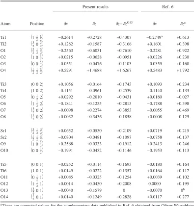
TABLE V. Atomic displacements in Å for the共2⫻1兲DL-TiO2surface. A positive value for␦z indicates

a displacement towards the vacuum. Positive␦x is in the direction of left to right in Fig. 3. Erdman et al. (Ref. 6)used a0= 3.905 Å, whereas our lattice constant is the theoretical a0= 3.85 Å.

Atom Position

Present results Ref. 6

␦x ␦z ␦z −␦zO13 ␦_x ␦_za

Ti1 共11₂ 5₂兲 −0.2614 +0.2728 +0.4307 −0.2749a +0.613 Ti2 共3₂0 5₂兲 +0.1282 +0.1587 +0.3166 +0.1601 +0.398 O1 共3_{2 2}1 5₂兲 −0.2563 +0.6031 +0.7610 −0.2281 +0.922 O2 共1 0 5₂兲 +0.0215 −0.0628 +0.0951 +0.0226 +0.230 O3 共0 0 5₂兲 −0.0551 −0.0476 +0.1103 −0.0359 +0.168 O4 共1_{2 2}1 5₂兲 +0.5291 +1.4688 +1.6267 +0.5483 +1.792

Ti3 (0 0 2) +0.1056 +0.0164 +0.1743 +0.1093 +0.234 Ti4 (1 0 2) −0.1151 −0.0961 +0.2539 −0.1140 +0.133 O5 共0₂12兲 +0.0292 −0.2010 −0.0431 +0.0180 −0.027 O6 共1₂12兲 −0.1841 +0.1235 +0.2813 −0.1788 +0.398 O7 共3₂ 0 2兲 −0.0098 +0.2274 +0.3853 −0.0055 +0.469 O8 共1₂ 0 2兲 +0.0032 −0.3436 −0.1858 +0.0008 −0.125

Sr1 共3_{2 2}1 3₂兲 +0.0652 +0.0530 +0.2109 +0.0719 +0.215 Sr2 共1_{2 2}1 3₂兲 −0.0804 −0.0481 +0.1097 −0.0758 +0.137 O9 共1 0 3₂兲 +0.2568 +0.0333 +0.1912 +0.2413 +0.246 O10 共0 0 3₂兲 −0.1991 −0.0432 +0.1146 −0.1953 +0.113

Ti5 (0 0 1) −0.0252 +0.0114 +0.1693 −0.0180 +0.164 Ti6 (1 0 1) +0.0149 −0.0222 +0.1357 +0.0164 +0.117 O11 共0₂11兲 +0.0085 −0.0325 +0.1254 +0.0039 +0.102 O12 共1₂11兲 +0.0014 +0.0430 +0.2008 0.0000 +0.195 O13 共3₂ 0 1兲 −0.0040 −0.1579 0 −0.0070 0b

O14 共1₂ 0 1兲 +0.0140 +0.1249 +0.2828 +0.0117 +0.277

a_{These are corrected values for the supplementary data published in Ref. 6 obtained from Oliver Warschkow}

via private communication.

Rather than attempting to calculate the energy E0, which

would require corrections to the classical formulas for low temperatures, as well as an accurate total energy calculation for the oxygen molecule, we again make use of experimental data. The experimental enthalpies, entropies, and Gibbs free energies per mole have been fitted to polynomials,21_namely,

H共p0,T兲− H共p0,T0兲= AT +1 2BT

2₊1

3CT

3₊1

4DT

4₋E T+ F,

共16兲

S共p0,T兲= A ln共10−3T兲+ BT +1 2CT

2₊1

3DT

3₋ E

2T2+ G, 共17兲

and

G共p0,T兲= A共T − T ln共T兲兲−1 2BT

2₋1

6CT

3

− 1 12DT

4₋ E

2T+ F − GT, 共18兲

where the coefficients are listed in Table III.

Note that the data tables give values in kJ mol−1, which we convert to Rydbergs per molecule as necessary. Hence, making use of Eq.(12), we can construct our final formula for␮O

2共pO2, T兲:

␮O₂共pO₂,T兲=␮O₂共p0,T0兲+ G共p0,T兲− G共p0,T0兲

+ kT ln

冉

p_O

2

p0

冊

Equation(19)uses as far as possible the experimental tem-perature dependence, whereas Eq.(15) was derived by as-suming an ideal classical gas of rigid dumbbells. If we fix the value of E0by the temperature derivative of the experimental

Gibbs energy at the standard temperature, the simple formula Eq. (15) does rather well: the error at 1000 K is only 0.6 kJ mol−1_{, rising to 3.5 kJ mol}−1_{共⬍3 mRy兲 at 2000 K,}

which is less than other errors in our procedure. However,

we can of course use Eq. (19) directly and avoid any ideal gas assumptions. Either formula tells us that␮O

2共p

0_{, T兲}

de-creases by 121 mRy between standard temperature 共298.15 K兲 and 1000 K, that is from −616 mRy to − 737 mRy.

IV. RESULTS AND DISCUSSION

A. Surface relaxations

For the共1⫻1兲 unreconstructed surfaces the calculations were performed on seven atomic layer supercells. The sur-face energy and atomic displacements are well converged for this size of supercell. Increasing the cell to nine atomic lay-ers only made a difference in the surface energy of 0.05 J m−2for the unrelaxed TiO2slab. Atomistic relaxation

was carried out using a Fletcher-Powell algorithm22 _{and the}

forces were converged to 0.05 mRy au−1 _{for the TiO} 2

termi-nation and 0.34 mRy au−1 _{for the SrO termination. The}

re-sults are shown in Table IV.

The agreement between our atomic displacements and those of Ref. 23 is excellent. The only atomic displacements in disagreement are those of the O1 and O2 in the SrO

ter-mination.

For the共2⫻1兲reconstructions we used slabs with mirror symmetry about the central layer of the slab. The 共2⫻1兲 Ti2O3surface was found to be metallic but nonmagnetic.

The convergence of the surface energy with the thickness of the slabs was checked by comparing the energies for 7 and 11 layer slabs and there was good agreement between the two sets of results. The atomic displacements for the 7 and 11 layer共2⫻1兲 DL-TiO2reconstruction are shown in Table

V alongside the previous results reported in Ref. 6. The atom positions are illustrated in Fig. 3. No previous results were available for comparison with the 共2⫻1兲 TiO₂ or 共2⫻1兲

FIG. 3. Vertical slices through(a)TiO₂layer and(b)SrO layer to show atom positions and labels for the 共2⫻1兲 DL-TiO2

reconstruction.

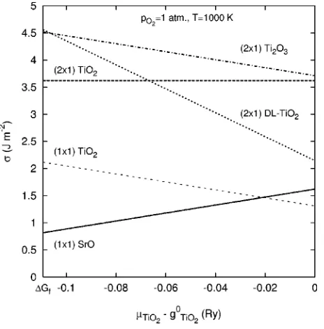
FIG. 4. Surface energies as a function of␮TiO2at T = 1000 K

Ti2O3 reconstructions. The following results for the共2⫻1兲

reconstructions were obtained using slabs with 11 atomic layers.

The agreement between our results and those of Ref. 6 is excellent. The direction of all displacements are consistent although there is some variation of magnitude. For both sets of results the Ti1-O4 bond length is considerably shorter that the bulk equilibrium bond length. Erdman et al. obtained a bond length of 1.63 Å and we obtained a bond length of 1.64 Å. The angle between the Ti1-O4 bond and the(001) plane are also in remarkable agreement. Erdman et al. ob-tained a bond angle of 46.2° and we obob-tained an angle of 46.5°.

B. Surface energies

The surface energies of the 共1⫻1兲 and 共2⫻1兲 recon-structed surfaces as a function of␮TiO

2are shown in Fig. 4. As expected from the theory, Eq. (3), the gradient of each energy is proportional to the excess of TiO₂ subunits. The 共2⫻1兲TiO2surface has the same stoichiometry as the bulk

and therefore is independent of␮TiO 2.

The surface energies of the共1⫻1兲 unreconstructed sur-faces are in good agreement with previous theory. The aver-age surface energy of these terminations is 1.46 J m−2which compares well to previous values, for example 1.35 J m−2_.23

Surprisingly the共1⫻1兲surfaces are more stable than any of the共2⫻1兲reconstructions at p0 _{and T = 1000 K. As}

pre-viously stated in the introduction one likely explanation is that the共1⫻1兲unreconstructed surfaces are not stable in an UHV experiment. To test this hypothesis we have calculated the surface energy of the 共1⫻1兲 TiO2 terminated surface

with an oxygen vacancy. For this surface we used a supercell with a共2⫻2兲unreconstructed TiO2terminated surface with

7 atomic layers and one layer of vacuum and it will be re-ferred to as the 共2⫻2兲 O vacancy surface. Similar to the 共2⫻1兲Ti2O3 reconstruction this surface is metallic.

Only the surface with the O vacancy and the 共2⫻1兲 Ti2O3 surface energies depend on pO₂ and T since they are

the only surfaces with an excess of oxygen(in these cases a negative excess or deficiency). Figures 5(a)and 5(b)show␴ vs pO₂at T = 1000 K for two different values of␮TiO₂

corre-sponding to equilibrium with TiO2and SrO, respectively.

First we consider the case where the surface is in equilib-rium with SrO. The DL-TiO2 and共2⫻1兲 TiO2

reconstruc-tions and the 共1⫻1兲 TiO₂ surface with and without an O vacancy are unstable for all values of p_O

2 shown. The 共1

FIG. 5. Surface energies as a function of p_O

2at T = 1000 K(a)in

equilibrium with TiO2and(b)in equilibrium with SrO.

⫻1兲 SrO terminated surface is predicted to be stable for partial pressures down to⬇10−68_{atm at which point the 共2}

⫻1兲 Ti2O3 surface becomes stable. If we assume that the

ideal 共1⫻1兲 surface is never obtained then the 共2⫻2兲 O vacancy surface has the lowest surface energy for partial pressures down to⬇10−48_{atm after which the共2⫻1兲Ti}

2O3

reconstruction is again stable.

Now we consider the case where the surface is in equilib-rium with TiO2. For partial pressures above⬇10−40the

per-fect共1⫻1兲 TiO2 unreconstructed surface is stable.

Neglect-ing, for now, the apparent overall stability of the 共1⫻1兲 surfaces then for p_O

2⬎10

−8 _{the DL-TiO}

2 surface is stable,

for 10−48_⬍p

O₂⬍10−8 the 共2⫻2兲 O vacancy surface is

stable, and for 10−68_⬍p

O₂⬍10−48 the 共2⫻1兲 Ti2O3

recon-struction is stable.

The pressures under consideration here are not achievable experimentally. However, it is possible to obtain extremely low effective partial pressures if a reducing agent is present. To estimate the effective partial pressures which could be

obtained we have taken as an example the case of carbon being present on the surface. Consider the thermodynamic equation for the formation of carbon dioxide from carbon and oxygen at standard temperature T0= 298 K,

C_共s兲+ O_2共g兲CO_2共g兲,

where carbon is in graphite form and CO2and O2are in the

gas phase. The Gibbs free energy balance at standard tem-perature and pressure is

␮CO

2

0

=␮C0 +␮O 2

0

+⌬Gf,CO₂, 共20兲

where⌬Gf,CO₂ is the Gibbs free energy of formation of

car-bon dioxide at standard temperature and pressure. In equilib-rium

␮CO₂共p,T兲=␮C共p,T兲+␮O

2共p,T兲 共21兲 and using the earlier derivation for the pressure dependence of the chemical potential of oxygen we can write

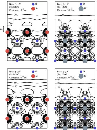
FIG. 7. (Color online)Charge densities for the 共1⫻1兲 SrO ter-minated surface for slices through the SrO and TiO2 planes in two

␮CO₂共p0,T兲+ RT ln

冉

pCO₂

p0

冊

0_,T兲

+ RT ln

冉

pO₂

p0

冊

Subtracting Eq.(20)from Eq.(22)at T0= 298 K gives

RT0_ln

冉

0

p_O

2

冊

= −⌬G_f,CO

2. 共23兲

At standard temperature RT0_{= 0.592 kcal, ⌬G} f,CO₂

= −94.15 kcal,21 _{and if the partial pressure of CO} 2

corre-sponds to UHV pressures 共⬇10−15_{atm兲, then p} O₂

⬇10−85_{atm. This simple analysis demonstrates that it is}

pos-sible to achieve low partial pressures if a reducing agent is present. In Castell’s experiment a chemical etch was used to prepare the surface and this is known to leave a carbon resi-due. This etch also serves to produce a TiO2rather than SrO

termination so Fig. 5(a)is the most appropriate to compare to these experiments. Although the surface is annealed to re-move this layer it is possible that some carbon remains which may reduce the effective partial pressure of oxygen enough to enable the共2⫻1兲Ti2O3reconstruction to become

stable.

V. IMAGE SIMULATIONS AND STM IMAGES

The question as to why the 共1⫻1兲 unreconstructed sur-faces have not been observed has not yet been answered. In this section we look at the unoccupied charge densities and make comparisons with STM imaging.

Figure 6 shows an STM image of the 共2⫻1兲 recon-structed surface. The sample bias is positive so that electrons tunnel from the metallic STM tip into the unoccupied states of the SrTiO3 specimen. The details of sample preparation

and imaging conditions are the same as those described in Ref. 4. In the lower panel of Fig. 6 a plot of the average row

height is shown. This plot shows in particular that the corru-gation height perpendicular to the rows in the image is be-tween 0.4 and 0.5 Å. The unit cell periodicity parallel to the rows cannot be resolved in the STM images.

A popular method for STM image analysis is to integrate the local density of states in an energy window around the imaging bias voltage. This method was used most notably on rutile TiO2 (110) surfaces24 and has since been applied to

other oxide surfaces, e.g., NiO and CoO.9 _{In our study we}

have integrated the empty states over two energy windows and compared the results. The windows considered, mea-sured upwards from the conduction band edge, were 0 – 1 eV and 1 – 2 eV.

A.„1Ã1…unreconstructed surfaces

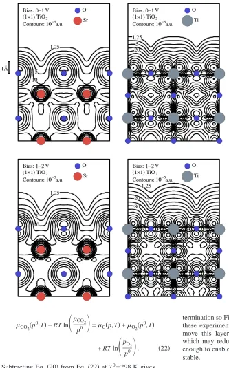
Figures 7 and 8 show the unoccupied charge densities of the 共1⫻1兲 SrO and TiO2 surfaces with slices through the

SrO and TiO2planes.

The difference between the charge densities in the two different energy windows is not significant therefore the

re-sults should not be sensitive to the sample bias.

It is interesting to note that the charge density for the SrO surface is an order of magnitude larger than that of the TiO2

surface. Even though for both surfaces the charge density around the Sr ions is much higher than around the Ti ions the contours of constant charge density on the共1⫻1兲SrO sur-face are flatter than for the 共1⫻1兲 TiO2 surface. The high

charge density around the Sr ions is in agreement with the findings of Kubo and Nozoye’s8_{calculations of their Sr}

ada-tom model. The charge density plots would therefore suggest that it is easier to obtain atomic resolution STM images from the 共1⫻1兲 TiO2 surface than from the共1⫻1兲SrO surface.

Experimental conditions such as sample bias and tunneling current would determine which charge density contours are imaged in the STM.

B.„2Ã1…reconstructions

Figures 9 and 10 show the charge densities of the 共2⫻1兲 Ti2O3 and DL-TiO2 surfaces. As for the 共1⫻1兲

re-FIG. 9. (Color online)Charge densities for the共2⫻1兲Ti2O3

ter-minated surface for slices through the SrO and TiO2 planes in two

constructions two different energy windows and slices through the SrO and TiO2 planes are shown. The 共2⫻1兲

TiO2 surface has not been considered here because its

sur-face energy is higher than the others.

The charge density for the Ti2O3 is different in the two

energy windows for the slice through the SrO layer. In the 0 – 1 eV window the corrugation is significantly larger than for the 1 – 2 eV window. Even so, the corrugation in both cases should be large enough to be imaged using STM. Sur-prisingly, the charge density of the Ti2O3 surface is higher

over the missing O row which indicates that the missing rows would be imaged rather than the rows of O atoms.

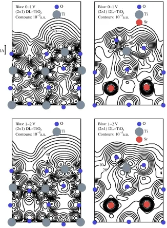
The relaxation of DL-TiO2surface can be clearly seen in

Fig. 10 including the remarkably short Ti-O bond length. In this case the regions of high charge density occur over the atoms, rather than over the missing atoms. The charge den-sity contours of the 共2⫻1兲 DL-TiO2 surface are highly

ir-regular and it should therefore be possible to image them in the STM. However, the large corrugations one sees in Fig. 10 would not be reproduced in experiment due to the

convolu-tion of the STM tip with the sample which would have the effect of reducing the corrugation heights.

The calculations show that the STM images the missing atoms for the共2⫻1兲 Ti2O3reconstruction and atomic

posi-tions for the共2⫻1兲 DL-TiO2. If one were to adsorb a

mol-ecule that attaches to the middle of the rows for both struc-tures then it would be possible to distinguish the strucstruc-tures because in the STM images the共2⫻1兲Ti₂O₃surface would show the molecule in between bright rows and the 共2⫻1兲 DL-TiO2 surface would show it on top of the bright rows.

This highlights the significance of the very different nature of the charge densities for the two proposed共2⫻1兲 recon-structions.

VI. CONCLUSIONS

We have performed first-principles total energy calcula-tions for several共2⫻1兲reconstructions of the(001)SrTiO₃ surface. The surface energies were calculated as functions of

␮TiO₂, pO₂, and T.

FIG. 10.(Color online)Charge densities for the共2⫻1兲 DL-TiO2

terminated surface for slices through the SrO and TiO2 planes

At standard pressure p0 _{and T = 1000 K the 共1⫻1兲}

sur-faces are energetically stable and all the共2⫻1兲 reconstruc-tions are unstable. The 共2⫻1兲 TiO2 reconstruction is

un-stable under all the conditions considered. Under conditions of very low pO₂ the共2⫻1兲Ti2O3 reconstruction is stable.

Charge densities for the reconstructions were calculated to investigate why the共1⫻1兲 surfaces have not been observed using STM despite the fact that they are predicted to be stable under many conditions. Of the two共1⫻1兲surfaces the TiO2-terminated surface should be easier to image than the

SrO-terminated surface. The corrugations of the charge den-sity for the 共2⫻1兲 surfaces are deeper than those for the 共1⫻1兲 surfaces and therefore the 共2⫻1兲 reconstructions should be easier to image than the共1⫻1兲.

We considered the possibility that the ideal 共1⫻1兲 sur-faces considered here do not exist in practice. In UHV con-ditions it is likely that oxygen vacancies are present. A cal-culation of the 共2⫻2兲 O vacancy surface shows that the vacancy raises the surface energy of the共1⫻1兲 surface and in some conditions it becomes higher than that of the 共2⫻1兲 reconstructed surfaces. In a TiO2-rich environment

with oxygen partial pressure greater than 10−8atm its surface energy is greater than that of the 共2⫻1兲 DL-TiO2

recon-struction and so this reconrecon-struction becomes the stable one.

In this analysis, there has been no consideration of vibra-tional entropy. Surface vibrations could contribute to the lowering of the energy. In particular, the “dangling” oxygen atoms in the DL-TiO2 surface could give rise to low

fre-quency surface vibrations which could stabilise this recon-struction.

Recently Kubo and Nozoye8 suggested that all the ob-served reconstructions could be explained using a Sr-adatom model. However no total energy calculations were carried out and without these it is impossible to compare these sur-face structures with the previous structures proposed. It would be interesting to carry out a total energy calculation of these surfaces and this may shed light on the unresolved issues.

ACKNOWLEDGMENTS

K.J. would like to thank Sasha Lozovoi for useful discus-sions and the Department for Employment and Learning, Northern Ireland for financial support. EPSRC funding was provided under Grant No. GR/R39085/01. M.R.C. is in re-ceipt of a Distinguished Visiting Fellowship of the Interna-tional Research Centre for Experimental Physics at Queen’s University.

*Present address: Department of Physics and Astronomy , Rutgers University, Piscataway, New Jersey 08854.

†_{Permanent address: Department of Materials, University of}

Ox-ford, Parks Road, Oxford OX1 3PH, United Kingdom.

1_{V. E. Henrich and P. A. Cox, The Surface Science of Metal} Ox-ides, 1st ed.(Cambridge University Press, Cambridge, 1994).

2_{Q. D. Jiang and J. Zegenhagen, Surf. Sci. 338, L882(1995).} 3_{T. Kubo and H. Nozoye, Phys. Rev. Lett. 86, 1801(2001).} 4_{M. R. Castell, Surf. Sci. 505, 1(2002).}

5_{M. R. Castell, Surf. Sci. 516, 33(2002).}

6_{N. Erdman, K. R. Poeppelmeier, M. Asta, O. Warschkow, D. E.}

Ellis, and L. D. Marks, Nature(London) 419, 55(2002).

7_{N. Erdman and L. D. Marks, Surf. Sci. 526, 107(2003).} 8_{T. Kubo and H. Nozoye, Surf. Sci. 542, 177(2003).}

9_{M. R. Castell, S. L. Dudarev, G. A. D. Briggs, and A. P. Sutton,}

Phys. Rev. B 59, 7342(1999).

10_{M. Methfessel and M. van Schilfgaarde, NFP Manual (1997),}

unpublished.

11_{Electronic Structure and Physical Properties of Solids: The Uses} of the LMTO Method; Lectures of a Workshop held at Mont Saint Odile, edited by H. Dreyssé (Springer-Verlag, Berlin 2000), pp. 114–147.

12_{A. T. Paxton and L. Thiên-Nga, Phys. Rev. B 57, 1579(1998).} 13_{D. Singh, Phys. Rev. B 43, 6388(1991).}

14_{R. D. King-Smith and D. Vanderbilt, Phys. Rev. B 49, 5828} (1994).

15_{Y. Furuhata, E. Nakamura, and E. Sawaguchi, Landolt-Börnstein,}

Group III 3(1969).

16_{R. O. Bell and G. Rupprecht, Phys. Rev. 129, 90(1963).} 17_{M. W. Finnis, Phys. Status Solidi A 166, 397(1998).}

18_{I. G. Batyrev, A. Alavi, and M. W. Finnis, Phys. Rev. B 62, 4698} (2000).

19_{A. Y. Lozovoi, A. Alavi, and M. W. Finnis, Comput. Phys.}

Com-mun. 137, 174(2001).

20_{J. Padilla and D. Vanderbilt, Phys. Rev. B 56, 1625(1997).} 21_{NIST Chemistry WebBook, NIST Standard Reference Database}

Number 69, edited by P. J. Linstrom and W. G. Mallard,( Na-tional Institute of Standards and Technology, Gaithersburg, MD, 2003), 20899 http://webbook.nist.gov/chemistry/.

22_{R. Fletcher and M. Powell, Comput. J. 6, 163(1963).} 23_{J. Padilla and D. Vanderbilt, Surf. Sci. 418, 64(1998).}

24_{U. Diebold, J. F. Anderson, K.-O. Ng, and D. Vanderbilt, Phys.}