Transduction Pathways
Thomas Millat,1 Eric Bullinger,2 Johann Rohwer,3 and Olaf Wolkenhauer1,∗ 1
University of Rostock, 18051 Rostock, Germany
2
National University of Ireland Maynooth, Co. Kildare, Ireland
3
University of Stellenbosch, 7602 Matieland, South Africa
(Dated: August 14, 2006, accepted for publication inMathematical Biosciences)
Signal transduction is the process by which the cell converts one kind of signal or stimulus into another. This involves a sequence of biochemical reactions, carried out by proteins. The dynamic response of complex cell signalling networks can be modelled and simulated in the framework of chemical kinetics. The mathematical formulation of chemical kinetics results in a system of coupled differential equations. Simplifications can arise through assumptions and approximations. The paper provides a critical discussion of frequently employed approximations in dynamic modelling of signal transduction pathways. We discuss the requirements for conservation laws, steady state approximations, and the neglect of components. We show how these approximations simplify the mathematical treatment of biochemical networks but we also demonstrate differences between the complete system and its approximations with respect to the transient and steady state behavior.
I. INTRODUCTION
The processing of information in living cells is car-ried out by signalling networks [1]. The character of information and the corresponding responses include a wide range of physical and chemical quantities, including changes in temperature, pressure, water balance, concen-tration gradients, pH-level. Within these networks infor-mation is carried by dynamic changes in protein concen-trations.
While there exist considerable experience in mathe-matical modelling of metabolic systems [2–5], cell cycle [6, 7], cellular rhythms [8, 9] and transcriptional networks (see [10, 11] for recent surveys and [12] for a recent text-book), the mathematical analysis of signal transduction pathways is a younger field [13–19]. An important dif-ference between modelling metabolic systems and signal transduction pathways is that in cell signalling one is primarily interested in the analysis of rapid responses to stimuli, oscillatory dynamics, and transient changes. A number of simplifying mathematical assumptions related to steady-state analysis are therefore not available in the analysis of signal transduction pathways.
To allow a meaningful mathematical analysis, simplifi-cations are of vital importance. It is only natural that one considers well established approximations for metabolic systems to be applicable in cell signalling. The present paper is to discuss a number of assumptions and
approxi-∗Author to whom correspondence should be addressed:
Systems Biology & Bioinformatics Group,
Faculty of Computer Science and Electrical Engineering, Albert-Einstein-Str. 21,
18059 Rostock, Germany;
Tel./Fax: +49 (0)381 498 7570/72; Email: [email protected] rostock.de;
thomas.millat@uni- rostock.de;
Internet: www.sbi.uni- rostock.de
mations that are frequently used in dynamic modelling of signal transduction pathways. We show how these sim-plify the mathematical treatment but also illustrate what happens if they are not reasonable. We demonstrate that assumptions can lead to deceptive changes in the model’s behavior. In cell signalling the choice and justification of assumptions is particularly important and relies on the experimental set-up, biological context and purpose of the model.
The outline of the paper is as follows. We begin with a description of the assumptions underlying our study, be-fore introducing activation/deactivation modules which form the basic elements of cell signalling networks. In Sections III to VI, we introduce commonly used approxi-mations and simplifications, including assumptions about stationarity assumptions, conservation and moiety laws, and the neglect of components. In Section VII, the appli-cation and consequences of assumptions and approxima-tions are demonstrated for a MAPK cascade. This leads us to a discussion of simplifications in the description of feedback mechanisms.
II. ASSUMPTIONS OF THE STUDY
For the present paper we treat a signal transduction pathway as a network of coupled modules, as illustrated in Figure 1 [20, 21]. For each activation/deactivation cycle an enzyme kinetic reaction serves as a template:
X + E k1
−−−* )−−−
k−1
C k2
−→E + X∗ (1)
en-(a) K
X X∗
(b) K
Y
X X∗
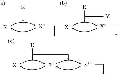
(c) K
[image:2.612.73.269.59.182.2]X X∗ X∗∗
FIG. 1: Modules (of activation/deactivation cycles) of which signal transduction pathways are composed.
zyme in (1) is a kinase for activation and a phosphatase for deactivation.
A standard approach to the dynamics of cell signalling networks is the framework of chemical kinetics. Within this framework enzyme kinetic reaction (1) is represented as a system of four coupled ordinary differential equations [11, 22]
dX
dt = −k1EX+k−1C , (2) dE
dt = −k1EX+ (k−1+k2)C , (3)
dC
dt = k1EX−(k−1+k2)C , (4) dX∗
dt = k2C . (5)
Such a system of rate equations can be generalized to the following form [2]
dSi
dt =
m
X
µ=1
νµikµ
Y
j
Slµj
j , i= 1, . . . , n , (6)
whereνµi is the stoichiometric coefficient, which is
posi-tive for synthesis and negaposi-tive for degradation, andlµi is
the reaction order. The reaction rate is proportional to the concentration of reaction partners and rate coefficient
kµ.
There is a no such thing as a hypothesis-free model and before we discuss various approximations that de-rive from the basic modification scheme (1), we ought to mention the assumptions that are implicitly made to this point. The approach has been originally derived from microscopic properties in statistical physics [23]. It links the rate of change of a component Si to an average
num-ber of reactive collisions in a reaction volume. Eq. (6) therefore implies the assumption that a mean value is an appropriate description for changes in protein con-centrations; random fluctuations (noise) are considered small in comparison to this mean [23]. In that respect, Eq. (6) describes ‘macroscopic’ changes of protein con-centrations. A fundamental assumption of this approach is a homogeneous distribution of all components in the
reaction volume. Diffusion processes are assumed to be much faster than the chemical reaction made responsible for the signalling mechanism. We stay therefore in the realm of ordinary differential equations, not partial differ-ential equations. Assuming that environmental variables (e.g. temperature and volume) do not change, kµ is a
reaction constant.
III. STATIONARY COMPONENTS
In case of (de)phosphorylations, the reaction schema (1) ignores the involvement of ATP. This simplification is made possibly by assuming that ATP is available ei-ther in great excess or can be supplied without significant changes in concentration. This assumption is frequently used for ATP in the activation cycles of Figure 1 [26].
We can illustrate this with a more detailed model
X+E k1
−−−* )−−−
k−1
C
C+ATP k
0 2
−→ X∗+E+ADP .
(7)
In a first reaction step, enzyme and protein X form a complex C, which is the target for the ATP molecule. The reaction between the complex and ATP activates the protein and release the unchanged enzyme E and ADP. The corresponding differential equation for the rate of change of the active protein is now
dX∗
dt =k
0
2ATP C .
If we assume a stationary ATP concentration we can in-troduce an effective or apparent rate constant
k2=k20ATP
leading to a differential equation, equivalent to (5). In the same manner the other differential equations of reac-tion scheme (7) can be reduced to a formally equivalent system of (2)-(5). The effective rate constantk2depends on the ATP concentration. Experiments with different ATP levels will subsequently lead to a different dissoci-ation constants k2. This underlines the importance for monitoring the concentration of stationary components. The identification of a parametric dependence of a rate coefficient on other species is an indication for a more complex reaction mechanism.
IV. CONSERVATION LAWS, MOIETY LAWS
A further simplification in the treatment of signalling pathways arises if some components obey conservation relations with respect to the number of molecules in-volved. Moving from molecule numbers to concentra-tions, so-called moiety laws are defined. For example, in case of the reaction scheme (1) we can assume
where ET is the total enzyme concentration, composed of the free enzyme concentration E(t) and the enzymes bound in the intermediate complex C. During the course of the reaction, the ratio of enzyme and enzyme-substrate complex is changing, but their sum remains constant over time. Conservation relation (8) allows us to replaceE(t) in other equations by ET−C(t) and thereby to reduce the overall number of differential equations. This idea is frequently used [13, 26–28].
A notable difference between metabolic networks and signalling pathways is the fact that the latter can often be considered a closed system, restricted by the cell mem-brane. In closed systems the conservation relation is an exact relation and has no consequences on the dynamic behavior. Even if the system as a whole is open, it can be closed with respect to some components.
V. QUASI-STEADY STATE APPROXIMATION
Within the modules of Figure 1 elementary reac-tions produce short-lived intermediates, like the enzyme-substrate complex in Eq. (1). This is then referred to as a pre-equilibrium [24], in which an intermediate is in equi-librium with the reactants. This is only possible if the rate of formation for an intermediate and its dissociation back into the reactants is much faster than its conversion into products [24]. For complex C this quasi-steady state assumption leads to a simplification in Eqs. (2)-(5)
dX∗
dt =− dX
dt =k2C(t) =k2
X(t)E(t)
KM
. (9)
The Michaelis-Menten scheme now formally follows a pseudo-bimolecular rate law. Such a reduction of the underlying mechanism is a characteristic property of the quasi-steady state approximation.
If we further use conservation relation (8) we obtain the well-known Michaelis-Menten equation [3, 27, 29, 30]
dX∗
dt =− dX
dt =
VmaxX
KM+X
, (10)
with the limiting rate Vmax=k2ET and Michaelis con-stantKM= (k−1+k2)/k1. The conditions for the appli-cation of the quasi-steady state assumption were gener-alized in [31, 32]. A generalization to reversible enzyme kinetics is given in [33].
Instead of the three rate coefficientsk1,k−1, andk2 of complete model (2)-(5) the Michaelis-Menten equation (10) is parametrically dependent on two new coefficients, which can often be measured in experiments. Because the original rate coefficients cannot be uniquely determined from the limiting rateVmax and Michaelis constantKM, the quasi-steady state assumption leads to a loss of in-formation about the reaction mechanism. Note, that the rational form of the Michaelis-Menten equation is a con-sequence of (8).
time t/τ
N
o
rm
a
li
ze
d
co
n
ce
n
tr
a
ti
o
n
s
I II III
substrate product
enzyme complex
k1=10 k−1=0.5
k2=17
100−2 10−1 100 101 102 103 104
[image:3.612.337.535.55.214.2]0.2 0.4 0.6 0.8 1
FIG. 2: Comparison of the integrated Michaelis-Menten equa-tion (10) (dashed) and the numerical soluequa-tion of the system of coupled ODE’s (2)-(5) in a semilogarithmic representation. In addition to the evolution of protein X and its modified form (solid lines) proteins, the enzyme and complex concen-trations are shown as a function of time. The concenconcen-trations are normalized to the initial protein concentrationX0. The time axis is scaled with the characteristic timeτ (11). The dynamics are separated into three parts: I - initial period, II - period of quasi-steady states, III - final stage.
In Figure 2, we compare the solution for the full system of coupled differential equations with its approximate de-scription (10). In order to illustrate all three phases of the reaction we choose a normalized logarithmic time scale. As the scale factor we use the characteristic time needed to establish the quasi-steady state [34]
τ = (k1X0+k−1+k2)−1 . (11) Apart from dissociation constantsk−1andk2,τdepends on the formation of complex C described by the associ-ation ratek1 and the initial substrate concentrationX0. During this initial period the Michaelis-Menten equa-tion deviates from a detailed model, especially for the temporal evolution of the substrate. During phase (II), 1< t/τ <300, the enzyme complex is saturated due to the limited amount of enzyme. This is the region, where the quasi-steady state assumption is valid. Due to the ratio of enzyme and substrate in Figure 2, the tempo-ral evolution of the substrate is not well described by the Michaelis-Menten equation, although in period (II) a quasi-steady state of the enzyme-substrate complex C is established. If the ratio becomes small (X0E0), devi-ations occurring from the initial period can be neglected. Towards the end, in phase (III), the enzyme complex is degrading because of the lack of substrate leading to a decrease of the formation rate. The assumption of an equilibrium between complex and reactants is no longer valid and the two models differ in their transient behav-ior.
10−2 10−1 100 101 102 0
0.2 0.4 0.6 0.8 1
V1/V2
X
∗SS
/
X
T
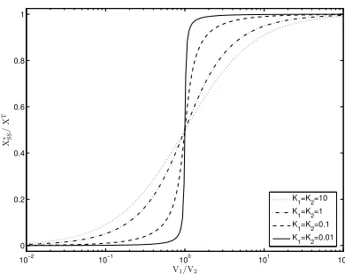
[image:4.612.77.272.54.209.2]K1=K2=10 K1=K2=1 K1=K2=0.1 K1=K2=0.01
FIG. 3: The Goldbeter-Koshland functionG(V1, V2, K1, K2) (16) as function of the ratio of limiting ratesV1 andV2. The
normalized steady state concentrationX∗/XT
is plotted for the symmetrical modification cycle (K1 =K2). Depending on the values of the Michaelis constants, the Goldbeter-Koshland function can show sigmoidal or ultrasensitive behavior.
condition for the approximation of a quasi-steady state. The Michaelis-Menten equation (10) and the enzyme kinetic reaction Eqs. (2)-(5) have a similar long-term behavior, but they deviate in the short-term behavior. Thus, the underlying quasi-steady state approximation may be applicable in metabolism, but can be problematic in signalling, where we are interested in the description of fast transient changes beyond the steady state. We are going to further discuss Michaelis-Menten modelling below. For a discussion of this modelling approach with applications in cell signalling see [36].
VI. NEGLECTING COMPONENTS
In order to simplify the mathematical treatment of (de)activation cycles (Figure 1), one often uses a
combi-nation of the previous discussed approximations. First, one can decompose the modification and the reverse process into two separate Michaelis-Menten-type reac-tions, where we assume, that additional participants are constant (See Section III) and obtain the reaction scheme
X + E1
k1
−−−* )−−−
k−1
C1
k2
−→E1+ X∗ X∗+ E
2
k3
−−−* )−−−
k−3
C2
k4
−→E2+ X.
(12)
With the conservation laws for the kinase E1 and the phosphatase E2, analogous to (8), for the protein
XT=X(t) +X∗(t) +C1(t) +C2(t), (13) and the quasi-steady state approximation for the formed complexes C1 and C2 we obtain an expression which in-volves the complex concentrations. If we assume, that the concentration of the complexes C1 and C2 are much smaller than the concentration of the modified protein X∗ and its original form X
X+X∗C
1+C2. (14)
we can neglect their contributions in conservation law (13). Because the maximal concentration of complexes is determined by the enzyme, from (14) the enzyme con-centration must be small. We thus obtain the following rate equation [26]
dX∗/XT
dt =
1
XT
V
1(1−X∗/XT)
K1+ 1−X∗/XT
− V2X
∗/XT
K2+X∗/XT
(15)
with the limiting ratesV1=k2E1TandV2=k4ET2 and the dimensionless Michaelis constantsK1= (k−1+k2)/(k1XT) andK2= (k−3+k4)/(k3XT). The corresponding steady state is described by the Goldbeter-Koshland function [26]
G(V1, V2, K1, K2) =
X∗ SS
XT =
V1(1−K2)−V2(1 +K1) +
q
[V1(1−K2)−V2(1 +K1)]2+ 4V1K2(V1−V2) 2(V1−V2)
, (16)
having a characteristic sigmoidal shape as a function of the ratio of the limiting rates, see Figure 3. Roughly speaking, the ratio of kinase to phosphatase defines a switch-like behavior which depends on the Michaelis con-stants. The steady state concentration of X∗ increases abruptly from a low (nearly zero) concentration to a high level (nearlyXT). Such behavior is called ‘ultrasensitiv-ity’ [26, 28]. Apart from the described covalent mech-anism, referred to as zero-order ultrasensitivity, other mechanisms leading to ultrasensitive behavior have been
0 20 40 60 80 100 0
0.2 0.4 0.6 0.8 1
time
X
∗/
X
T
ET=0.25
ET=0.05 ET=0.1
k1=5
k−1=2 k2=1
k3=2
[image:5.612.355.527.56.233.2]k−3=0.5 k4=0.1
FIG. 4: Temporal evolution of modified protein X∗ to its
steady state for different enzyme concentrations. The solid lines are the solution for finite enzyme concentrations and the dashed lines the corresponding solution of (16).
10−3 10−2 10−1 100
0.1 0.2 0.3 0.4 0.5 0.6 0.7 0.8
ET/ XT
X
∗/
X
T
V1/V2=2
V1/V2=1.5
V1/V2=1
V1/V2=2/3
V1/V2=0.5
k1=5 k−1=2
k2=1
k3=5 k−3=2
[image:5.612.79.272.59.208.2]k4=1
FIG. 5: Steady state concentration of modified protein X∗
as function of the ratio of catalyzing enzyme concentration and total protein concentration XT
for different ratios of the limiting rates V1 and V2. For small ratios the enzyme-substrate complex can be neglected in the protein balance and the steady state tends asymptotically to result of Goldbeter-Koshland [26] (dashed lines).
steady state for the modified form deviates from Eq. (16). The differences in the steady state values increases with the ratio of enzyme and protein concentration, as one could expect. Additionally, a further increase comes with the ratio of the limiting ratesV1/V2, as demonstrated in Figure 5.
Whereas assumption (14) holds true for most
in-vitro enzyme reactions, it often fails in
phosphoryla-tion/dephosphorylation reactions in signalling pathways. In signal transduction the concentration of substrate, ki-nase and phosphatase can be comparable [15, 37, 38]. As a consequence of the decreased steady state, the sig-moidal shape is stretched and thereby the ultrasensitiv-ity. With an increased enzyme concentration, the switch-like ultrasensitive behavior can disappear [36].
E1
W 2 1 W∗
X 4 3 XP
XPP
6 5
Y 8 7 YP
YPP
10 9
FIG. 6: Schematic representation of the basic MAPK cascade. The activated protein of the previous level acts as a kinase of the subsequent one. The dashed lines denote an implicit feed-back from the upstream level feed-back to their precursor through the released activated proteins if the complexes dissociate. A possible negative feedback loop (e.g. [28]) is denoted by a dot-ted line. There is a specialized phosphatase for each protein. As for the phosphorylation we assume for the dephosphoryla-tion that the kinetic parameters are independent on the status of protein activation (non-, single- or double-phosphorylated). Each (de)activation stepiis determined by the rate constants
aidescribing the formation of complexes,didescribing the
re-verse reaction, andkidescribing the dissociation into product
and enzyme.
VII. SIGNALLING CASCADES
An example for a sequence of (de)activation cycles is the MAPK cascade [20](Figure 6). MAPK cascades have been modelled by various authors [13–17, 28, 37–40, 44]. We will show in this section that these models result from different levels of approximation within a common funda-mental reaction scheme. Considering some components of the fundamental model we will discuss a step-by-step reduction of the model and its consequences on dynamics. The starting point is the mechanistic model of Huang & Ferrell [13] which was also used in [14, 15, 39, 40]. Note, that the first assumption in all cited papers was that the concentrations of additional participants (ATP, H2O,...) are constant. As described in Section III, we can then use the enzyme kinetic reaction as a template for the (de)phosphorylation processes in the cascade. A model reduction occurs if we use the conservation relations for the phosphatases and the kinase E1[13] and for the pro-teins which contain the different protein forms and all related complexes. In [28] these complexes are neglected. However, the conservation of phosphatases of proteins X and Y do not follow the conservation relation (8). In-stead of we have
ET=E(t) +CP(t) +CPP(t), (17)
[image:5.612.79.274.284.437.2]phos-phatase and the different phosphorylated protein forms. In contrast to the single activation/deactivation cycle, the rate equations of the cascade proteins are more com-plex as shown in Eq. (18) for the double phosphorylated protein XPP. The active protein W∗acts as a kinase and the enzyme E4 is the corresponding phosphatase. The formation of complexes is proportional to the rate con-stantsai, the reverse reaction todi, and the dissociation
into product and enzyme to the constants ki. The
un-derlined terms in (18) correspond to the ‘implicit feed-back’, which describes the freed kinases in the modifica-tion process. Due to this ‘implicit feedback’ downstream activation steps also influence the dynamics of the previ-ous steps. In Figure 6 this is shown with dashed lines.
dXPP
dt =k5C
XP
W∗−[a6E4+a7Y +a9YP]XPP (18)
+ d6CX PP
E4 + [d7+k7]C
XPP
Y + [d9+k9]CX
PP
YP ,
whereCdenotes the formed complex with the protein as superscript with kinase. Besides the ‘implicit feedback’, see also [41], the enzyme involved in the (de)activation leads to an ‘implicit inhibition’ [42, 43]. For instance, the single-phosphorylated protein XP inhibits the phospho-rylation of X and X inhibits the phosphophospho-rylation of XP through the competition for W∗. An analogues inhibi-tion mechanism exists for the dephosphorylainhibi-tion of the proteins in the cascade.
A further simplification arises if one uses the quasi-steady state approximation for the formed complexes. The system of 30 coupled differential equations can then be reduced to eight equations involving only the proteins. Not only the number of equations is reduced , the struc-ture of the equations is simplified as well. For instance rate equation (18) reduces to
dXPP
dt =k5C
XP
W∗−k6CX
PP
E4 , (19)
where the rate is now determined by the slowest step of phosphorylation and dephosphorylation. From the dis-cussion in Section V, these slowest steps have to be the dissociation of the formed enzyme-substrate complex. As shown in (9), Eq. (19) can also be expressed in terms of pseudo-bimolecular reactions, leading to the representa-tion of Heinrich et al. [17]. A comparison of Eqs. (18) and (19) shows that the reduced rate equation does not contain any implicit feedback. Therefore the dynamics of both representations will differ if the implicit feedback becomes important (i.e. whenever the steady state as-sumption is not satisfied).
Due to conservation relations, Eq. (19) can be trans-formed into rational expressions of the rate laws. On the other hand, the phosphatases of proteins X and Y sup-port conservation relation (17), which does not allow an analogue transformation as discussed in Section V. In or-der to further simplify the rate laws of these phosphatases
we assume
ET+CP(t)CPP(t) single phosphorylated,
ET+CPP(t)CP(t) double phosphorylated.
These conditions can be fulfilled simultaneously only if
ET
CP(t) +CPP(t) (20)
for the phosphatases. In contrast to the treatment of the enzyme kinetic reaction, the phosphatases are not sat-urated during the steady state phase. The quasi-steady state expression of the protein-protein complexes are obtained if we assume that the complex concentra-tions are negligible. Only the current complex remains in the expression. After some transformation we obtain Goldbeter-Koshland like rate laws for the proteins in the cascade. For example, we have for the double phospho-rylated signalling protein XPP
dXPP
dt =
k5XPW∗
KM5+XP
− k6E
T 4 XPP
KM6+XPP
,
whereKM5,6 are the corresponding Michaelis constants. Note, that we substitute the conservation law term in the above equation (see for example the dynamic Goldbeter-Koshland function (15)). Such a representation was used for instance in [28, 44].
(a)
R S
E E∗
(b)
R S
[image:7.612.341.540.55.212.2]E∗ E
FIG. 7: Diagrammatic representation of a homoeostatic sys-tem (a) and a mutually activated syssys-tem (b) according to [45].
Furthermore, the assumption of a quasi-steady state for the intermediate complexes is crucial. If substrate concentration and the modifying enzyme concentration are similar, a small rate coefficientk2is the consequence. Furthermore an enzyme saturation is, either not reached or only for a short time.
VIII. QUASI-STATIONARY STATES IN
FEEDBACK MECHANISMS
The behavior of signalling networks is regulated and controlled by positive and/or negative feedback. It is often assumed that the reactions involved in the feed-back loops are much faster than the regulated branch of the network (e.g. in the cell cycle [6, 7]). In this case, the component feeding back can be treated as a steady state variable. The regulated component is assumed as approximately constant, or quasi-stationary, during the period needed to establish the steady state of the feed-back loop. The changes in the dynamics of a system due to the applied quasi-stationary approximation shall be discussed in this section. We consider simple models consisting of a linear reaction scheme, which is regulated in an autocatalytic manner through an enzyme having an active and an inactive form.
For the first example, we use a minimal model for a homoeostatic system, shown in Figure 7. The signalling component R is synthesized in a catalytic reaction and degraded in a bimolecular reaction with an external con-stant stimulus S
dR
dt =k0E−k2SR . (21)
The enzyme dynamics follow the modification scheme (12). In Figure 8 we compare the dynamical treatment
dE dt =
k3(1−E)
KM3+ 1−E
− k4ER KM4+E
(22)
with the quasi-stationary model published in [45], where the enzyme E is assumed in its steady state
E(R) =G(k3, k4R, KM3, KM4). (23)
Due to the negative feedback, the system can display damped oscillations. The dynamic description of the
0 5 10 15 20
0 0.2 0.4 0.6 0.8 1 1.2
time
R
(t
)
k0=1 k2=1
KM3=0.01
KM4=0.01 ET=1
[image:7.612.84.268.55.150.2]k3=k4=0.1⋅k0 k3=k4=k0 k3=k4=10⋅k0 qs approximation
FIG. 8: Temporal evolution of the homoeostatic model [45] for the quasi-stationary approximation of enzyme activation (23) and the detailed model (22). Due to a negative feedback loop, the detailed model shows damped oscillations, which are dependent on the ratio of the rate coefficients. Only, if the enzyme activation cycle reaches its equilibrium rapidly, both models agree. For a very slow relaxation, the curve shows aperiodic behavior and takes much longer to equilibrate as is predicted by the quasi-stationary model.
feedback loop leads to a qualitatively different dynamic behavior than the model using the quasi-stationary ap-proximation, which cannot show oscillations. Note that the steady state is unaffected because the individual steady states of the subsystems remain unaffected. In a more complex signalling network this can lead to a qualitatively new behavior of the system as a whole. For example, damped oscillations may occur or thresholds (bifurcation points) may be passed. The faster the en-zyme activation in comparison to the synthesis of the sig-nalling component R, the smaller the deviations between a detailed and the quasi-stationary model.
In addition to a change in the dynamics of a signal, the quasi-stationary state assumption can affect other characteristic properties of biochemical networks. As an example, we consider the model of a one-way switch (Fig-ure 7(b)) discussed in [45]. The behavior of this system is linked to biological processes for which a fundamen-tal, possibly irreversible decisions between two states are made. This is, for instance, the case in cell differentiation and in developmental processes [46–48]. The synthesis of the signalling component R
dR dt =k0E
∗+k
1S−k2R (24)
is increased by the modified enzyme E∗. Enzyme modifi-cation is controlled by the signalling component R itself. Again, we compare the dynamic model
dE∗
dt =
k3(1−E∗)R
KM3+ 1−E∗
− k4E
∗
KM4+E∗
(25)
with the quasi-stationary approximation
E∗(R) =G(k
time t
re
sp
o
n
se
R
S=11 S=20
k0=1
k1=1 k2=1 ET=1
k3=1
k4=1 KM3=0.01 KM4=0.01
0 10 20 30 40 50
0 0.1 0.2 0.3 0.4 0.5 0.6
1 2 3 4
0 10 20 30 40
stimulus S/Scrit
si
g
n
a
l
d
u
ra
ti
o
n
∆
τ dynamic quasi−stationary
FIG. 9: Relaxation of the one-way switch (24) to steady state for two different, constant supercritical stimuli in quasi-stationary approximation (dashed) and in dynamic treatment (solid). The horizontal line marks the concentration which has to be exceeded for the system to reach to the upper sta-ble branch after the external stimulus is switched off. In the grey region no stable steady state solution exists. The inset shows the critical signal duration time ∆τ as function of the stimulus for both approximations.
(a)
R
S (b) S
[image:8.612.80.274.55.208.2]R R∗
FIG. 10: Diagrammatic representation of a linear (a) and a hyperbolic system (b) [45].
Whereas both models show a similar dynamic behavior (see Figure 9), some characteristic times differ. An im-portant time for a bistable system is the signal duration ∆τ needed to reach the upper stable branch, if the super-critical external stimulus is switched off after ∆τ. This characteristic time is compared in the inset of Figure 9. In the quasi-stationary approximation the steady state is reached much faster than in a dynamical model. Espe-cially for small supercritical signals the signal duration deviates from each other.
Note, in Figure 8 we vary the rate coefficients deter-mining the subsystems; a more general measure for this purpose is the relaxation timeτ. This characteristic time is a measure for the time the biochemical reaction needs to relax from a perturbated state to its steady state. Es-pecially for complex signalling networks this is not only dependent on the rate coefficientskµ, but also on the
con-centrations of other participating species. For instance, the relaxation time of a simple linear system (Figure 10(a)) is
τlin=k2−1, (27)
that is, the inverse of the degradation rate constant k2. If we consider a hyperbolic system (Figure 10(b)), the
relaxation time is
τhyb= (k2+k1S)−1 , (28) whereSis the external stimulus. A change in the concen-tration thus varies the ratios of the relaxation times. Un-fortunately, the estimation of characteristic times is ex-ceedingly difficult if no analytical expressions are known [49].
A more detailed description of feedback loops can change the dynamic behavior of the system and its char-acteristic parameters in comparison to a quasi-stationary approximation, whereas the steady state is unchanged. The approximation of a quasi-stationary state may ap-ply if one subsystem settles into a steady state much faster than the other. One must however be aware that the ratio of the relaxation times depends on the current conditions of the considered system. For the dynamic modelling of signalling networks this approximation has to be validated for each model.
IX. DISCUSSION
The framework of chemical kinetics is a frequently used approach to dynamic modelling of complex signalling net-works. The resulting systems of coupled ordinary non-linear differential equations can usually only be solved numerically. To reduce the complexity of an analysis, one uses exact relations, like conservation relations, and different approximations like steady-state assumptions or one neglects components. Such a reduction simplifies the mathematical dimension of biochemical networks and makes the model amenable to the estimation of parame-ter values from experimental data. The downside is that an approximation can misguide the analysis of the real dynamical behavior of the pathway.
As shown in Section V, the time until reaching a steady state can bring about further differences between the pre-dicted time course and the one observed in experiments. A similar conclusion can be drawn if a quasi-stationary state approximation is used, e.g. for a feedback loop. The altered behavior of this single subunit of the model can change the behavior of the system as a whole. It can happen that this loop induces oscillations into the net-work or the unstable region is shifted to other external stimuli.
Furthermore a comparison of model parameters is dif-ficult due to the uncertainty in determining rate coef-ficients from Michaelis constants. Due to the possible changes in the dynamic behavior, the set of parameters of a detailed model must be derived from experimental data.
[image:8.612.89.257.327.376.2]the treatment of feedback loops one has to take care us-ing these approximations. Small changes in the dynamics of the loop can change the overall behavior substantially. Common for the steady-state approximations are, that they do not influence the steady state value. In contrast, the neglect of the finite concentration of intermediates, influences the steady-state values and leads to a weaken-ing or disappearance of ultrasensitive characteristics. In signalling cascades consisting of a combination of activa-tion/deactivation cycles, even small changes in the ultra-sensitivity can change the overall behavior. Furthermore, pathways are often regulated by multiple feedback loops. Hence, the combination of steady-state assumptions and neglect of components may result in very different dy-namics.
As shown in Section VI, each activation cycle can show ultrasensitive behavior depending on the associated Michaelis constants and the ratio of the ‘substrate’ pro-tein and the kinase. A weakening or disappearance of ultrasensitivity, due to finite complex concentrations in the cycles, can change the behavior of the whole cascade qualitatively. For the same set of parameters (Michaelis constants and limiting rates) the amplification, possi-ble oscillations or multistability can change dramatically. Notice, one ultrasensitive step in the cascade is enough
to create such nonlinear behavior.
Whereas steady state properties are more robust against approximations, the dynamic behavior is sensi-tive to the approximations used. Hence, if transient, dy-namic behavior is most relevant, (e.g. in cell signalling) some frequently used approximations have to be justified. Finally, what we have shown is that dynamic pathway modelling requires careful considerations with regard to the role of mathematical models in explaining observa-tions, hypothesizing phenomena and supporting the de-sign of experiments: Systems biology is theartof making
appropriate assumptions.
Acknowledgments
T.M. and O.W. acknowledge the support of the German Federal Ministry of Education and Research (BMBF) grant 01GR0475 as part of the National Genome Research Network (NGFN). Parts of this work were supported by an EU FP6 grant LSHG-CT-2004-512060 within the project Computational Systems Biol-ogy of Cell Signalling(COSBICS). The responsibility for the content lies with the authors.
[1] Downward, J. (2001) The ins and outs of signalling, Na-ture411(6839), 759-762.
[2] Heinrich, R. and Schuster, S. (1996) The Regulation of
Cellular Systems, Chapmann & Hall, New York.
[3] Cornish-Bowden, A. (1995)Fundamentals of Enzyme
Ki-netics, Portland Press, London.
[4] Fell, D. (2003)Understanding the Control of Metabolism, Portland Press, London.
[5] Schilling, C.H., Schuster, S., Palsson, B.O., Heinrich, R. (1999) Metabolic pathway analysis: basic concepts and scientific applications in the post-genomic era, Biotech-nol. Prog.15(3), 296-303.
[6] Chen, K.C., Csikasz-Nagy, A., Gyorffy, B., Val, J. Novak, B., and Tyson, J.J. (2000) Kinetic Analysis of a Molec-ular Model of the Budding Yeast Cell Cycle, Mol. Biol. Cell11(1), 369-391.
[7] Novak, B., Pataki, Z., Ciliberto, A., and Tyson, J.J. (2001) Mathematical model of the cell division cycle of fission yeast, Chaos11(1), 277-286.
[8] Goldbeter, A. (1996) Biochemical Oscillations and
Cel-lular Rhythms, Cambridge University Press, Cambridge.
[9] Winfree, A.T. (2001)The Geometry of Biological Time, Springer Verlag, New York.
[10] De Jong, H. (2002) Modeling and Simulation of Genetic Regulatory Systems: A Literature Review, J. Comp. Bi-ology9(1), 67-103.
[11] Crampin, E.J., Schnell, S., and McSharry, P.E. (2004) Mathematical and computational techniques to deduce complex biochemical reaction mechanisms, Prog. Bio-phys. & Mol. Biol.86(1), 77-112.
[12] Fall, C.P., Marland, E.S., Wagner, J.M., Tyson, J.J. (Eds.) (2002)Computational Cell Biology, Springer
Ver-lag, New York.
[13] Huang, C.-Y.F. and Ferrell, J.E., Jr. (1996) Ultrasensi-tivity in the mitogen-activated protein kinase cascade, PNAS93(19), 10078-10083.
[14] Asthagiri, A.R. and Lauffenburger, D.A. (2001) A Com-putational Study of Feedback Effects on Signal Dynamics in a Mitogen-Activated Protein Kinase (MAPK) Path-way Model, Biotechnol. Prog.17(2), 227-239.
[15] Schoeberl, B., Eichler-Jonsson, C., Gilles, E.D., and M¨uller, G. (2002) Computational modeling of the dy-namics of the MAP kinase cascade activated by surface and internalized EGF receptors, Nature Biotech.20(4), 370-375.
[16] Ferrell, J.E. Jr. and Bhatt, R.R. (1997) Mechanistic Studies of the Dual Phosphorylation of Mitogen activated Protein Kinase, J. Biol. Chem.272(30), 19008-19016. [17] Heinrich, R., Nell, B.G., and Rapoport, T.A. (2002)
Mathematical Models of Protein Kinase, Mol. Cell9(5), 957-970.
[18] Swameye, I., M¨uller, T.G., Timmer, J., Sandra, O., and Klingm¨uller, U. (2003) Identification of nucleocyroplas-mic cycling as a remote sensor in cellular signaling by databased modeling, PNAS100(3), 1028-1033.
[19] Timmer, J., T.G. M¨uller, Swameye, I., Sandra, O., and Klingm¨uller, U. (2004) Modeling the Nonlinear Dynam-ics of Cellular Signal Transduction, Int. J. Bifurcation & Chaos14(6), 2069-2079.
[20] Lewis, T.S., Shapiro, P.S., and Ahn, N.G. (1998) Sig-nal Transduction through MAP Kinase Cascades, Adv. Cancer Res.74, 49-139.
and Regulation of IntraCellular Networks, FEBS Letters 579(8), 1846-1853.
[22] Wolkenhauer, O. and Mesarovic, M. (2005) Feedback Dy-namics and Cell Function: Why Systems Biology is called Systems Biology, Molecular BioSystems1(1), 14-16. [23] Fowler, R. and Guggenheim, E.A. (1952) Statistical
Thermodynamics, Cambridge University Press,
Cam-bridge.
[24] Atkins, P. and de Paula, J. (2002)Atkins’ Physical
Chem-istry, Oxford University Press, Oxford.
[25] H¨anggi, P., Talkner, P., and Borkovec, M. (1990) Reaction-rate theory: fifty years after Kramers, Rev. Mod. Phys.62(2), 251-341.
[26] Goldbeter, A. and Koshland, D.E., Jr. (1981) An am-plified sensitivity arising from covalent modification in biological systems, PNAS78(11), 6840-6844.
[27] Segel, I.H. (1993)Enzyme Kinetics: Behavior and Analy-sis of Rapid Equilibrium and Steady-State Enzyme Sys-tems, Wiley, New York.
[28] Kholodenko, B.N. (2000) Negative Feedback and ultra-sensitivity can bring about oscillations in the mitogen-activated protein kinase cascades Eur. J. Biochem.267 (6), 1583-1588.
[29] Mathews, C.K., van Holde, K.E., and Ahern, K. (2000)
Biochemistry, Benjamin/Cummings, San Fransisco.
[30] Michaelis, L. and Menten, M.L. (1913) Die Kinetik der Invertinwirkung, Biochem. Z.49, 333-369.
[31] Briggs, G.E. and Haldane, J.B.S. (1925) A note on the kinetics of enzyme action, Biochem. J.19, 338-339. [32] Schnell, S. and Mendoza, C. (1997) Closed Form
So-lution for Time-dependent Enzyme Kinetics, J. Theor. Biol.187(2), 207-212.
[33] Tzafriri, A.R. and Edelmann, E.R (2004) The total quasi-steady state approximation is valid for reversible enzyme kinetics, J. Theor. Biol. 226(3), 303-313.
[34] Rubinow, S.I. (2003)Introduction to Mathematical Biol-ogy, Dover Publications, Mineola (N.Y.).
[35] Cox, B.G. (1994)Modern Liquid Phase Kinetics, Oxford University Press, Oxford.
[36] Bl¨uthgen, N., Bruggeman, F.J., Legewie, S., Herzel, H., Westerhoff, H.V., Kholodenko, B.N. and Sauro, H.M. (2006) Sequestration affects ultrasensitivity in signal transduction cascades, FEBS Journal237(5), 895-906. [37] Ferrell Jr., J.E. (1996) Tripping the switch fantastic: how
a protein kinase cascade can convert graded inputs into switch-like outputs, TIBS21(12), 460-466.
[38] Yeung, K., Seitz, T., Li, S., Janosch, P., McFerran, B., Kaiser, C., Fee, F., Katsanakis, K.D., Rose, D.W.,
Mis-chak, H., Sedivy, J.M., Kolch, W. (1999) Supression of Raf-1 kinase activity and MAP kinase signalling by RKIP, Nature401, 173-177.
[39] Cho, K.-H., Shin, S.-Y., Kim, H.-W., Wolkenhauer, O., McFerran, B., and Kolch, W., Mathematical Modelling of the Influence of RKIP on the ERK Signalling Pathway (2003) Computational Methods in Systems Biology, Ed. Priami, C., Springer Verlag, 127-141.
[40] Brightmann, F.A and Fell, D.A. (2000) Differential feed-back regulation of the MAPK cascade underlies the quan-titative differences in EGF and NGF signalling in PC12 cells, FEBS Lett.482(3), 169-174.
[41] Kholodenko, B.N. (2006) Cell-signalling dynamics in time and space, Nature Rev. Mol. Biol.7, 165-176. [42] Markevich, N.I., Hoek, J.B., and Kholodenko, B.N.
(2004) Signaling switches and bistability arising from multisite phosphorylation in protein kinase cascades, J. Cell Biol.164(3), 353-359.
[43] Hatakeyama, M., Kimura, S., Naka, T., Kawasaki, T., Yumoto, N., Ichikawa, M., Kim, J.-H., Saito, K., Saeki, M., Shirouzu, M., Yokoyama, S., and Konagaya, A. (2003), A computational model on the modulation of mitogen-activated protein kinase (MAPK) and Akt path-ways in heregulin-induced ErbB signalling, Biochem. J. 373, 451-463.
[44] Wolkenhauer, O., Ullah, M., Wellstead, P., and Cho, K.-H. (2005) A Systems- and Signal-Oriented Approach to IntraCellular Dynamics, Biochemical Society Transac-tions33(3), 507-515.
[45] Tyson, J.J., Chen, K.C., and Novak, B. (2003) Sniffers, buzzers, toggles and blinkers: dynamics of regulatory and signaling pathways in the cell, Current Opinion in Cell Biology15(2), 221-231.
[46] Laurent, M. and Kellershohn, N. (1999) Multistability: a major means of differentiation and evolution in biological systems, Trends Biochem. Sci.24(11), 418-422. [47] Ferrell, J.E. Jr. and Machleder, E.M. (1998) The
bio-chemical basis of an all-or-none cell fate switch in Xeno-pus oocytes, Science280, 895-898.
[48] Eissing, T., Conzelmann, H. Gilles, E.D., Allg¨ower, F., and Bullinger, E. (2004) Bistability Analyses of a Cas-pase Activation Model for Receptor-Induced Apoptosis, J. Biol. Chem.279(35), 36892-36897.


![FIG. 7: Diagrammatic representation of a homoeostatic sys-tem (a) and a mutually activated system (b) according to[45].](https://thumb-us.123doks.com/thumbv2/123dok_us/1716275.125019/7.612.341.540.55.212/fig-diagrammatic-representation-homoeostatic-sys-mutually-activated-according.webp)

