This is a repository copy of
Bayesian System Identification of Nonlinear Systems:
Informative Training Data through Experimental Design
.
White Rose Research Online URL for this paper:
http://eprints.whiterose.ac.uk/81830/
Proceedings Paper:
Green, P.L. and Worden, K. (2014) Bayesian System Identification of Nonlinear Systems:
Informative Training Data through Experimental Design. In: Proceedings of IMAC XXXII,
Conference and Exposition on Structural Dynamics. IMAC XXXII, Conference and
Exposition on Structural Dynamics, 3-6 February 2014, Orlando, Florida USA. .
[email protected] https://eprints.whiterose.ac.uk/
Reuse
Unless indicated otherwise, fulltext items are protected by copyright with all rights reserved. The copyright exception in section 29 of the Copyright, Designs and Patents Act 1988 allows the making of a single copy solely for the purpose of non-commercial research or private study within the limits of fair dealing. The publisher or other rights-holder may allow further reproduction and re-use of this version - refer to the White Rose Research Online record for this item. Where records identify the publisher as the copyright holder, users can verify any specific terms of use on the publisher’s website.
Takedown
If you consider content in White Rose Research Online to be in breach of UK law, please notify us by
ABSTRACT: This paper addresses the situation where one is performing Bayesian system identification on a nonlinear dynamical system using a set of experimentally-obtained training data. To be more specific, an investigation is performed to find the optimum form of excitation that should be used during generation of the training data. To that end, the Shannon entropy is used as an information measure such that, through analysing the information content of the posterior parameter distribution, the `informativeness' of different sets of training data can be assessed. In the current work the form of excitation is parameterised thus allowing the choosing of an appropriate excitation to be phrased as an optimisation problem (where one is aiming to maximise the information content of the training data).
KEY WORDS: Nonlinear Dynamics, System Identification, Bayesian Inference, Shannon Entropy
1 INTRODUCTION
Defining and respectively as the input and output of a system, the process of system identification involves using a set of observed data ( ) to infer a mapping
(1)
which can be used to approximate the behavior of the system of interest. In the context of the current work, is a mathematical model of a (potentially nonlinear) dynamical system, is a vector of parameters within that model and is input and output data which has been obtained experimentally. In the case where one has already selected a model structure, probabilistic estimates of the model parameters can be realised using Bayes’ theorem:
(2)
where the prior is a probability density function (PDF) which represents one’s knowledge of the parameters before the data was witnessed. is known as the
posterior and represents one’s knowledge of the parameters
after the data was witnessed. The transformation from prior to posterior is controlled by the likelihood, , which represents the probability of witnessing the data given one’s choice of parameters and model (a more thorough description of the likelihood is given in the following section). The denominator of equation (2) is known as the evidence - it is a normalising constant which is obtained through marginalising the posterior PDF over .
In addition to the above, a Bayesian framework allows one to adopt a probabilistic approach to model selection; in the case where there are a set of competing model structures the
probability of each model structure can also be assessed using
Bayes’ theorem:
(3)
As a result of difficulties in evaluating the evidence (a consequence of the curse of dimensionality), as well as the often complex geometry of the posterior parameter distribution (particularly when the system is nonlinear), it is now common practice to utilise Markov chain Monte Carlo (MCMC) methods when addressing Bayesian inference problems. MCMC methods involve the creation of a Markov chain whose stationary distribution is equal to the posterior parameter distribution (thus allowing one to generate dependent samples from ). There exists a varied assortment of MCMC methods – some of which can be used to generate samples from the posterior parameter distribution [1-3] while others are also capable of addressing model selection [4-6].
While undoubtedly useful, MCMC methods often require many model runs and, as such, tend to be computationally expensive. In recent work [7,8] it was suggested that the computational cost of MCMC methods could be reduced
through the use of relatively small amounts of ‘highly informative’ training data. This involved using estimates of the Shannon entropy to measure the information content of a set of data such that, in subsequent MCMC simulations, one could use a relatively small subset of the data which was still
highly informative with regard to one’s parameter estimates / choice of model.
The current paper aims to extend the concept of ‘highly informative training data’ towards experimental design.
Specifically, in a situation where one is dynamically exciting a structural system with the aim of performing system
Bayesian System Identification of Nonlinear Systems: Informative Training Data
through Experimental Design
P.L.Green1, K.Worden1
1
identification, it aims to answer the question: which excitation will provide the most informative training data? In this
preliminary study the term ‘informative’ is used with regard to one’s parameter estimates - the authors intend to extend the concepts within this paper towards model selection in future work.
To summarise, the method proposed herein involves running simulations of a real system such that, through measuring the information content of the resulting training data, the optimum excitation type for subsequent laboratory experiments can be determined.
2 BAYESIAN FRAMEWORK
Consider the situation where one is analysing a dynamical system which possesses degrees of freedom (DOF). During an experimental investigation, data points of system response are measured at each DOF. When forming the likelihood it is common practice to assume that, as a result of measurement and modelling error, each data point is independently1 corrupted by Gaussian noise of variance (drawing on the central limit theorem). Thereupon, by defining and as the ith data point at the jth DOF according to the measured data and the model response respectively, the likelihood is given by:
(4)
where
(5)
The prior is a user-defined PDF which will be written as:
. (6)
Using these definitions for the likelihood and prior, the posterior is:
(7)
where .
3 PROPOSED METHODOLOGY
Shannon Entropy 3.1
For a PDF (where is a normalising constant), the Shannon entropy (which will be referred to as ‘the entropy’ from now on) is defined as
1
Although it is a strategy that has been adopted here, it is interesting to note that one does not necessarily have to assume that each data point is uncorrelated – see [9] for a detailed discussion.
(8)
As with statistical physics, equation (8) can be viewed as a measure of uncertainty – the lower the entropy the more confidence one has in . In the current paper the PDF
is chosen to be the posterior parameter distribution such that a reduction in entropy represents an increase in confidence with regard to one’s parameter estimates.
As one frequently finds that the geometry of the posterior is complex and that the evidence term is difficult to evaluate, the exact entropy of the posterior is often unattainable. In such cases, it is advantageous to approximate the posterior as being Gaussian. Using a second-order Taylor series expansion of about the most probable parameter estimates (denoted ) it is possible to shown that:
(9)
where the asterisk indicates that the posterior has been approximated, and is the Hessian matrix:
(10)
Throughout this paper, the elements of are estimated using finite difference methods. From equation (9) it can be seen that the inverse of is equal to the covariance matrix of the approximated posterior. It should be noted that uniform priors are used throughout this work and, as such, the second derivative in equation (10) is always equal to zero.
Substituting the Gaussian approximation of the posterior into equation (8), one finds that the entropy of is given by
(11)
It is possible to show that, in the case where is diagonal, minimising the Shannon entropy is equivalent to minimising the diagonal elements of the posterior covariance matrix (therefore maximising one’s confidence in the parameter estimates) [8].
Algorithm 3.2
Finally, one must raster ( ) into a grid of values which are to be investigated: ( ) before proceeding as follows:
For
Generate excitation
Generate , the response of the model to input .
Corrupt the model response with measurement noise
– this is equivalent to simulating the data that one would typically witness experimentally
Estimate the entropy of the posterior parameter distribution
End
The optimum excitation parameters are those which minimise the entropy of the posterior.
Probabilistic Entropy Estimates 3.3
It is worth observing that, as a result of the measurement noise, there will always be uncertainty in one’s entropy estimates - this will inevitably lead to uncertainty in the optimum choice of excitation parameters.
To address this, the authors considered using a Bayesian framework to realise probabilistic estimates of the optimum
:
(12)
where, in this case, the likelihood would be defined as
(13)
However, this would require estimates of the average entropy as well as the variance term . This is further complicated by the fact that is likely to change depending on the excitation parameters (a low amplitude response will lead to a higher signal-to-noise ratio and, as such, more uncertainty in the entropy estimates).
Consequently, rather than adopt this methodology, the authors chose to generate probabilistic entropy estimates using a frequentist approach (by generating an ensemble estimate of the entropy). This makes use of the fact that, as numerical simulations are used to analyse the effect of the excitation type, it is possible to conduct many experiments under the same conditions.
Reducing Numerical Errors 3.4
As the elements of are approximated using finite difference methods, the entropy estimation process will always be prone to numerical errors. It was found that these errors could be reduced significantly using a simple strategy. Recalling that is the covariance matrix of the approximated posterior then it follows that any estimate which
leads to the diagonal elements of being negative must be false. By instructing the algorithm to ignore such results, it was found that the uncertainty in the entropy estimates could be greatly reduced.
4 RESULTS
In this section, the proposed method is demonstrated on several nonlinear dynamical systems.
SDOF System: Coulomb Nonlinearity with Square 4.1
Wave Excitation
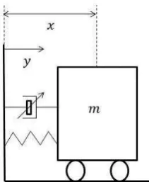
Initially, a base-excited SDOF system with nonlinear damping was considered (Figure 1). The equation of motion of the system is
(14)
where is a user-defined base acceleration, is the resulting displacement of the mass, is the damping ratio, is the natural frequency and modulates the level of Coulomb damping in the system. The magnitude of these parameters is shown in Table 1.
For the first part of this investigation, was chosen such that a square-wave base acceleration of amplitude 4 was used to excite the system:
(15)
The frequency of the square wave was left to be determined such that, in the context of this paper, . Each simulation of a real test was corrupted with Gaussian measurement noise of standard deviation
[image:4.595.382.488.523.652.2]which, depending on the excitation frequency, resulted in a signal-to-noise ratio of between 15 and 60.
Table 1: Parameters of the dynamical system described by equation (14).
Parameter Magnitude Units
0.01 -
rad/s N/kg
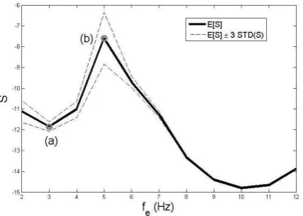
[image:5.595.60.274.235.387.2]Treating all of the model parameters ( ) as unknown, the entropy of the posterior parameter distribution was estimated for a range of different excitation frequencies. The ensemble average entropy, as well as confidence bounds, is shown in Figure 2.
Figure 2: Variation of the Shannon entropy with the frequency of a square-wave excitation for the system
described by equation (14).
It is immediately obvious that the entropy of the posterior will be minimised if one excites the system at its resonance frequency (10 Hz). This is simply because this maximises the signal-to-noise ratio – the relatively large response of the system is as far from the noise floor of the measurement noise as possible. It is important to note that Figure 2 shows the entropy of the entire posterior distribution – it does not show
how one’s confidence in each individual parameter estimate changes with (this is addressed in section 4.3 of the current work).
Two other points are of particular interest ((a) and (b) on Figure 2). According to the entropy estimates, point (b) (a square-wave excitation of 5 Hz) should yield relatively uncertain parameter estimates relative to point (a) (a square-wave excitation of 3 Hz). This was confirmed using MCMC simulations (the Metropolis algorithm specifically), the results of which are shown in Figure 3. The MCMC results have been normalised such that the Gaussian approximations of the posterior, which form an essential part of the entropy estimation, can be shown alongside. One can see that excitation (a) has indeed led to less uncertain parameter estimates relative to excitation (b). It is interesting to note that the Gaussian approximations are fairly poor, although they have still been able to predict which excitations will lead to better parameter estimates – this is a trend which the authors encountered throughout all the subsequent investigations.
Figure 3: MCMC results (black lines) and Gaussian approximations of the posterior distribution (grey lines) for the parameters of the system shown in equation (14). Plots (a)
and (b) refer to the excitations (a) and (b) on Figure 2.
SDOF System: Coulomb Nonlinearity with Sinusoidal 4.2
Excitation
In this section the natural frequency and damping ratio of the system was treated as known such that the magnitude of Coulomb damping was the only parameter to be found. Additionally, a sinusoidal excitation at the resonance frequency of the system was employed:
(15)
where the amplitude ( ) was left as a parameter to optimise. The resulting entropy estimates, as a function of , are shown in Figure 4. It is clear that, as one would expect, low amplitude excitations (such as point (a) on Figure 4) are beneficial when attempting to identify Coulomb-type nonlinearities. However it is also important to observe that, in the low amplitude regions, the response of the system is heavily corrupted by measurement noise – this has greatly increased the variance of the entropy estimates. It is also interesting to note that, above the amplitude indicated by point (b), the entropy is relatively unaffected by the amplitude of the excitation. This may be because the system is dominated by the linear response.
Figure 4: Variation of the Shannon entropy with the frequency of a sine-wave excitation for the system described
in equation (14).
SDOF System: Coulomb and Duffing-type 4.3
Nonlinearities and Sinusoidal Excitation
In this example a hardening Duffing-type spring was added to the system such that its equation of motion was now:
(15)
where controls the magnitude of the nonlinear spring. Throughout the following analysis, was set equal to
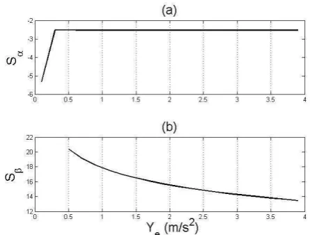
. Once again, a sinusoidal excitation was employed at a frequency of 10 Hz (and whose amplitude was to be optimised). The natural frequency and damping ratio of the system were considered known such that the parameters to be identified were and .
In this case, rather than tracking the entropy of the entire posterior distribution, it was assumed that and were uncorrelated such that
(16)
This allowed the entropy of the individual elements of the posterior (denoted and ) to be tracked separately (Figure 5). As with the previous example, the entropy of
is lowest for low excitations but, above a certain level, is relatively insensitive to the excitation amplitude. As one would expect, the entropy appears to be a strictly decreasing function of the excitation amplitude. The entropy of at lower levels of excitation is not shown on Figure 5 as, because of the large amounts of uncertainty involved, numerical overflow issues were encountered.
Figure 5: Variation of the Shannon entropy with the frequency of a sine-wave excitation for the system described
in equation (15).
Figure 5 presents an interesting conclusion. It suggests that, if one is wishing to simultaneously identify a Coulomb and Duffing-type nonlinearity using this type of excitation and can be considered a reasonable level of uncertainty with regard to the Coulomb damping estimate, then a large amplitude excitation is preferable. This is because the confidence one has in the magnitude of is insensitive to the excitation amplitude and so, therefore, one should simply choose the excitation which maximises one’s confidence in .
To validate this conclusion two sets of training data were created using excitation amplitudes of and respectively. MCMC simulations were then used to generate samples from the resulting posterior distributions. Figure 6 confirms that the use of a higher amplitude excitation
has greatly increased one’s confidence in the value of , while
it has had relatively little influence on one’s confidence in the
value of .
Figure 6: MCMC samples from the posterior shown in equation (16) where training data was generated using an amplitude of (a) 1 and (b) 4 . Dashed black lines
[image:6.595.65.281.76.245.2] [image:6.595.325.542.523.691.2]5 DISCUSSION AND FUTURE WORK
The authors intend to extend the preliminary study detailed in this paper in a variety of ways. For example, much of the analysis relies on the assumption that one already has a reasonable estimate of the optimum parameter vector . This may seem to be a somewhat circular argument as the overall aim of the proposed methodology is to design an experiment which allows one to obtain accurate estimates of . However, the ultimate goal of this work is to provide much more generic results. For example, in the case where one wishes to infer whether there is a combination of Coulomb and Duffing-type nonlinearities (of any magnitude) present in a system, it is hoped that the type of analysis detailed in this paper will be able to generate statements such as ‘a large amplitude excitation at the resonance frequency of the structure is required to test for these nonlinearities’. Additionally, the authors wish to extend the method such that it can aid in selecting the bandwidth of random excitations or the frequency and phase of multi-sine excitations.
Studying Figure 6, it is clear that the most probable parameters predicted by the MCMC simulations are biased. This highlights that, through using the method outlined in this paper, one defines the optimum excitation as being that which minimises parameter uncertainty (rather than that which minimises the bias in the most-probable parameter estimates). It would be interesting to see if, in future work, the phrase
‘optimum excitation’ can be defined as that which produces parameter estimates whose bias, as well as uncertainty, has been minimised.
Ultimately, before this work can be pursued further, the aim is to investigate how the proposed methodology can aid the system identification of real, laboratory-based systems.
6 CONCLUSIONS
Broadly speaking, this paper is concerned with the Bayesian system identification of dynamical systems using experimentally-obtained training data. An investigation is performed to find the optimum form of excitation that should be used during the generation of training data. This is achieved by using the Shannon entropy as an information measure such that, by estimating the entropy of the posterior parameter distribution, the information content of different sets of training data can be analysed. Using a series of simulations it is shown that such an approach can allow one to design experiments which, ultimately, will result in parameter estimates with minimal uncertainty.
REFERENCES
[1] Metropolis, N., Rosenbluth, A. W., Rosenbluth, M. N., Teller, A. H., & Teller, E. (1953). Equation of state calculations by fast computing machines. The journal of chemical physics, 21, 1087.
[2] Duane, S., Kennedy, A. D., Pendleton, B. J., & Roweth, D. (1987). Hybrid monte carlo. Physics letters B, 195(2), 216-222.
[3] Hukushima, K., & Nemoto, K. (1996). Exchange Monte Carlo method and application to spin glass simulations. Journal of the Physical Society of Japan, 65(6), 1604-1608.
[4] Marinari, E., & Parisi, G. (1992). Simulated tempering: a new Monte Carlo scheme. EPL (Europhysics Letters), 19(6), 451.
[5] Ching, J., & Chen, Y. C. (2007). Transitional Markov chain Monte Carlo method for Bayesian model updating, model class selection, and model averaging. Journal of engineering mechanics, 133(7), 816-832. [6] Green, P. J. (1995). Reversible jump Markov chain Monte Carlo
computation and Bayesian model determination. Biometrika, 82(4), 711-732.
[7] Green, P. L. (2014). Bayesian system identification of MDOF nonlinear systems using highly informative training data. Proceedings of IMAC XXXII, conference and exposition on structural dynamics – Orlando, Florida, 3-6 February 2014.
[8] Green, P.L. (2014). Bayesian system identification of dynamical systems using highly informative training data. Mechanical systems and signal processing (under review).