A model for cosmological
simulations of galaxy formation
physics: multi-epoch validation
The Harvard community has made this
article openly available.
Please share
how
this access benefits you. Your story matters
Citation
Torrey, Paul, Mark Vogelsberger, Shy Genel, Debora Sijacki, Volker
Springel, and Lars Hernquist. 2014. “A Model for Cosmological
Simulations of Galaxy Formation Physics: Multi-Epoch Validation.”
Monthly Notices of the Royal Astronomical Society 438 (3): 1985–
2004. https://doi.org/10.1093/mnras/stt2295.
Citable link
http://nrs.harvard.edu/urn-3:HUL.InstRepos:41381741
Terms of Use
This article was downloaded from Harvard University’s DASH
repository, and is made available under the terms and conditions
applicable to Open Access Policy Articles, as set forth at
http://
A physical model for cosmological simulations of galaxy
formation: multi-epoch validation
Paul Torrey
1?, Mark Vogelsberger
1†
, Shy Genel
1, Debora Sijacki
2, Volker Springel
3,4and Lars Hernquist
11 Harvard-Smithsonian Center for Astrophysics, 60 Garden Street, Cambridge, MA, 02138, USA
2 Institute of Astronomy and Kavli Institute for Cosmology, University of Cambridge, Madingley Road, Cambridge CB3 0HA 3 Heidelberg Institute for Theoretical Studies, Schloss-Wolfsbrunnenweg 35, 69118 Heidelberg, Germany
4 Zentrum f¨ur Astronomie der Universit¨at Heidelberg, ARI, M¨onchhofstr. 12-14, 69120 Heidelberg, Germany
5 August 2018
ABSTRACT
We present a multi-epoch analysis of the galaxy populations formed within the cos-mological hydrodynamical simulations presented in Vogelsberger et al. (2013). These simulations explore the performance of a recently implemented feedback model which includes primordial and metal line radiative cooling with self-shielding corrections; stellar evolution with associated mass loss and chemical enrichment; feedback by stel-lar winds; black hole seeding, growth and merging; and AGN quasar- and radio-mode heating with a phenomenological prescription for AGN electro-magnetic feedback. We illustrate the impact of the model parameter choices on the resulting simulated galaxy population properties at high and intermediate redshifts. We demonstrate that our scheme is capable of producing galaxy populations that broadly reproduce the ob-served galaxy stellar mass function extending from redshift z = 0 toz = 3. We also characterise the evolving galactic B-band luminosity function, stellar mass to halo mass ratio, star formation main sequence, Tully-Fisher relation, and gas-phase mass-metallicity relation and confront them against recent observational estimates. This detailed comparison allows us to validate elements of our feedback model, while also identifying areas of tension that will be addressed in future work.
Key words: methods: numerical – cosmology: theory – cosmology: galaxy formation
1 INTRODUCTION
Cosmological simulations are among the most powerful tools available for studying the non-linear regime of cosmic struc-ture formation. While dark matter only simulations have built a solid foundation for our understanding of the origin of haloes via gravitational collapse (e.g., Springel et al. 2005c; Boylan-Kolchin et al. 2009; Fosalba et al. 2008; Teyssier et al. 2009; Klypin et al. 2011), applying their findings to our understanding of the observable Universe (i.e. luminous galaxies) requires modelling of baryonic physics as well. Al-though semi-analytic (e.g., White & Frenk 1991; Kauffmann et al. 1999; Hatton et al. 2003; Kang et al. 2005; Somerville et al. 2008; Guo et al. 2011, 2012) and halo occupation dis-tribution (e.g., Vale & Ostriker 2004; Conroy et al. 2006;
? E-mail: [email protected]
† Hubble Fellow.
Behroozi et al. 2012; Moster et al. 2012) models can esti-mate galaxy properties based on dark matter only simula-tions, the most direct and self-consistent way to explore the evolution of observable galaxies theoretically is by including baryons in the simulations (e.g. Katz et al. 1992, 1996; Wein-berg et al. 1997; Murali et al. 2002; Springel & Hernquist
2003b; Kereˇs et al. 2005; Ocvirk et al. 2008; Crain et al.
2009; Croft et al. 2009; Schaye et al. 2010; Oppenheimer et al. 2010; Vogelsberger et al. 2012).
The main challenge for any large-scale galaxy forma-tion model is accurately handling the baryonic physics and including proper forms of feedback to regulate star forma-tion. Galaxy formation simulations lacking strong feedback substantially overproduce stars, leading to galaxies with too high baryon fractions (e.g., White & Frenk 1991; Balogh et al. 2001; Scannapieco et al. 2012). This problem is most pronounced for the highest and lowest mass systems, where star formation is known to be relatively inefficient (e.g.,
Behroozi et al. 2012, and references therein). The problem can be remedied by introducing sources of feedback which ei-ther eject gas from galaxies or heat it to prevent continued accretion from the halo. Two commonly employed strong feedback mechanisms are star formation (Dekel & Silk 1986; Thacker & Couchman 2000; Springel & Hernquist 2003a; Kawata & Gibson 2003; Stinson et al. 2006; Scannapieco et al. 2008; Dalla Vecchia & Schaye 2008; Okamoto et al. 2010; Stinson et al. 2013) and black hole growth (Springel et al. 2005b; Kawata & Gibson 2005; Di Matteo et al. 2005; Thacker et al. 2006; Sijacki et al. 2007; Okamoto et al. 2008; Kurosawa & Proga 2009; Booth & Schaye 2009; Debuhr et al. 2011; Dubois et al. 2012).
Winds driven by star formation are a consequence of en-ergy and/or momentum injection from newly formed stellar populations into the interstellar medium (ISM). Observa-tions indicate that star forming galaxies show signs of out-flowing material (e.g., Heckman et al. 2000; Rupke et al. 2002, 2005), and that the velocity of the outflowing wind ma-terial may scale with the mass of the galaxy (Martin 2005). Including winds in large-scale cosmological simulations re-quires sub-grid models because the detailed ISM structure remains unresolved (Hopkins et al. 2012a, 2013a,b). Several types of explicit wind models have been developed including hydrodynamically decoupled winds (Springel & Hernquist 2003a), injecting thermal energy while shutting down cool-ing (Stinson et al. 2006, 2013), or addcool-ing blast particles to launch a Sedov-Taylor blast wave (Dubois & Teyssier 2008). These wind prescriptions vary in their formulations, but all of them eject material from galaxies based on the local star formation rate and they have all been shown capable of reg-ulating the growth of low mass galaxies in large scale
simu-lations (e.g., Dav´e et al. 2011b; Kannan et al. 2013; Ocvirk
et al. 2008).
Feedback from active galactic nuclei (AGN) is the re-sult of energy and/or momentum injection that occurs as gas accretes onto the galaxy’s central super-massive black hole (BH). This is thought to be responsible for the rapidly-moving outflows that can be inferred from UV and X-ray observations of galaxies that host AGN (Chartas et al. 2002; Pounds et al. 2003; Reeves et al. 2003). It has been shown that AGN feedback is critical for heating gas in deep grav-itational potentials (e.g., Sijacki & Springel 2006), shutting down star formation (e.g., Springel et al. 2005b,a; Croton et al. 2006; Hopkins et al. 2006; Sijacki et al. 2007; Hopkins et al. 2008a; Booth & Schaye 2009; McCarthy et al. 2010), and setting up self-regulated black hole growth (Di Matteo et al. 2005; Hopkins et al. 2006, 2007a,b, 2008b; Di Matteo et al. 2008; Younger et al. 2008; Sijacki et al. 2009).
Over the last few years, there have been many studies of galaxy formation using large-scale hydrodynamical simula-tions. For example, Schaye et al. (2010) presented a suite of smoothed particle hydrodynamics (SPH) simulations (the “OWLS” project) to explore the impact of various physi-cal effects, like stellar and AGN feedback, on the resulting galaxy population. The simulations were used to examine, among other things, the evolution of the cosmic star forma-tion rate (Schaye et al. 2010), observaforma-tional signatures of the warm-hot intergalactic medium (Tepper-Garc´ıa et al. 2011, 2012), and the rates and modes of gas accretion into dark matter haloes (van de Voort et al. 2011; van de Voort &
Schaye 2012; van de Voort et al. 2012). More recently, Dav´e
et al. (2011b) used SPH simulations to investigate the im-pact and importance of stellar winds. They found that stellar
winds are able to reproduce the faint-end of thez= 0 galaxy
stellar mass function, while also leading to appropriate levels of enrichment in the inter galactic medium (Oppenheimer &
Dav´e 2008; Oppenheimer et al. 2009). Even more recently,
it was shown (Kannan et al. 2013) that large-scale hydrody-namical simulations are capable of producing galaxy stellar mass functions and stellar mass to halo mass relations that are consistent with observations by enforcing strong (Stinson et al. 2006) and early (Stinson et al. 2013) stellar feedback. In the “GIMIC” project (Crain et al. 2009), roughly
spherical volumes of size L ∼ 20h−1 Mpc drawn from
re-gions of various over-densities in the Millennium simula-tion were re-simulated at high resolusimula-tion. This work has been used to study systematic variations in galaxy formation that scales with large scale environment (Crain et al. 2009), the formation (Font et al. 2011) and structure (McCarthy et al. 2012a) of galactic stellar haloes, and the characteris-tics (McCarthy et al. 2012b) and origin (Sales et al. 2012) of disk galaxies. The “Mare-Nostrum Horizon” (Ocvirk et al. 2008) is perhaps the largest, high-resolution, full-volume cos-mological simulation run and it was performed using the
Adaptive Mesh Refinement (AMR) simulation code
RAM-SES(Teyssier 2002). This simulation was used to study the
mode of gas accretion into galaxies (Ocvirk et al. 2008) and the angular momentum evolution of high redshift galax-ies (Danovich et al. 2012). Other simulations aimed at study-ing galaxy formation in large volumes have been carried out
usingRAMSESby Hahn et al. (2010) and Few et al. (2012).
Recently, a moving-mesh hydro solver was developed and incorporated into the hydrodynamical simulation code
AREPO(Springel 2010). This method combines advantages of traditional Lagrangian hydro solvers (e.g., continuous res-olution enhancement, adaptive geometry, Galilean invari-ance) with the strengths of Eulerian hydro solvers (e.g., in-stability handling, shock capturing, phase boundary resolu-tion). It has been demonstrated that the hydro solver used inAREPOcan lead to systematic changes in the properties of galaxies formed in cosmological simulations. In particu-lar, the hot-haloes of galaxies are found to contain less hot gas (Vogelsberger et al. 2012) because it is able to cool
effi-ciently onto the central gas disk (Sijacki et al. 2012; Kereˇs
et al. 2012). This leads to an increase in hot-mode gas ac-cretion rates (Nelson et al. 2013) and the creation of large, gas disks (Torrey et al. 2012). However, the first cosmologi-cal simulations published with this code lacked strong feed-back, and therefore formed stars far too efficiently compared to actual galaxies.
The goal of this paper is to test and demonstrate the
ability of theAREPOcode to produce realistic galaxy
popu-lations directly in cosmological simupopu-lations by including re-alistic feedback processes. This paper builds on the work pre-sented in Vogelsberger et al. (2013, hereafter, Paper I) where a detailed description of our galaxy formation model for the
moving mesh codeAREPOwas presented for the first time.
In Paper I, the framework of our approach was described in detail and a set of cosmological simulations were presented. The strength of the star formation driven winds and the AGN feedback parameters were tuned as to accurately re-produce the evolving cosmic star formation rate density and
content of ejected wind material was set to ensure a
rea-sonable normalization of the redshiftz= 0 mass-metallicity
relation. These relations, as well as several other redshift
z = 0 relations that were not used to tune the feedback
model (e.g., the Tully-Fisher relation and luminosity func-tions) were presented in Paper I. The primary goal in what follows is to extend the analysis of Paper I by benchmark-ing the performance of our galaxy formation models against observational constraints at intermediate and high redshifts. This allows us to understand if the simulated galaxy popula-tions are forming and evolving in a manner consistent with observations.
The structure of this paper is as follows: In Section 2 we describe the simulations that we have used, including a brief description of our general methods and the various feedback mechanisms included in our simulations. We present results of the build-up of stellar mass in Section 3, the evolution of the galactic and global star formation rates in Section 4, and the evolution of the mass-metallicity relation and Tully-Fisher relation in Section 5. We discuss our results and conclude in Section 6.
2 METHODS
The simulation suite used in this paper as well as a detailed description of our numerical methods have been discussed extensively in Paper I. We review briefly the main compo-nents of the galaxy formation model here.
All simulations used in this paper, apart from the ‘no-feedback’ run, include the same physics: gravity, hydrody-namics, radiative gas cooling, star formation with associated feedback, and AGN feedback. The gravity and hydrodynam-ics implementation are described in Springel (2010) and Vo-gelsberger et al. (2012). Radiative gas cooling for hydrogen and helium is carried out according to Katz et al. (1996) taking into account the presence of a cosmologically evolving
ultraviolet background (Faucher-Gigu`ere et al. 2009), which
has been calibrated to match the mean transmission of the
Lyman-alpha forest at redshiftsz= 2−4.2 (Faucher-Gigu`ere
et al. 2008b,a), HeII reionisation byz∼3 (McQuinn et al.
2009), and complete HI reionisation byz = 6. In addition,
the metal line contribution to the cooling rate is tabulated as a function of gas density, temperature, redshift-dependent background radiation, and metallicity using the
photoioni-sation codeCLOUDY(Ferland et al. 1998, 2013) and added
to the primordial cooling rate. We correct both cooling con-tributions for self-shielding (Rahmati et al. 2013).
Star formation is modelled using a slightly modified version of the Springel & Hernquist (2003a) subgrid model which pressurises gas above the specified star formation sity threshold and converts gas into stars according to a den-sity based prescription that is tuned to recover the observed Kennicutt-Schmitt (Kennicutt 1998; Schmidt 1959) relation for star forming gas. The equation of state parameter used is
qeos= 0.3, which allows for resolution of internal disk
struc-tures yet prevents artificial gas fragmentation (Springel et al. 2005b; Robertson et al. 2006) and is also consistent with a value derived in the high-resolution ISM simulations of Hop-kins et al. (2012b).
Stellar mass loss and metal enrichment are carried out by calculating the mass and composition of ejected material
from aging stellar populations at each time-step. To achieve this, we adopt a Chabrier (2003) initial mass function (IMF), the stellar lifetime function from Portinari et al. (1998), and the chemical yields for asymptotic giant branch (AGB) stars (Karakas 2010), core collapse supernovae (Portinari et al. 1998), and Type Ia supernovae (Thielemann et al. 1986). The star formation driven wind model uses a stochas-tic approach, similar to Springel & Hernquist (2003a), to launch wind particles out of star forming regions. We adopt a variable wind speed that drives winds at a velocity based on the local dark matter velocity dispersion (e.g.,
Oppen-heimer & Dav´e 2006, 2008). The mass loading factor is
ad-justed appropriately based on the local velocity dispersion such that an equal amount of energy is transferred to the ISM per unit star formation rate (SFR) (Okamoto et al.
2010). We have introduced a wind metal loading factor,γw,
which is set independently from the wind mass loading
fac-tor,ηw. The wind metal loading factor defines the
relation-ship between the metallicity of newly created wind particles,
Zw, and the metallicity of the ambient ISM,ZISM, such that
Zwind=γZISM. We adopt a metal loading factor ofγw= 0.4
which allows for reasonable matches to the local and high redshift mass-metallicity relation, halo gas enrichment, and galaxy gas-phase metallicity gradients.
We adopt a unified model for quasar (Springel et al. 2005b; Di Matteo et al. 2005, 2008), radio (Sijacki et al. 2007), and radiative AGN feedback. The quasar mode self-regulates the black hole growth by injecting thermal energy around the black hole at a rate proportional to the black hole accretion rate. For lower accretion rates (in Edding-ton units), off-center radio-mode bubbles are generated. The AGN radiative feedback prescription provides a novel way for black holes to impact the gas state at large distances by suppressing gas cooling. While the majority of the gas in our cosmological box cools under the assumption of being exposed to a uniform UV background, the cooling rate of gas near BHs is calculated from a combination of both the uniform UV background and the ionising radiation field of nearby AGN.
All of the simulations in this paper were performed in
periodic boxes of size L = 25h−1Mpc. The number of dark
matter elements remains constant throughout the simula-tion with a particle mass dependent on the simulasimula-tion res-olution as noted in Table 1. The mass within individual resolution elements for the gas changes as material is ad-vected across cell boundaries and the number of gas elements changes as cells can be converted into collisionless stellar particles and accreted by black holes. However, we include a cell (de-)refinement scheme (Vogelsberger et al. 2012) which enforces that all cells remain within a factor of two of a specified target mass so that the total number of baryonic elements in our simulations (star particles and gas cells) re-mains close to its initial value. All simulations use initial
conditions generated at redshiftz= 127 based on a CAMB
linear power spectrum. The adopted cosmological
parame-ters are Ωm0 = 0.27, ΩΛ0= 0.73, Ωb0 = 0.0456, σ8 = 0.81,
and H0 = 100hkm s−1Mpc−1 = 70.4 km s−1Mpc−1 (h =
0.704), which are consistent with Komatsu et al. (2011).
We study two types of simulations in this paper, both of which were described in Paper I. The first is a set of
cos-mological simulations of size L = 25h−1Mpc that initially
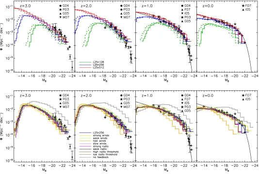
Figure 1.The simulated galaxy stellar mass function (GSMF) is shown for three different resolution simulations (top panel, solid coloured lines) and several variations of our feedback model (bottom panel, solid coloured lines) along with data points from observations at four different redshifts (as indicated). The “no feedback” simulation (grey line, bottom plot) provides a poor match to observations, underscoring the need for strong feedback to regulate the growth of galaxies. Many of the feedback models are able to alleviate the overproduction of stellar mass, including the high resolution fiducial model (red line, top plot) which provides reasonable agreement in the overall shape and normalisation of the GSMF compared against observations. This includes a flattening of the low mass end of the GSMF that occurs towards late times, along with a sharp cutoff for massive systems.
we vary the parameter choices for our feedback model. The impact of these feedback parameter variations on the
red-shiftz= 0 galaxy population was discussed in Paper I, and
we extend this discussion here by comparing the simulated galaxy populations with high redshift data. The second set of simulations employs our fiducial feedback model at three dif-ferent resolutions, and are labelled L25n128, L25n256, and L25n512. All our simulations are summarised in Table 1.
We use theSUBFINDalgorithm (Springel et al. 2001) to
identify gravitationally bound groups of dark matter, stars, and gas. We treat each self-bound group as a galaxy, and
calculate its properties based on the SUBFIND (sub) halo
catalogue. For the stellar mass, we could in principle take a sum over all stellar particles associated with the group. However, a non-negligible fraction of stellar mass in mas-sive systems resides in a diffusely distributed component, as seen in observations of groups and clusters (e.g., Zibetti et al. 2005; McGee & Balogh 2010) and simulations (e.g., Murante et al. 2004, 2007; Rudick et al. 2006; Puchwein
et al. 2010; Puchwein & Springel 2013). This is an impor-tant point because: (i) intra-cluster light is not traditionally counted as contributing to the central galaxy’s mass and (ii) some of the intra-cluster light may fall below observational limits. To take this into account, we define the galactic stel-lar mass as the sum of stelstel-lar mass within twice the (total) stellar half mass radius. This has only a small effect on the stellar mass measurements for low mass systems, but can reduce the intra-cluster mass contributions in more massive systems. We have checked that our adopted definition of galactic stellar mass gives a similar result compared to what would be obtained if we used an observationally motivated surface brightness cut for massive systems (e.g., Rudick et al.
2006). For the halo mass we adopt theM200,critvalue, which
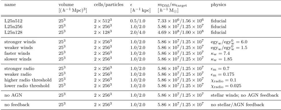
name volume cells/particles mDM/mtarget physics [(h−1Mpc)3] [h−1kpc] [h−1M
]
L25n512 253 2×5123 0.5/1.0 7.33×10⁶/1.56×106 fiducial
L25n256 253 2×2563 1.0/2.0 5.86×10⁷/1.25×107 fiducial
L25n128 253 2×1283 2.0/4.0 4.69×10⁸/1.00×108 fiducial
stronger winds 253 2×2563 1.0/2.0 5.86×10⁷/1.25×107 egy
w/egy0w= 6.0
weaker winds 253 2×2563 1.0/2.0 5.86×10⁷/1.25×107 egy
w/egy0w= 1.5
faster winds 253 2×2563 1.0/2.0 5.86×10⁷/1.25×107 κw= 7.4
slower winds 253 2×2563 1.0/2.0 5.86×10⁷/1.25×107 κw= 1.85
stronger radio 253 2×2563 1.0/2.0 5.86×10⁷/1.25×107 m= 0.7
weaker radio 253 2×2563 1.0/2.0 5.86×10⁷/1.25×107 m= 0.175
higher radio threshold 253 2×2563 1.0/2.0 5.86×10⁷/1.25×107 χradio= 0.1
lower radio threshold 253 2×2563 1.0/2.0 5.86×10⁷/1.25×107 χradio= 0.025
no AGN 253 2×2563 1.0/2.0 5.86×10⁷/1.25×107 stellar winds; no AGN feedback
[image:6.612.48.535.70.261.2]no feedback 253 2×2563 1.0/2.0 5.86×10⁷/1.25×107 no stellar/AGN feedback
Table 1. Summary of the different cosmological simulations as originally described in Paper I, and as referenced throughout this paper. The L25n128, L25n256, L25n512 simulations employ the fiducial physics parameters shown in Table 1 of Paper I. The remaining simulations explore variations in our feedback model parameters at the intermediate resolution. Parameters that are varied are indicated in the last column.
3 THE STELLAR CONTENT OF GALAXIES
The shape of the galaxy stellar mass function (GSMF) is de-termined by a combination of the underlying DM (sub)halo mass function (HMF), and the efficiency with which stars are formed in those haloes. As noted previously, including winds driven by star formation is critical to reproducing the evolving number density of low mass galaxies (Oppenheimer et al. 2010; Bower et al. 2012; Puchwein & Springel 2013) while AGN feedback can quench star formation in massive haloes, establishing a high mass cutoff in the GSMF (Cro-ton et al. 2006; Hopkins et al. 2008a; Gabor et al. 2011; Bower et al. 2012; Puchwein & Springel 2013). Both of these feedback processes have been included in our simulations as described in the previous section, and as has already been shown in Paper I the model included in our simulations is capable of producing reasonable matches to the GSMF at
redshiftz= 0. In this section, we focus on the evolution of
the GSMF with time, and compare the simulation results with several recent observations (summarised in Table 2). We have applied appropriate correction factors to all obser-vational stellar mass measurements so that all results are now appropriate for a Chabrier (2003) initial mass function (IMF).
A comparison of the simulated GSMF with observa-tions is presented in Figure 1. The bottom panel of Figure 1 shows the simulated GSMF for several variations of our feed-back model. Most of the feedfeed-back models provide
satisfac-tory fits to the redshiftz= 3 GSMF. The one exception is
the “strong winds” simulation, which suppresses the stellar mass growth of galaxies slightly too efficiently, and lowers
the normalisation of the simulated GSMF. By redshiftz= 2
the offset of the strong wind model is less distinct, and all of the feedback runs provide good fits to the observational data, especially compared to the “no feedback” case. At
red-shiftz= 1 most of the feedback models deviate from
obser-vations in the normalisation of the GSMF at the low mass end. This is an indication that low mass systems in our
sim-ulations are building up their stellar mass at this epoch more efficiently than observations indicate. The exception is the “fast wind” model, which produces a GSMF that is offset to-ward lower normalisations (compared to the other feedback
models), consistent with observations. By redshift z = 0,
this normalisation offset is reduced for most of the feedback models, as the observed number density of low mass sys-tems has substantially increased, while the number density of these same objects has remained fairly constant in the simulations. While the “fast wind” simulation provided the
best fit to the GSMF at redshiftz= 1, this same simulation
now strongly underproduces galaxies just below the knee of the GSMF.
Our simulation shows an appropriate exponential cut-off in the GSMF at low redshift for massive galaxies. The simulation box used here is too small to identify this expo-nential cutoff clearly at early redshifts. Where it is seen, the exponential drop is driven by efficient AGN radio-mode feed-back in our simulations which suppresses star formation in massive systems (Croton et al. 2006; Hopkins et al. 2008a; Guo et al. 2010; Bower et al. 2012; Puchwein & Springel 2013). The exact location of this cutoff depends on choices for the AGN radio feedback strength and accretion thresh-old, as discussed in Paper I. Obtaining this cutoff is impor-tant because it indicates that all haloes will have reason-ably sized stellar components associated with them. This allows for a clear connection between the properties (i.e. the growth rates, concentrations, morphologies, etc.) of observ-able galaxies and their host dark matter haloes.
The resolution dependence of the simulated GSMF is shown for the fiducial feedback model in the top panel of Figure 1. We note three points regarding the numerical con-vergence of the simulated GSMF. First, any resolution ef-fects become increasingly prominent toward late times. Al-though all three resolution simulations agree fairly well at
redshiftz = 3, the redshift z = 0 agreement is less good.
Second, while there is an offset between the normalisations
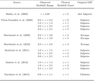
Table 2.Observational references for the galaxy stellar mass function data used in Figure 1.
Source Observed Plotted Original IMF Redshift Range Redshift Panel
Baldry et al. (2008) z <0.05 z= 0 diet Salpeter
P´erez-Gonz´alez et al. (2008) 0.0< z <0.2 z= 0 Salpeter 1.0< z <1.3 z= 1 Salpeter 2.0< z <2.5 z= 2 Salpeter 3.0< z <2.5 z= 3 Salpeter
Marchesini et al. (2009) 2.0< z <3.0 z= 2 Kroupa 3.0< z <4.0 z= 3 Kroupa
Marchesini et al. (2010) 3.0< z <4.0 z= 3 Kroupa
Mortlock et al. (2011) 1.0< z <1.5 z= 1 Salpeter 2.0< z <2.5 z= 2 Salpeter 3.0< z <3.5 z= 3 Salpeter
Santini et al. (2012) 1.0< z <1.4 z= 1 Salpeter 1.8< z <2.5 z= 2 Salpeter 2.5< z <3.5 z= 3 Salpeter
Davidzon et al. (2013) 0.9< z <1.1 z= 1 Chabrier
resolution simulation GSMFs which is visible at late times,
the offset between the intermediate (2563) and high (5123)
resolution simulations GSMFs is smaller. This indicates that our results are converging numerically. Third, the GSMF for
high mass systems (e.g.,M∗>1010M) shows little offset
at any redshift for the two highest resolution simulations, which indicates these systems are numerically converged. In fact, it is likely that the GSMF is converged down to even
lower masses (e.g.,M∗>109M) for our highest resolution
simulations. However, we could only demonstrate this point by presenting an even higher resolution simulation, which is beyond the scope of this paper.
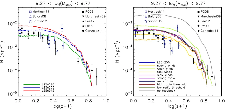
A clear characterisation of the performance of our var-ious feedback models can be obtained by independently as-sessing the evolution of the slope and normalisation of the low mass end of the GSMF. As mentioned above, the major-ity of our feedback models appear to overproduce the
num-ber density of low mass galaxies at redshiftz= 1. The right
panel of Figure 2 highlights this by showing the number den-sity evolution of simulated low mass galaxies (in the same particular mass bin used in Weinmann et al. 2012). Wein-mann et al. (2012) argued that the shape of the low mass galaxy number density evolution in previous semi-analytic and hydrodynamical modeling is characteristically distinct from that of the observations, indicating that the models were not using wind prescriptions capable of decoupling the galaxy stellar mass growth from the underlying halo mass growth. Here, we find that all of our feedback choices lead to a very flat evolution in the number density of these low mass
systems past redshiftz= 1. Variations in our adopted wind
model set the normalisation of the low redshift number den-sity plateau, but do not strongly impact the slope. Whereas the “weak winds” model leads to a higher number density of
low mass systems, the “strong winds” model decreases the number density of low mass systems. Since all of our mod-els plateau in their low mass number density at late times while the observations indicate an increasing number den-sity of these systems, it is unlikely that any simple variation in our wind model could reproduce the observed redshift
z= 1 andz= 0 low mass galaxy number densities
simulta-neously. It is worth noting here that, as expected, variations in the adopted black hole feedback model parameters have negligible impact on the evolution of the simulated low mass galaxy population.
The left panel of Figure 2 demonstrates the resolution dependence of the number density evolution of low mass galaxies. All resolution simulations show the same character-istic evolutionary shape. Higher resolution simulations pro-duce slightly higher normalisations, due to increases in the star formation efficiency in low mass galaxies. The magni-tude of this resolution dependence decreases towards better resolved systems. The highest resolution model passes above most of the low redshift data points and misses the interme-diate redshift data points. This may be an indication that our models require more efficient suppression of star forma-tion in low mass systems at these redshifts. But, as discussed above, while simply tuning up the strength of our wind feed-back model could correct the normalisation of the low mass galaxy number density at either low or intermediate red-shifts, we cannot correct the normalisation at both epochs simultaneously.
Figure 2.The evolution of the number density of low mass galaxies is shown for three different resolutions (left) and our varied feedback models (right). The black symbols show the data taken directly from the Weinmann et al. (2012) paper, while the blue points show additional data points assembled by interpolating/extrapolating the GFMS data used in Figure 1 of this paper. As in many semi-analytic and hydrodynamic models, low mass systems are being assembled too early, leading to an overproduction of these systems by redshift
z∼1, with little evolution in their number density thereafter. Variations in the feedback parameters lead to adjusted normalisations for the late time number density plateau, without substantially impacting the late time slope.
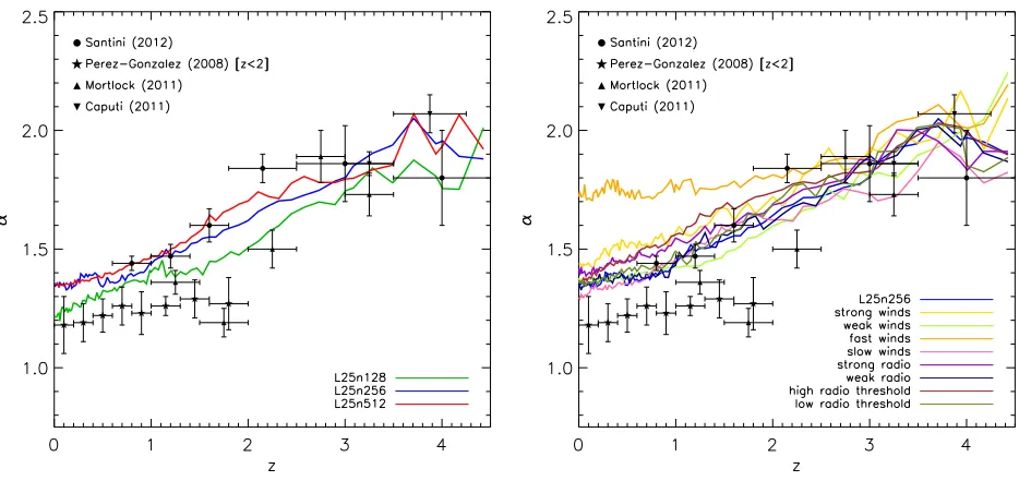
Figure 3 shows the low mass end slope,α, compared to
ob-servational results for the various feedback model
parame-terisations. Here we note that P´erez-Gonz´alez et al. (2008)
caution that their estimations of the low-mass end slope of
the GSMF above redshiftz&2 could be affected by
incom-pleteness. Thus, as indicated in the legend of Figure 3, we
have removed thez >2 slope calculations of P´erez-Gonz´alez
et al. (2008). Most of the simulations are clustered around a single evolutionary track that traces the observed low mass
end slope evolution. We do not show a best fitαvalue for the
“no feedback” simulation because the low redshift GSMF is not well described by a single Schechter function. The most substantially offset model is the “fast wind” model, which has a steeper slope than observations (see Figure 1 and dis-cussion above). All of the other feedback models produce evolving low mass end slopes which are similar to the obser-vations.
There is no major resolution dependence to this result, as demonstrated in the left panel of Figure 3. The fidu-cial feedback model yields very similar low mass end GSMF slopes for all three resolutions. In particular, the intermedi-ate and high resolution runs show very similar low redshift behaviour, indicative of numerical convergence.
3.1 Luminosity Function
Comparing our simulated GSMFs to observations implicitly assumes that the observed spectra can be converted into stellar mass measurements accurately. Stellar mass measure-ments are typically obtained from observations by employ-ing stellar population synthesis models (e.g., Leitherer et al. 1999; Bruzual & Charlot 2003; Le Borgne et al. 2004) and
assuming some star formation history and IMF. However, there are a number of uncertainties associated with observa-tionally determined stellar mass measurements, and so some caution should be taken when comparing to theoretically de-termined stellar mass measurements (Mitchell et al. 2013). Instead of considering the stellar mass function comparison of the previous subsection alone, it is useful to also consider how the luminosity functions compare between the simu-lations and observations. To facilitate this comparison, we assign broad band luminosities to all star particles in each galaxy via the Bruzual & Charlot (2003, hereafter BC03) catalogues after taking into account the star particle’s age, initial stellar mass, metallicity, and assuming a Chabrier (2003) IMF. To start, we neglect the impact of dust atten-uation, and tabulate each galaxy’s luminosity as the sum of the contributions from all of its star particles.
It was shown in Paper I that our galaxy formation model produces luminosity functions that agree with local SDSS g-, r-, i-, and z-band measurements. To extend the comparison of the observed and simulated results to higher redshift, we consider the rest-frame B-band luminosity func-tion versus redshift as shown in Figure 4. Observafunc-tional data points are included for comparison as outlined in Table 3. As in Figure 1, the top panel of Figure 4 shows the resolution dependence of the simulated redshift dependent luminosity function while the bottom panel shows the impact of the feedback model parameter choices on the simulated lumi-nosity function.
The luminosity function is impacted by feedback in a very similar way to the GSMF. Most of the feedback
mod-els provide satisfactory fits to the redshiftz = 3
Figure 3.The evolution of the low mass end slope of the galaxy stellar mass function is shown for three different resolutions (left) and our varied feedback models (right). We have obtained theαslope value by performing an RMS minimisation to determine the best fit Schechter function parameters. Observational estimates ofαfrom the literature are also shown.
is offset towards marginally brighter values. Since no
sub-stantial offset exists in the redshift z = 3 GSMF
simula-tion/observation comparison at the same number density, this may be an indication that our simulated systems need marginally higher star formation rates (i.e. have somewhat younger stellar populations) to better match the B-band luminosity function. This, however, may give rise to other tensions in either the global star formation rate density or star formation main sequence relations which we discuss in the next section. It is also possible that omitting non-stellar sources of luminosity (e.g., AGN) could be leading to an un-derestimation of simulated galaxies true B-band luminosi-ties.
At redshiftsz= 2 andz = 1 we find very good
agree-ment between the simulated and observed luminosity func-tions in terms of overall shape and normalisation for most of the feedback models. The two clear outlier simulations are the “no feedback” case (which allows for efficient star formation in all galaxies, making haloes/galaxies of a given number density too bright) and the “fast wind” case (which suppresses star formation in massive systems too efficiently, and therefore underproduces bright objects). As with the GSMF, the various model parameter choices for the AGN feedback have little impact here, because of the lack of very massive/bright objects in our small simulation volume. By
redshift z = 0, there is a broader spread in the
luminos-ity functions that result from the different models, with the best agreement to the observed B-band luminosity function being given by our fiducial “L25n256” model, as discussed in Paper I.
The resolution dependence of the simulated luminosity function is demonstrated for our fiducial feedback model in the top panel of Figure 4. There is a slight increase in the normalisation of the luminosity function for higher resolu-tion simularesolu-tions, however this normalisaresolu-tion offset is small
between the intermediate and high resolution cases. Overall, the similarity of the intermediate and high resolution sim-ulations indicates reasonable numerical convergence for our fiducial feedback model.
To this point, we have neglected the impact of dust at-tenuation which can have a substantial impact on the mea-sured B-band luminosity function (e.g., Tuffs et al. 2004; Pierini et al. 2005). We can approximate the dust attenua-tion correcattenua-tion to the simulated B-band luminosity funcattenua-tion using the simple model of Charlot & Fall (2000). The dust attenuated B-band luminosity functions from our models are shown in the top panel of Figure 4 as a series of
col-ored dashed lines. The size of the correction is∼0.5
mag-nitudes, and pushes our models away from the observations at all redshifts. This exacerbates the previously discussed shortfall of our models with respect to the bright end of the
luminosity function at redshift z = 3, and creates a
simi-lar issue at lower redshifts. However, the normalization and slope of the faint end of the luminosity function remains almost unchanged where our models continue to provide a good match to the observations. More detailed modeling of the dust attenuation will be considered in future work via three-dimensional radiative transfer to self-consistently de-termine line-of-sight attenuation factors under more explicit assumptions (e.g., the dust-to-gas ratio) which may validate or correct the luminosity functions presented here.
In general, the simulated luminosity functions agree well
with observations up to redshiftz= 3. Perhaps this is
Table 3. Observational references for the luminosity function data used in Figure 4.
Source Observed Plotted Redshift Ranges Redshift Panel
Poli et al. (2003) 0.7< z <1.0 z= 1 1.3< z <2.5 z= 2 2.5< z <3.5 z= 3
Gabasch et al. (2004) 0.8< z <1.2 z= 1 1.75< z <2.5 z= 2 2.5< z <3.4 z= 3
Giallongo et al. (2005) 0.7< z <1.0 z= 1 1.3< z <2.5 z= 2 2.5< z <3.5 z= 3
Ilbert et al. (2005) 0.05< z <0.2 z= 0 1.0< z <1.3 z= 1
Faber et al. (2007) 0.2< z <0.4 z= 0 1.0< z <1.2 z= 1
Marchesini et al. (2007) 2.0< z <2.5 z= 2 2.5< z <3.5 z= 3
accounting for the finite recycling time for previously ejected wind material (Henriques et al. 2012) as is done in our
sim-ulations (see discussion in Oppenheimer & Dav´e 2008, for
more details on the recycling time for wind material). The two most obvious ways that we could have achieved agree-ment in the stellar mass functions without obtaining similar agreement in the luminosity functions is by forming galaxies in our simulation with very different star formation histo-ries from that assumed by observational models, or, if our assumption of neglecting dust attenuation failed severely. It is unlikely that we have formed galaxy populations with very different formation histories because, as we will show in the next section, the simulated global SFR as well as the simulated star formation main sequence both follow obser-vations reasonably well. While we have not carried out a full radiative transfer calculation to determine the impact of dust attenuation, we have shown that our fiducial models only slightly undershoot the observational measurements of the B-band luminosity function when we approximate dust attenuation via the simple model of Charlot & Fall (2000).
3.2 Stellar Mass vs. Halo Mass
Within the past decade, abundance matching models have brought together measurements of the galaxy stellar mass functions with detailed numerical models of structure forma-tion (Conroy et al. 2006; Conroy & Wechsler 2009; Moster et al. 2010; Guo et al. 2010; Moster et al. 2012; Behroozi et al. 2012). By relying on a simple central assumption to pair the population of simulated dark matter haloes to ob-served galaxies (e.g., based on mass), a more detailed link between observed galaxies and their host dark matter haloes has been established along with an understanding of how
galaxies and their host haloes evolve together in time. In particular, one of the central results from these models is a parameterised relationship describing the evolution of the stellar mass to halo mass (SMHM) ratio as a function of galaxy mass and redshift. Comparing directly to abundance matching results – rather than using just the GSMF com-parison in the previous section – has the added advantage that abundance matching models account for the asymmet-ric impact of observational errors on the stellar mass func-tions, while also inferring additional galaxy properties such as their star formation rates.
It has been shown in Paper I that the feedback physics included in our simulations produces a reasonable match to the abundance matching derived SMHM relationship at
redshiftz = 0 by reducing the efficiency of star formation
in low mass and high mass haloes through efficient stellar and AGN feedback. Here, we focus on the evolution of the SMHM ratios for the simulated galaxies compared against the abundance matching models of Moster et al. (2012) and Behroozi et al. (2012) at several redshifts, as well as Guo
et al. (2010) at redshiftz= 0. Figure 5 shows the simulated
galaxy stellar mass vs. halo mass relation for three different redshifts. The solid lines indicate the median SMHM rela-tion as a funcrela-tion of simularela-tion resolurela-tion (top panel) and feedback model (bottom panel). In each figure, we show a two-dimensional histogram indicating the full distribution of simulated galaxies for the “L25n256” simulation (bottom panel) and “L25n512” simulation (top panel).
In the low mass regime at redshiftz = 0, most of the
feedback models yield SMHM relations clustered around the abundance matching results. The spread in these models can be attributed to changes in the adopted wind model, as dis-cussed in Paper I. Briefly, we note that the “strong” wind model suppresses star formation in low mass systems too efficiently, leading to an underestimate of the SMHM rela-tion. Conversely, the “weak” wind simulation overproduces stars in these same systems. As we consider these relations at higher redshift, a similar trend remains true. At redshifts
z= 1 andz= 2 the “weak” wind and “strong” wind models
bracket the abundance matching SMHM relation, with ap-proximately the correct slope. The fiducial feedback model, which falls between these two cases, is in approximate agree-ment with the abundance matching results (although the
slope may be somewhat steeper at redshiftz= 2 in Behroozi
et al. 2012).
For high mass systems at redshifts z = 1 and z = 0,
the relationship between the abundance matching SMHM relation and the simulation result is heavily dependent on the adopted AGN feedback model. As discussed in Paper I, the location of the knee of the SMHM relation is set by the adopted AGN radio threshold; i.e. a high radio threshold pushes the knee location to lower masses. The adopted radio
threshold value was set to get the redshift z = 0 SMHM
relation knee in the right location. The same trend can be
observed at redshiftz= 1. Notably, the high and low radio
threshold values bracket the desired location of the SMHM relation knee.
The top panel of Figure 5 shows the resolution depen-dence of the simulated SMHM relation using our fiducial
feedback model. While the redshiftz= 2 SMHM relation is
Figure 4.B-band luminosity functions compared against observational data at several redshifts for three different resolutions (top) and our varied feedback models (bottom). The solid lines assume no dust attenuation. The dashed lines (top panel only) show the attenuated luminosity function using the simple model of Charlot & Fall (2000). The varied physics models impact the simulated luminosity function similarly to the GSMF. The agreement between our simulations and observations is good for redshifts 0 ≤z≤2, while the redshift
z= 3 comparison shows a slight offset between the observations and simulations. As with the stellar mass function, we find an evolution toward somewhat steeper low luminosity slopes at high redshift for the simulation data.
two runs at redshiftz= 1 which becomes more pronounced
by redshiftz= 0. There is a factor of∼2 offset in the
stel-lar masses of the intermediate and high resolution runs for
low mass systems at redshiftz= 0. While the intermediate
resolution simulation agrees well with the Behroozi et al. (2012) result, the high resolution simulation agrees better with the Moster et al. (2012) result. Although the “strong winds” simulation suppressed star formation too efficiently in low mass systems in the intermediate resolution simula-tion, it may provide a good fit to the SMHM relation at high resolution.
Interestingly, the high resolution simulation (red line) SMHM relation is in good agreement with the Moster et al.
(2012) abundance matching relation at redshiftsz = 0 and
z = 2, but is slightly offset from the Moster et al. (2012)
relation at redshift z= 1. At redshift z= 1, the simulated
low mass galaxies have more stellar mass than we would ex-pect from abundance matching models. The offset between the simulations and abundance matching results is roughly a factor of two in stellar mass. This is directly related to the
flat evolution of the number density of low mass systems demonstrated in Figure 2, and is another indication that the simulated low mass galaxies are building up stellar mass
too rapidly at or around redshift z = 1. As discussed
pre-viously, stronger star formation driven winds can suppress stellar masses buildup in these systems leading to better
agreement at redshift z = 1. However, this comes at the
expense of the agreement between the abundance
match-ing and simulation redshiftz= 0 SMHM relationship. It is
therefore interesting to consider whether alternative galactic wind implementations which have successfully reproduced the normalisation, slope, and scatter of the SMHM relation at intermediate and high redshift will achieve similar agree-ment at low redshifts (e.g., Kannan et al. 2013).
mass. This also implies that the galaxies in our simulations are building up their stellar mass similarly to what is inferred via abundance matching models (modulo the discussion of
the low mass systems around redshiftz= 1). We note that
Moster et al. (2012) highlighted the fact that while many
simulations reproduce the redshift z = 0 SMHM relation
correctly, their intermediate and high redshift SMHM rela-tions lie far from abundance matching results. Although our fiducial model slightly overproduces the stellar mass content of low mass galaxies at early times, we emphasize that the magnitude of this overproduction is an improvement over many previous results (Moster et al. 2012).
4 SFR RELATIONS
In the previous section we examined the simulated GSMF and SMHM relationships, finding that our feedback mod-els are capable of producing galaxy populations that build up stellar mass consistent with observations. To further dif-ferentiate the performance of our various feedback model choices, we consider additional constraints on how and when galaxies build up their stellar mass from direct observations of the evolution of the global star formation rate and star formation main sequence. We contrast the results of our vari-ous feedback models with those observations in the following subsections.
4.1 Cosmic SFR Density
The global cosmic SFR density (SFRD) has been mea-sured out to high redshift in several bands including the UV (Yoshida et al. 2006; Salim et al. 2007; Bouwens et al. 2009; van der Burg et al. 2010; Robotham & Driver 2011;
Bouwens et al. 2011; Cucciati et al. 2012), radio (Smolˇci´c
et al. 2009; Karim et al. 2011), UV/IR (Zheng et al. 2007), and FIR (Rujopakarn et al. 2010). There is an increas-ingly clear picture for the cosmic SFRD emerging, where
the SFRD increases substantially from redshift z ∼ 10 to
z ∼2 (Madau et al. 1998; Bouwens et al. 2008), reaches a
peak value around redshiftz= 2−3, and then begins to
de-cline rapidly thereafter (Lilly et al. 1996; Schiminovich et al. 2005; Hopkins & Beacom 2006; Villar et al. 2008). while the SFRD is generally limited by the growth rate of dark matter haloes at high redshift (e.g., Hernquist & Springel 2003), the location of the turnover of the SFRD function as well as the steepness of the subsequent decline depend heavily on the implementation of feedback physics (e.g., Springel & Hern-quist 2003b; Schaye et al. 2010; Crain et al. 2009; Bower et al. 2012). The role of feedback in shaping the SFRD for the particular set of simulations used in this paper has been discussed in Paper I. Here, we extend the discussion of Paper I by identifying which haloes have had their star formation rates impacted the most by feedback and relating this to the build-up of stellar mass discussed in the previous sec-tion. We note that although the simulation box used here is relatively small, it has been previously shown that this box should be sufficiently large to capture the proper late time evolution of the cosmic SFRD (Springel & Hernquist 2003b).
Figure 6 shows the global cosmic SFRD as a function of redshift, broken down as a function of galaxy stellar mass.
The three panels show three distinct feedback models: “no feedback” (left), “no AGN” (center), and “L25n256” (right). The “no feedback” simulated SFRD substantially over-shoots the observed data points at all redshifts. At early
times (i.e. z & 3) the largest contribution to the SFRD
is from relatively “low mass” galaxies. These systems do not yet harbour sufficiently massive black holes to regulate their growth via AGN feedback. Instead, we find that in-cluding star formation driven winds is sufficient to regulate the early SFRD to an observationally consistent level, as demonstrated in the central panel of Figure 6. The impact of introducing winds can be seen very clearly by identifying the blue/green lines which trace the SFRD contributions from low mass systems. Galactic winds: (i) reduce the early peak SFRs in low mass systems and (ii) increase the SFR contributions from low mass systems at late times.
Correcting the late time behaviour of the SFRD evolu-tion requires the introducevolu-tion of AGN feedback to regulate the growth of massive systems (e.g., Schaye et al. 2010). Without strong AGN feedback, the SFRD continues to rise
past redshiftz = 2 with dominant contributions from
sys-tems with M∗ > 1010M as seen in the central panel of
Figure 6. In fact, Figure 6 shows that the contributions
from the most massive systemsaloneare enough to exceed
the observed global cosmic SFRD limits. When we intro-duce AGN feedback into our models, as shown in the right panel of Figure 6, star formation is suppressed in haloes
with stellar massesM∗>1010.5Mallowing our models to
pass through the observational data points with the correct late time slope (e.g., Bower et al. 2012). Importantly, we note that the mass scale where AGN feedback must kick in to regulate the cosmic SFRD evolution at late times is the same mass scale where star formation must be suppressed in order to reproduce the observed location of the “knee” of the GSMF.
As was concluded in Paper I, we find good agreement of our fiducial feedback model’s simulated SFRD with the measured cosmic SFRD. The late time shape is mainly regu-lated by AGN feedback, whereas the early build-up of stellar mass is mainly limited through stellar feedback.
4.2 Star Formation Main Sequence
The star formation main sequence (SFMS) describes the re-lationship between galactic stellar mass and star formation rate (e.g., Noeske et al. 2007; Daddi et al. 2007; Elbaz et al. 2007; Salim et al. 2007; Peng et al. 2010; Whitaker et al. 2012). Not only is there a clear correlation between stellar mass and star formation rate, but the normalisation of this relationship evolves with redshift while the slope remains nearly constant (Daddi et al. 2007; Dutton et al. 2010). Moreover, as a result of the observed small scatter, it has been argued that galaxies spend the vast majority of their lives on or close to this relationship, and thus the SFMS is the primary avenue along which galaxies accumulate their stellar mass (Noeske et al. 2007). Comparing against the ob-served SFMS provides an additional constraint on the build-up of stellar mass in our simulations.
Figure 7 shows the SFMS for our various feedback
mod-els at redshiftsz = 2, z= 1, andz = 0. In each panel, we
Figure 5.Binned median stellar-mass halo-mass relations are shown for three different resolutions (top) and our varied feedback models (bottom) as solid lines for redshiftsz= 2,z= 1, andz= 0 from from left to right, respectively. In the background, two dimensional histograms show the distribution of simulated galaxy’s stellar masses and halo masses, for the L25n512 (top) and L25n256 (bottom) simulations. Each panel also contains lines denoting the results of abundance matching studies, as labelled in the plotted regions.
and the “L25n512” simulation (top panels). Additionally, we show coloured lines marking the binned median SFMS for the various feedback models (bottom) and resolutions (top, as noted in the plotted legend). Observational SFMS measurements are shown within the figures for comparison against our models.
All feedback models recover a positive correlation be-tween the galaxy stellar mass and star formation rate. To parametrise and quantify this relationship, we adopt a func-tional form for the SFMS of
log
SFR
Myr−1
= log
SFR10
Myr−1
+blog
M
1010M
(1)
where SFR10 and bset the normalisation and slope of the
relation, respectively. A best fit is found via RMS minimi-sation of the simulated galaxies in a given simulation. The derived best fit for the “L25n256” simulation (bottom) and the “L25n512” simulation (top) is shown as a solid black line in Figure 7, with the best fit parameters printed within the plotted region. We fit Gaussian curves to this residual distribution, and present the one sigma standard deviation within the plotted region to indicate the intrinsic spread in the simulated relations. Although it is not explicitly shown for all cases, these relations tend to have a fairly tight
scat-ter. The scatter about this relationship is σMS ∼ 0.3 dex
for both the “L25n256” and “L25n512” simulations, which is very similar to the observed scatter (Noeske et al. 2007; Salmi et al. 2012). Our fiducial feedback models naturally recover a SFMS with an intrinsic scatter that is similar to observations. Here, we consider how the normalisation and slope of the simulated SFMS compare to observations and the role that our feedback model plays in achieving this re-sult.
Most of our feedback models fall slightly below the ob-served SFMS normalisations. This generalisation includes models with both strong/weak winds and strong/weak
ra-dio mode AGN. In particular, if we examine redshiftz= 2
results, we find that all of our models (except for the “fast wind” simulation, which is clearly the worst fit) produce very similar SFMS relations which are all about 0.3 dex be-low the observed relation and all have a slope of close to unity, which is steeper than the observed relation. In most of the previously discussed plots, the “no feedback” run was a fairly extreme outlier. However, for the SFMS we find that the “no feedback” run produces results consistent with the bulk of our feedback model simulations.
A similar set of conclusions holds for the redshiftz= 1
and z = 0 SFMS. From redshift z = 2 to z = 1 and
red-shiftz = 1 toz = 0 there is a significant decrease in the
How-Figure 6. Cosmic star formation rate density is as a function of redshift (blue thick line) along with a collection of observational constraints compiled in Behroozi et al. (2012). The three panels show the “no feedback” simulation (left), the standard model with AGN feedback turned off (center), and the fiducial L25n256 model (right). As noted in the legend, contributions to the SFR density from various galaxy mass bins are shown. We note that at early times, the shape of the SFR density evolution is dominated by the most massive galaxies while at late times the decline in the SFR density is determined by the suppression of star formation via AGN feedback in the most massive haloes. Star formation driven winds regulate the SFR density at early times, while AGN feedback is critical past redshiftz= 2.
ever, the redshiftz= 1 andz= 0 simulated SFMS relations
are still at or below the observed relations and have slopes (near unity) which are steeper than observations. This trend can be seen more explicitly in Figure 8, which shows the median specific star formation rate evolution for galaxies
in the mass bin 109.75M
< M∗ <1010.25M along with
the observational data listed in Dutton et al. (2010). We find good agreement between the late time decline in the specific SFR normalization in the simulations and observa-tions. Feedback (in particular, galactic winds) plays a role in determining the normalisation of this relation. Stronger star formation driven winds lead to higher SFMS normalisa-tions. This trend – which can be seen in both Figures 7 and 8 – is driven by two effects: (i) strong winds suppress the stellar mass growth of galaxies, moving them “to the left” in Figure 7 and (ii) by reducing star formation in low mass systems, strong winds increase the amount of star forming gas that is available to more massive systems at later times. The second of these points can also be seen as an increase in the bright end on the luminosity function shown in Fig-ure 4. However, most of the feedback models show the same overall trend with redshift, which is driven by the reduction in the accretion rate with redshift which scales roughly as
˙
Macc∝(1 +z)2.25 (Birnboim et al. 2007; Genel et al. 2008;
Dutton et al. 2010).
The resolution dependence of these results is demon-strated in the top panel of Figure 7 where we show the SFMS for our fiducial feedback model at three different resolutions and the left panel of Figure 8 which shows the SFMS nor-malisation evolution for the same simulations. There is a weak resolution dependence in the derived SFMSs. This is especially true for the intermediate and high mass SFMS relations, which are nearly identical at all plotted redshifts. We conclude that our galaxy formation model predicts a star formation main sequence which is in reasonable agree-ment with the observations. This result is similar to that
found in other recent studies (e.g., Dav´e et al. 2011b;
Puch-wein & Springel 2013; Kannan et al. 2013). Generally, simu-lations have difficulties obtaining a SFMS with a slope sub-stantially shallower than unity and often have SFMSs that are mildly depressed in their normalisation relative to ob-servations. Neither of these issues can be easily corrected without introducing problems in the simulated GSMF – es-pecially at the low mass end. The offset between the simu-lated and observational SFMS is fairly minor, but it should be noted that improving the agreement here would give rise to tension in other observationally constrained relations.
5 GALAXY PROPERTIES
The previous two sections focused on examining the buildup of stellar mass in our simulations. We have shown that our feedback models are capable of producing galaxy popula-tions that form and evolve over time consistently with a wide range of observational constraints. In this section, we explore the simulated Tully-Fisher and mass-metallicity re-lations.
5.1 Tully-Fisher
The Tully-Fisher (TF) relation describes the observed corre-lation between galactic mass (or luminosity) and rotational velocity (Tully & Fisher 1977). This is an important indi-cator of galactic structure because it combines information about galactic mass, concentration, and angular momentum. It is a major goal of galaxy formation models to explain the slope, zero-point, scatter, and redshift evolution of the TF relation (e.g. Silk 1997; Steinmetz & Navarro 1999; van den Bosch 2000, 2002; Sommer-Larsen et al. 2003; Dutton et al. 2007). We showed already in Paper I, that our galaxy
for-mation model reproduces the z = 0 TF relations. In this
[image:14.612.32.563.73.239.2]Figure 7. Binned median star formation main sequence relations are shown for three different resolutions (top) and our varied feedback models (bottom) as solid lines for redshifts z = 2, z = 1, and z = 0 from from left to right, respectively. In the background, two dimensional histograms show the galaxy distribution for the L25n512 (top) and L25n256 (bottom) simulations. The dark solid line shows the linear best fit to the simulated star formation main sequence relation, with the best fit parameters noted within the plotted region. For comparison, we shown the appropriate observational data taken from SDSS DR7 (Abazajian et al. 2009), DEEP2 (Davis et al. 2003), and Erb et al. (2006) at redshiftsz = 0, 0.8, and 2 as compiled in Table 1 of Zahid et al. (2012), along with best fit SFMS relations from Elbaz et al. (2007) and Daddi et al. (2007).
explore how our model evolves with respect to observational constraints.
Figure 9 shows the Tully-Fisher relations for the various
feedback models at redshiftsz = 2,z = 1, andz = 0. We
show the binned median Tully-Fisher relation for the vari-ous feedback models (bottom) and resolutions (top) along with a two dimensional histogram denoting the distribution of galaxies for the “L25n256” (bottom) and “L25n512” (top) simulations. For comparison, observational Tully-Fisher re-lations are also shown.
The simulated galaxy populations do contain positive
correlations between the galaxy stellar mass and Vmax. To
parameterise our results, we adopt a functional form for the TF relation
log
Vmax
km sec−1
= log
Vmax,10
km sec−1
+blog
M∗
1010M
(2)
whereM∗is the stellar mass, andVmaxis the circular
veloc-ity at twice the stellar half mass radius. A best fit relation is found at each redshift via RMS minimisation of all galaxies
with stellar masses 109M< M∗<1011M. The best fit is
plotted within Figure 9 as a solid black line and the
parame-ters are printed within the plotted region for the “L25n256” (bottom) and “L25n512” (top) simulations.
Feedback is required to obtain a proper slope and nor-malisation for the Tully-Fisher relation at any of the plotted redshifts, as seen in the bottom panel of Figure 9. The sim-ulated “no feedback” Tully-Fisher relation is too steep and extends to substantially higher rotational velocities than are seen observationally. Most of the feedback models produce consistent Tully-Fisher relation slopes, but there is some variability in the normalisation as has been discussed
al-ready in Paper I. At redshiftz= 0 the L25n256 simulation
M∗−Vmaxrelation has a slope ofb= 0.22 which is similar to
the local TF relation slope found by Bell & de Jong (2001,
b≈0.23) and slightly below the more recent measurements
of Reyes et al. (2011,b= 0.27). As we consider the evolution
to higher redshift, the L25n256 simulation retains a nearly
constantM∗−Vmax relation slope ofb= 0.22−0.23, which
is reasonably consistent with the observed redshiftz= 1 TF
slope (Miller et al. 2012,b= 0.26). Although we do not list
Figure 8.The median specific star formation rate for galaxies with stellar masses 109.75M< M∗<1010.25Mis shown as a function
of redshift along with observational data for three different resolutions of our fiducial feedback model (left) and variations of our fiducial feedback model parameters (right). There is a clear evolution toward higher specific star formation rates in the past as seen in the data. Feedback – particularly our wind model – is partially responsible for the normalisation of this relation. There is a normalization offset between the models and the observations, which slowly increases with time.
All of feedback simulations show a slight evolution in the normalisation of the Tully-Fisher relation towards higher rotational velocities at a fixed stellar mass at higher red-shifts. Since this evolution is somewhat subtle (compared to e.g., the SFMS evolution), we have included the
red-shift z = 0 TF relation in all redshift plots. The
normal-isation evolution is similar to that found in high redshift disk-dominated samples (e.g., Miller et al. 2013; Cresci et al. 2009). We note that while a number of previous studies have indicated that there is an offset in the high redshift TF re-lation relative to the local TF rere-lation that increases with redshift (Puech et al. 2008; Cresci et al. 2009; Gnerucci et al. 2011; Vergani et al. 2012; Miller et al. 2013), there is also evidence suggesting that no such evolution occurs in the TF normalisation (Miller et al. 2011, 2012). It is unclear exactly what drives the discrepancy in the observed normal-isation evolution. However, one possibility is that the offset is sensitive to galaxy morphology (Miller et al. 2013) which could explain why the rotationally dominated selected sam-ples (e.g., Cresci et al. 2009) found clear TF relation offsets. The resolution dependence of these inferences can be seen in the top panel of Figure 9 where we show the sim-ulated Tully-Fisher relation for our fiducial feedback model at three different resolutions. There is a noticeable offset be-tween the low and intermediate resolution simulations at all redshifts, with the intermediate resolution simulation having lower rotational velocities at a fixed stellar mass. The mag-nitude of this offset decreases between the intermediate and high resolution simulations, and is particularly small for the most massive systems at all redshifts. This indicates that the simulated Tully-Fisher relation is numerically converg-ing for our highest resolution simulations. Moreover, we note that the highest resolution simulations are converging to a Tully-Fisher relation which is consistent with the marked
observational relations at all redshifts. While the measured slope of the simulated intermediate resolution simulation
re-mained fixed at b = 0.22−0.23 over the plotted redshift
range, the slope of the high resolution simulation remains
nearly fixed at a slightly larger value of b = 0.24−0.26
– which is still consistent with the local and high redshift measured TF slopes.
Overall, we find that our fiducial feedback galaxy forma-tion model describes the evoluforma-tion of the slope and normal-isation of the stellar TF relation reasonably well (certainly much better than our model without feedback). Our results are consistent with the conclusions of several previous sim-ulation based studies that examined the local Tully-Fisher relation (e.g., Portinari & Sommer-Larsen 2007; Croft et al. 2009; de Rossi et al. 2010, 2012; McCarthy et al. 2012b). Typically, it is found that including feedback is critical to ob-taining the correct TF normalisation (e.g., Governato et al. 2007) because it reduces buildup of stellar material in a cen-tral, compact component. We do not find any significant evolution in the slope of the TF relation with redshift, but we do find an evolution in the normalisation which is consis-tent with both observational results and previous simulation work (de Rossi et al. 2010).
5.2 Mass Metallicity Relation