An Experimental Study of Different Signal Processing Methods on Ultrasonic Velocity Profiles in a Single Phase Flow

Article

An Experimental Study of Different Signal Processing

Methods on Ultrasonic Velocity Profiles in a Single

Phase Flow

Natee Thong-un

_{, Wongsakorn Wongsaroj}

_{, Weerachon Treenuson}

_,

Jirasak Chanwutitum

_{, and Hiroshige Kikura}

1 Department of Instrumentation and Electronics Engineering, Faculty of Engineering, King Mongkut’s

University of Technology North Bangkok, 1518 Pracharat 1 Road,Wongsawang, Bangsue, Bangkok 10800, Thailand

2 Laboratory for Advanced Nuclear Energy, Institute of Innovative Research, Tokyo Institute of

Technology, 2-12-1-N1-7 Ookayama, Meguro-ku, Tokyo 152-8550, Japan

3 Office of Atoms for Peace, Ministry of Science and Technology, 16 Vibhavadi Rangsit Road Bangkok

10900, Thailand

*E-mail: [email protected] (Corresponding author)

Abstract. Ultrasonic velocity profile (UVP) measurement methods have been

continuously developed in the field of engineering. A UVP can visualize a fluid flow along a benchmark line. This provides a significant advantage over other conventional methods such as differential pressure, turbine, and vortex. This paper presents an experimental study of using different signal processing methods including autocorrelation (AC), fast Fourier transform (FFT), maximum likelihood estimation (MLE), multiple signal classification (MUSIC), and Estimation of signal parameter via rotational invariance technique (ESPRIT) under diverse situations as the number of pulse repetitions (Nprf),

frequency of repetitions (fprf), velocity profiles, computation – time requirements and

flowrates. Experimental results express that there is an optimal number and frequency of pulse repetitions for each signal processing method that depended on fprf, Nprf, and flowrate.

Moreover, computation-time and statistical tests were verified from experimental results. From the comparisons, MLE was experimentally the best algorithm even though the trade-off of moderate computation-time requirements was realized. However, considering the optimization of both accuracy and computation-time consumption, MLE was determined as the preferred signal processing method based on UVP for estimating flowrate in a single phase flow.

Keywords: Ultrasonic flowmeters, Velocity profiles, FFT, Autocorrelation, MLE MUSIC, ESPRIT. ENGINEERING JOURNAL Volume 22 Issue 3

Received 12 July 2017 Accepted 15 March 2018 Published 28 June 2018

1.

Introduction

Accurate flowrate measurement is very significant in nuclear energy power plants because feed flowrate is one of the major quantities used in determining the thermal power. Differential pressure flow meters including restriction types such as orifice plates, nozzles and Venturi tubes / Venturi nozzles have been widely used because of competitive cost and simple installation [1]. However, their accuracy is influenced by changes in flow characteristics with high pressure drops from obstructions, metal corrosion and surface wear inside the pipes. Maintenance is necessary for the aging equipment [2]. Another disadvantage of differential pressure meters is the upstream and downstream pipe length requirement as piping space is limited in nuclear power plants [3]. To avoid differential pressure meters, the ultrasonic velocity profile (UVP) technique was established as a power tool which does not require intrusions in the flow field. Takeda [3] was the first to apply the pulsed ultrasonic Doppler method to measure velocity profile in a pipe. This technique is referred to as UVP.

Ultrasonic velocity profiles (UVPs) play a vital role as an extraordinary and superior idea to characterize flow behavior and obtain spatial-temporal information in the pipelines. The UVP technique has several advantages over other conventional measurement methods such as laser Doppler anemometry and flow visualization [4]. Nowadays, UVPs are been applied in wide range of flow characteristics such as pipes, duct flows, rivers and lakes [5-6]. The UVP method can provide velocity profiles without obstructions inside the flow field and also measure flow rates as close as possible to bend [7]. The key aim of a UVP is the emission of a repeated ultrasonic pulse, with echoes returned from particles flowing in the field are received by the same transducer. Particles are located from the Time-of-Flight (TOF) between emission and receipt. The Doppler frequency obtained from the echo depends on the velocity; therefore, the velocity profile is measured by means of a velocity calculation which relies on the Doppler shift during the pulse interval. In order to compute the Doppler frequency, signal processing methods including the fast Fourier transform (FFT), autocorrelation (AC) and wavelet transform (WT) have been reported [8]. FFT is the powerful signal processing based on a frequency domain to deal with many applications [9]. It becomes a fundamental method in signal processing, since signals contain a variety of information in the frequency form. In the field of radar, a target velocity can be measured from the received Doppler signal, which is a time sequence of pulse. Doppler processing techniques based on FFT are estimation of the spectral content in the echo signal; therefore, the target velocity is directly proportional to the shifted frequency component. FFT was first used for measuring a particle velocity of fluid profiles in 1991 [3], and thenceforward it has been the vital tool for the velocity profile observation. AC is well known as time domain signal processing for time-interval computation, and this is an interesting technique for identifying the dominating frequency in a complex signal. The Doppler frequency of AC has been used in estimation of blood velocity and turbulence in color flow imaging [10]. Moreover, AC was used in estimation of target velocity in pulse-Doppler radar from the returned signal of fighter aircraft starting in the 1960s. Takeda [11] was the first of applying AC for measuring instantaneous velocity fields in fluid engineering. WT is also performed to analyze Doppler signals within the medical field [12] but is not popular in real-time measurements because it requires longer computation time than FFT and AC [8]. The paper referred in [8] described the effects of the number of pulse repetitions (Nprf) and noise on the velocity at only one particle position. However, one

particle site is not enough for UVP because the profile requires locations at more than one position. Moreover, pulse repetition frequencies (fprf), flowrate accuracy, flow conditions and uncertainty of profiles

were not investigated. Thus, the influence of these factors on the UVP required further study. The maximum likelihood estimation (MLE) was proposed by Capon in 1969. The objective was to estimate from a set of unknown parameter upon which the received signals depend. The MLE algorithm was first introduced to measure a flow rate of blood velocity [13] and then applied to the fluid engineering field [14]. The unknown frequency of MLE is interpreted as an estimator embodied in the observed data and the underlying PDF (assumed as noise). Thus, the frequency estimator is referred to as the uniformly minimum variance unbiased estimator. The paper referred in [14] compared accuracy in FFT, AC, and MLE within only a profile of a low flow. Experimental results confirmed that MLE comparatively provides probability of flowrate measurement for a fully developed flow in a straight pipe with the UVP. This result is insufficient to evaluate performance.

last two decades, and they have interesting in applying into the UVP as well as FFT and AC did beforehand. MUSIC originated by R. O. Schmidth in 1979 was the first to correctly exploit the measurement model of sensor arrays. It has been widely studied in a detail for Direction-of-Arrival (DOA) to estimate locations using an eigenvector space perpendicular to a signal space [15]. In addition, MUSIC is familiar in the field of acoustics [16] and radar signal processing [17] but rare in fluid mechanics. Therefore, this paper is the first step of MUSIC as a candidate for the signal processing method involving the UVP. ESPRIT first published in 1985 [18] was a technique to determine parameters of a mixture of sinusoids in a background noise. This method, relied on the radar engineering, was also examined to estimate frequencies of complex exponentials applied on array signal processing [19, 20], but it is rare in the fluid engineering field as well. With the unique ability of ESPRIT, it leads to study feasibility of applying ESPRIT into the UVP.

Previously, the velocity profiles on different algorithms were investigated in a field of medicine and biology [21, 22] but far from FFT AC MLE MUSIC and ESPRIT. In this paper, the effects of the number of repetitions, pulse repetition frequency, flowrate accuracy, flow conditions and uncertainty of profiles using FFT, AC, MLE, MUSIC, and ESPRIT techniques were investigated for use in UVP by comparing signal - processing characteristics through experiment.

Fig. 1. UVP measurement configuration, echo signal and velocity profile reconstruction.

2.

Principle of the Ultrasonic Velocity Profile (UVP) Method

UVP is a powerful method to achieve flow velocity profiles using ultrasonic waves which can visualize instantaneous velocity by means of an ultrasound reflector. Figure 1 displays the UVP principle consisting of ultrasound transmission and echo signal. There are two limitations on UVP installation for the maximum detectable length Lmax and the maximum detectable velocity Vmax as follows [4]:

max 2 _prf

c L

f

max 0 4  fprf

V

f (2)

where c is sound velocity in water and f0 is a basic frequency. Thus, the Doppler shift frequency (fD) of the

received signal is directly proportional to the velocity of particles (VT) as given by Eq. (3):

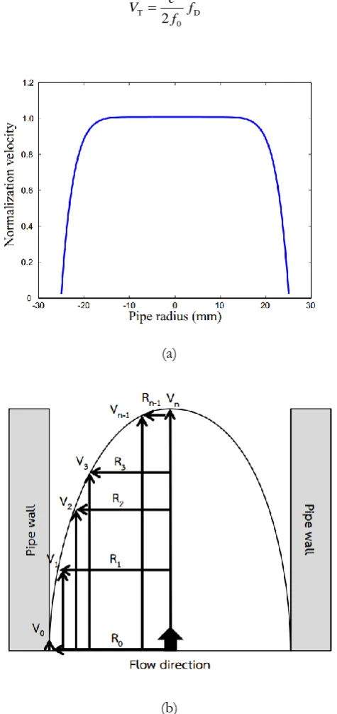
pipe (b) Schematic diagram of accurate flowrate computation from velocity profiles.

(3)

(a)

(b)

Fig. 2. Velocity profiles (a) Normalized velocity profiles of shear thinning fluid flowing in a 50-mm-diameter.

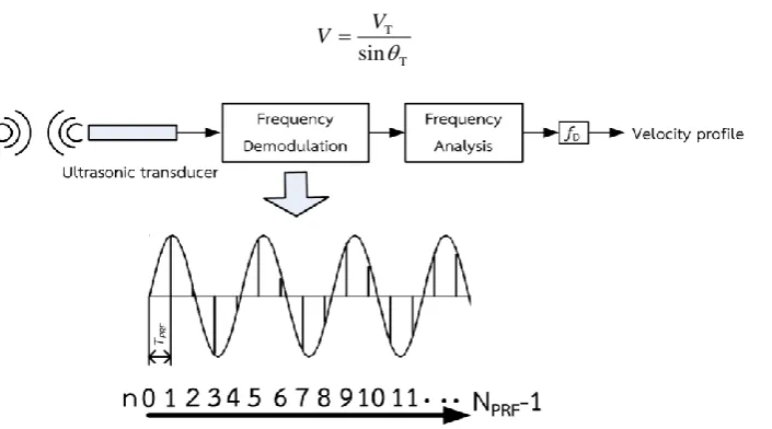
By assuming a directional flow parallel to the streamline, a velocity in flow direction (V) can be determined as Eq. (4):

T D

0

2

c

V f

f

T T

sin

V V



 (4)

Fig. 3. Block diagram of the Doppler-shift measurement system.

In fluids such as water, oil, or incompressible fluid, the viscosity is independent of the shear rate in the radial direction. When fluids flow in a pipe under laminar conditions, a parabolic velocity profile is directly developed as shown in Fig. 1. In particular, if the viscosity decreases for increasing shear rate, this is called a shear thinning behavior. The power law model can describe the shear thinning characteristics [23] as follows:

1/ ( 1) /

( ) 1

1 1/ 2

n n n

R R P r

V r

n K L R



 



   

 _{ } _ _{ } _

    _   _ (5)

V(r) is the velocity profile on any radius (r) as a function of the parameters K and n involving the behavior

of the fluid, the pipe radius R, the pressure drop ΔP, over the axial distance ΔL. A velocity profile

according to shear thinning in a 50-mm-diameter pipe is shown in Fig. 2(a). Flowrate measurement requires only an ultrasonic transducer with the measuring line passing through the center of the pipe. An accurate flow rate (Qv) can be realized precisely by integrating only half of the velocity profile as follows:





3 3 2 3 3

2 0 1 i+1 i+2

V 0 i+1 i n n

0

0 1 i+1 i+2

3

n

i

R R R R

Q V V V R V

R R R R

 



   

 _    _

 





where Ri is the distance from the pipe center to the calculating point, and Vi is the velocity of the point as

shown in Fig. 2(b).

3.

Signal Processing Methods

Figure 3 illustrates a block diagram of the Doppler-shift frequency measurement. The echo signal is modeled by Eq. (7) [8] as:

1

0 0

( ) prf sin 2 [ ]

N

D

n n

n prf

f n

s t A f t t w n

f







 

 _   _

 



where tn represents the delay time of the echo at nth pulse, An is an amplitude, and w[n] is a noise signal.





 ₀  

( ) 2 ( )exp( 2 ) LowPass I( ) Q( )

z t s t i f t x t ix t (8)

where xI(t) and xQ(t) are real and imaginary of z(t). 3.1. The Fast Fourier Transform Method

Since the Doppler-shift frequency of the echo is derived from the velocity, the determination of the peak frequency can be selected using the FFT output magnitude as:

 2  2

( ) ( ) ( )

mag I Q

X f X f iX f (9)

where XI(f) and XQ(f) are the discrete Fourier transforms of xI(t) and xQ(t). FFTs are carried out for each

channel to express the power spectrum of the frequency as Eq. (10).

2 2

2 2

( ) (Re[ ( )] Im[ ( )]) (Re[ ( )] Im[ ( )])

( ) (Re[ ( )] Im[ ( )]) (Re[ ( )] Im[ ( )])

f I Q Q I

b I Q Q I

P f X f X f X f X f

P f X f X f X f X f

   

    (10)

Pf and Pb are power spectra of forward direction and backward direction respectively. The Doppler

frequency can be computed by averaging the spectrum as follows:









f b

k

f P f P f

f

P f P f

    





3.2. The Autocorrelation Method

This method demonstrates a time domain analysis to calculate the phase difference between consecutive received signals. The autocorrelation (Rm) derived from the sampled time domain signal (z[n]) of Eq. (8) is

expressed as follows:









[ ] [ 1]

[ ] [ 1] [ ] [ 1]

[ ] [ 1] [ ] [ 1]

prf

prf

prf

N

m m m

n N

m I I Q Q

n N

I Q I Q

n

m A B

R z n z n

R x n x n x n x n

i x n x n x n x n

R R iR

                  







and the Doppler frequency can then be defined in Eq. (13) as:

   1 , 1 _tan 2 B D AC prf A R f

T R (13)

3.3. The Maximum Likelihood Estimation Method

 

    

[ ] sin(2 D ) [ ] 0,1,2,..., prf 1

z n A f n w n n N (14)

The probability density function (PDF) is

























/2 2

2

0

1

1

( [ ]; , , )

exp[

( [ ]

sin(2

)) ]

2

(2

)

prf

prf

N

D N D

n

p z n A f

z n

A

f n

where σ2 _{is the variance of the noise signal. The MLE in Eq. (15) can be maximized when minimizing the}

term of (z[n] – Asin(2πfDn + ϕ))2 and assuming that F(A,fD,ϕ) = Σ (z[n] – Asin(2πfDn + ϕ))2 then,

















, , ( ( ) (cos sin(2 ) sin cos(2 ))

( ) sin(2 ) cos(2 )

prf

prf

N

D D D

n N

D D

n

F A f z n A f n f n

z n C f n C f n

(16)

C1 is Acosϕ and C2 is Asinϕ. Then, from the square of C1 and C2, the two unknown parameters, A and ϕ,

can be expressed as:

 2 2

1 2

A C C (17)

_ 1 2 1

tan C

C (18)

Next, we assume this definition,

[ ] 1 cos(2 [1]) cos(2 [2]) cos(2 [ 1])

[ ] 1 sin(2 [1]) sin(2 [2]) sin(2 [ 1])

T

D D D prf

T

D D D prf

y n f f f N

x n f f f N













and insert C1, C2, x[n] and y[n] into Eq. (16) to give Eq. (19) as:











1 2 1 2

0 1 2 , , ( [ ] [ ] [ ]) , , ( ( prf N D n T D

F C C f z n C x n C y n

F C C f z HΛ z HΛ

(19) where,













 _{1 2}

[0] [1] [2] [ 1]

[ ] [ ]

T

T

z z z z n

y n x n

C C

z H Λ

ˆΛ can be estimated by minimizing Eq. (19).



 

_{ }  1

1 2

ˆ ˆ ˆ T _{( )}

T T

C C

Λ H H H z (20)





  - 1

1 2

ˆ ˆ_{, ,} T_{( (} T ₎ T₎

D

F C C f z I H H H H z (21)

Table 1. Comparison of the CRLB and variance of estimators for 20.00 dB SNR.

Estimation fD,MLE (kHz)

Actual parameter 1

Mean 1.00023

variance 1.6126 x 10-6

CRLB 7.0258 x 10-7

I is an identity matrix and _{I - H(H H) H}T -1 T_{is an idempotent matrix. To estimate f}

D, we need to maximize

T T -1 T

z (I - H(H H) H )z over a frequency region as:

 

 - 1

,

ˆ _{max( ( ( ) ) )}

D

T T T

D MLE _{f f}

f z I H H H H z (22)

The lowest possible variance of an unbiased frequency estimator can be guaranteed using the Cramer-Rao lower bound (CRLB) [24]. The CRLB is equal to the inverse of the Fisher matrix defined as follows

         2

, 2 2 2 2

2

1 12

ˆ

var( )

ln ( [ ]; , , ) 2 ( 1)

[ ]

D MLE

D prf prf

D f

p z n A f A N N

E

f

(23)

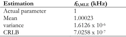
Since the unknown frequency of MLE is embodied in the observed data and the underlying PDF (assumed as noise), the frequency estimator is referred to as the uniformly minimum variance unbiased estimator to emphasize that the variance is smallest for all frequencies. To assess the performance of the estimator, a Monte-Carlo simulation was utilized to investigate a mean and variance against the CRLB. One kHz of the Doppler-shift frequency added to a basic frequency (4 MHz) represented approximately 0.9 m/s of the particle’s velocity. A Monte-Carlo simulation on 100 trials of repeating 100 MHz sampling was performed. Comparison of the CRLB and variance of estimators on 20 dB of signal-to-noise ratio (SNR) is shown in Table 1. In this case, the theory of the CRLB is similar to the variance of the frequency estimator.

3.4. Multiple Signal Classification Method

The observed data set x[n] was extracted from the frequency demodulation including the three unknown parameters and noise as Eq. (24).

[ ] exp( 2 D ) [ ] 0,1,2, , prf 1

v n  i  f n w n n N  (24)

γ is a complex number representing an amplitude and phase, w[n] is a noisy signal, and v[n] is correlated to itself and the covariance matrix is expressed as follows:

*

[ ] ( [ ] [ ])

( [ ] [ ])

v

H

v v v

r m E v n v n m E r m r m

  

 

R (25)

where rv[m] is a correlation function of each m, m is a lack number, E( ) is expectation, and H is a conjugate

transpose. Rv is decomposed into eigenvectors and eigenvalues using the singular value decomposition as

expressed in Eq. (26) as:

H v 

U is an eigenvector matrix and V is an eigenvalue matrix. The covariance matrix in Eq. (25) includes a pure

signal datum and a noise datum. Therefore, V can be rewritten as eigenvalues of both pure signal and noise,

with only eigenvalue (λi) dependent on the signal space as follows:





 _



 

 _ 

 



 

 _ 

 

1

2

0 0 0 0

0 0 0 0

0 0

0 0 M 0 _{M M}

V (27)

Frequency decomposition can contribute using the definition of the noise subspace and the signal vector. To do so, M = L+1 is set when the dimension of the noise subspace Un from UMxM of the covariance

matrix is L, dim(Un) = MxL. The signal eigenvector e(ωk) of the kth frequency component is orthogonal to

the noise subspace as:





 ( ) H( ) 0

n k k n

U e e U (28)

where e(ωk) = [1, exp(iωk), exp(i2ωk), …, exp(i(M-1)ωk)]. Then, artificial spectra can be obtained by

evaluating an annihilating filter at different frequencies as follows:





 1 ₂

ˆ( )

( )

k j

H k n

P e

e U (29)

This is called the pseudo spectra, which have peaks where the zeros are. Finally, the Doppler-shifted frequency can be computed on the peak maximization as:

; max ( k)

j D MUSIC _{f k}

f P 



 e (30)

3.5 Estimation of Signal Parameter via Rotational Invariance Technique Method

Without loss of generality, we again assume a sinusoidal signal corrupted by noise as:

 

    _prf 

[ ] cos(2 D ) [ ] 0,1, 2, , 1

z n A f n w n n N (31)

The autocorrelation and covariance matrix of z[n] is given by Eq. (25), with eigenvalues and eigenvectors decomposed by Eq. (26). Now, two matrices are defined as follows:

1 1 ( 1) 1 ( 1)

2 ( 1) 1 1 ( 1)

[ ]

[ ]

M M M M

M M M M

    

    

 

Γ I 0

Γ 0 I (32)

The first and last (M-1) columns of an (MxM) matrix are used and called the selector matrices.

1 1 2 2

S = Γ U

S = Γ U (33)

The rotational invariance for the matrices in Eq. (33) can be written compactly as:

1 2

where Φ = [1, exp(iω1), exp(iω2), …, exp(iωk)], and is invariant to transformation using some unitary matrix T.

1 2

H

1 2

1 2

Γ (UT)Φ = Γ UT

Γ UTΦT = Γ U

Γ UΨ = Γ U

(35)

where Ψ = TΦTH. The eigenvalues computed in Ψ are definitely equal to those in Φ. To solve the rotational invariance formula, the least-squares solution was used as follows:

H H -1

1 1 1 2

Ψ =(U Γ Γ U) UΓ Γ U (36)

The largest eigenvalue λD represents an estimate of the frequency factors exp(iωD), where













 1 

, prf

arg( )

cos ( ) 2

D D

D D ESPRIT

f f (37)

4.

Experimental Comparison

4.1. Experimental Setup

In general, reflection for UVP is an issue involving the study of sound propagation in water. The ultrasound waves generated by the pulser/receiver can move through the pipe wall, water, and particles as longitudinal waves and also as transverse waves in solids. The ultrasound can travel through any object only if its own wave length is smaller than the object size. Reflection is a change in direction of a wavefront at an interface between two different media to return from an original point that the ultrasound is produced. Nowadays, there have been many researches adopting the ultrasound reflection, for examples, echolocation, NDT, and medicine. Not only UVP was used for the flow profile evaluation on a single phase flow, but it was also applied as a tool of assessing on a bubbly flow [25].

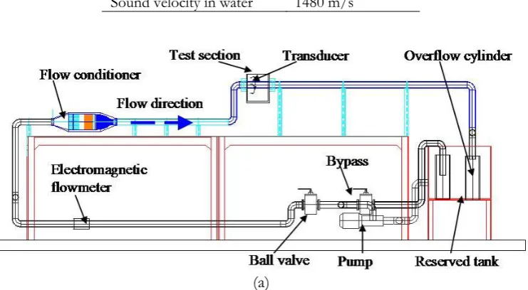
To verify the candidate methods, the effects of Nprf, fprf, and flowrate tested on the experimental station

(38)

where ρ is density, u and v are velocity components, p is pressure, and μ is dynamic viscosity. Computer

simulation (FLUENT 12.0) was verified to visualize the location of the test station and ensure that the stream line had a fully developed flow, at 20 times the dimeter (20D), as shown in Fig. 4(c). The UVP system measured the velocity along the ultrasonic measuring line, so the ultrasonic probe was installed inside the test section at incident angle 45 degrees. The velocity inside the pipe wall could not be estimated due to physical limitations.

Table 2. UVP fluid parameter configuration.

Parameter Configuration

Fluid Water

Fluid temperature 20°C ±2°C

Fluid flow rate

Reynolds number 20 L/min and 3 L/min 9,522 at 20 L/min 1,421 at 3 L/min

Tracking particle Nylon particle 80 µm

Table 3. UVP transducer parameter configuration.

Parameter Configuration

Basic frequency

Number of cycles 4MHz 4

Pulse repetition frequency 4KHz and 8KHz

Number of repetition 32, 64 and 128

Spatial resolution

Sound velocity in water 0.74 mm 1480 m/s

(a)





 

 

 

0

u v

x y

p u u

uu vu

x y x x x y y

p v v

uv vv

x y y x x y y

















 _ _

 

 



 _  _{  }    _{ } 



 

        _  _

 



 _  _{  }    _{ } 



 

(b)

(c)

Fig. 4. Schematic illustration for (a) Experimental apparatus of double pipe flow (b) Ultrasonic velocity profile measurement system (c) Location of the test section including a velocity profile at 20 L/min.

4.2. Experimental Results

The UVP determined by the proposed methods was evaluated repeatedly with 1000 trials, and then averages and standard deviations were compared experimentally in each situation. There was an important constraint on the maximum detectable velocity fprf [4], given by

4 0 max

prf

f v f

c (39)

The high flowrate was set at 20 L/min (Vmax = 0.22 m/s). The smallest frequency of repetitions for

antialiasing was 2.37 kHz. The pulser/receiver used in this experiment was varied at fprf = 2, 4, and 8 kHz.

Accordingly, fprf was conditioned at 4 and 8 kHz because at 2 kHz fprf was aliasing. UVP was recorded by

Figures 5 (a), (b), and (c) show the results of averaged UVP at a constant fprf = 8 kHz and varying Nprf =

32, 64, and 128. In Figs. 5 (a), (b), and (c), averaged UVPs approached the true value at Nprf = 32, 64 and

128 of all methods except only MUSIC which showed greater variance than the others as shown in Table 4, and lowering Nprf of MUSIC reflected to decreasing accuracy. For ESPRIT, the standard deviation was

marginally low at Nprf = 128, and Nprf was corresponding to errors since decreasing Nprf was directly

proportional to lower accuracy. In the case of AC, it seemed that Nprf was not consistent with errors

because decreasing Nprf led to higher accuracy of fprf = 8 kHz. Velocity profiles of FFT and MLE, when

considering Nprf = 64 and 128, were close to the theoretical profile. Generally speaking, averaged UVP of fprf

= 8 kHz exhibited a large difference with decreasing Nprf = 32 and accuracy was confirmed that the higher

Nprf, the lower precision was given. Next, the pulser/receiver was adjusted to observe the effect when fprf

was equal to 4 kHz. At fprf = 4 kHz the averaged UVP was smoother than at fprf = 8 kHz as shown in Figs. 5

(d), (e), and (f). MUSIC still had the greatest error of approximately 9%. For AC, there was no effect of Nprf

since all Nprf of fprf = 4 kHz provided the same errors of approximately 3%. Nprf was not only inconsistent

with accuracy of AC, but it did with FFT and MLE as well. FFT and MLE had errors of approximately 3% and 4%, respectively. For ESPRIT, it still had consistency of decreasing Nprf to lower accuracy as well as a

case of fprf = 8 kHz. To make a measure of how spread out profiles were, standard deviations in each

distance are used for dispersion as follows

(40)

where vi is an individual value, u is the averaged value, and N is the total number of profiles. Standard

deviations of 4 kHz were indicated in Table 4, MUSIC showed the highest deviation of all methods while adjusting fprf = 8 kHz had higher standard deviation than fprf = 4 kHz. For MLE, Nprf and fprf did not

significantly affect standard deviation since standard deviation was stable. AC provided the lowest standard deviation at Nprf = 128 of both frequencies. FFT agreed with MUSIC in that increasing frequency produced

the higher deviation. For ESPRIT, decreasing Nprf affected to higher deviation while the higher frequency

fprf = 8 kHz had greater standard deviation than the lower one fprf = 4 kHz. In term of quality, FFT that

produces the minimum error and variance was considered as the appropriate situation Nprf = 128 and fprf =

8 kHz for high flowrate.

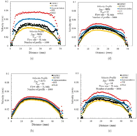
For the next test, verification was carried out by determining the capability of detecting a low flow rate (Qv =3 L/min.) to fully evaluate the effects. Figure 8 and Table 5 compare averaged UVP and standard

deviation for the proposed techniques at different Nprf of low flow rate at a constant fprf = 8 and 4 kHz. In

Figs. 7 (a), (b), and (c), the profiles indicated that MLE had the greatest profile of repetitions because its shape provided the ability to realize velocity profiles at all Nprf . Other methods had the misty velocity

profile. However, velocity profiles of all methods showed better behavior when Nprf was adjusted to the

higher sample Nprf = 128. FFT was the worst case scenario as its velocity profile could not be realized in

Nprf = 32 and fprf = 8 kHz of low flow rate. When the pulser/receiver was set to have decreasing fprf = 4 kHz,

averaged UVP had better satisfaction as shown in Figs. 7 (d), (e), and (f). MLE still gave the best response of velocity profile covering all situations of Nprf = 32, 64, and 128. ESPRIT, AC, and MUSIC recorded

smoother velocity profiles if samples were varied at least to Nprf = 64. Figure 8 shows bar graphs in a form

of percentage error involving a low flow rate. FFT and AC gave large errors between the true and computed values in all situations under a low flow rate, and they could not be accepted as candidates for ultrasonic velocity profiles. For ESPRIT, it appeared that Nprf had no effect on velocity estimation but

accuracy tended to a higher error than 10% of fprf = 8 kHz and 5% of fprf = 4 kHz. MLE showed an error

less than 5 % of reading accuracy, while MUSIC results gave approximately 12% of error at fprf = 4 kHz.

Therefore, MLE was appropriate for use to visualize low velocity profiles. MLE that produces the minimum error and variance was considered as the appropriate situation Nprf = 128 and fprf = 4 kHz for the

given conditions for low flowrate. Table 6 is the summary of the suitable condition in which the algorithm keeps minimum error.

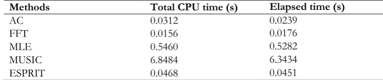
The amount of time for which a central processing unit (CPU) was used for processing instructions of algorithms was assessed. In addition, elapsed time, the amount of time passing from the start of an event to its finish, was used to evaluate computation time. Intel (R) Core (TM) i5-2410 M CPU @ 2.30 GHz and Windows 7 Ultimate 64 bit operating system were used for calculation. Table 7 shows total CPU and elapsed times of each candidate method. The lower the value of total CPU time, the less time they took to





 







1

1 1000

N i i

solve the solution. FFT, AC, and ESPRIT took much less time than MLE and MUSIC. MUSIC was not appropriate for real-time measurement because it required at least 5 seconds for computation.

(a) (d)

(c) (f)

Fig. 5. Averaged UVP at Raynolds number = 9522 and flowrate = 20 liters/minute with varying Nprf and

fprf: (a) Nprf = 32, fprf = 8 kHz (b) Nprf =64, fprf = 8 kHz (c) Nprf = 128, fprf = 8 kHz (d) Nprf = 32, fprf = 4 kHz

(e) Nprf = 64, fprf = 4 kHz (f) Nprf = 128, fprf = 4 kHz.

(a)

(b)

Fig. 6. Error of flowrate measurement at Qv = 20 L/min (a) fprf = 8 kHz (b) fprf = 4 kHz.

0 2 4 6 8 10 12 14

AC FFT MLE MUSIC ESPRIT

Signal processing methods

Flowrate measurement at Q

= 20 L/min and

f

=8 kHz

32 64 128

%

Err

or

N

0 2 4 6 8 10 12

AC FFT MLE MUSIC ESPRIT

%

Err

or

Signal processing methods

Flow measurement at Q

= 20 L/min and

f

= 4 kHz

32 64 128

Table 4. Comparison of standard deviation on velocity profiles at flowrate Qv = 20 L/min with 1000 trials.

Methods Standard deviation (m/s)

Nprf = 32 Nprf = 64 Nprf = 128

8 kHz 4 kHz 8 kHz 4 kHz 8 kHz 4 kHz

AC 0.020 0.018 0.019 0.019 0.016 0.015

FFT 0.026 0.018 0.022 0.018 0.016 0.015

MLE 0.021 0.020 0.020 0.020 0.020 0.021

MUSIC 0.044 0.038 0.043 0.029 0.032 0.026

ESPRIT 0.028 0.018 0.028 0.018 0.015 0.015

(a) (d)

(c) (f)

Fig. 7. Averaged UVP at Raynolds number = 1421 and flowrate = 3 liters/minute with varying Nprf and fprf:

(a) Nprf = 32, fprf = 8 kHz (b) Nprf =64, fprf = 4 kHz (c) Nprf = 64, fprf = 8 kHz (d) Nprf = 64, fprf = 4 kHz (e)

Nprf = 64, fprf = 4 kHz (f) Nprf = 128, fprf = 4 kHz.

(a)

(b)

Fig. 8. Error of flowrate measurement at Qv = 3 L/min (a) fprf = 8 kHz (b) fprf = 4 kHz.

0 20 40 60 80 100 120 140

AC FFT MLE MUSIC ESPRIT

Signal processing methods

Flowrate measurement at Q

= 3 L/min and

f

= 8 kHz

32 64 128

%

Err

or

N

0 10 20 30 40

AC FFT MLE MUSIC ESPRIT

%

Err

or

Signal processing methods

Flow measurement at Q

= 3 L/min and

f

= 4 kHz

32 64 128

Table 5. Comparison of standard deviation on velocity profiles at flowrate Qv = 3 L/min with 1000 trials.

Methods Standard deviation (m/s)

Nprf = 32 Nprf = 64 Nprf = 128

8 kHz 4 kHz 8 kHz 4 kHz 8 kHz 4 kHz

AC 0.015 0.010 0.010 0.008 0.008 0.006

FFT 0.035 0.012 0.018 0.008 0.010 0.006

MLE 0.012 0.008 0.010 0.006 0.008 0.006

MUSIC 0.020 0.010 0.012 0.010 0.010 0.008

ESPRIT 0.040 0.020 0.031 0.016 0.022 0.010

Table 6. Suitable condition in each method.

Methods High flow (20 L/min.) Low flow (3 L/min.)

fprf Nprf fprf Nprf

AC 8 kHz 32 4 kHz 128

FFT 8 kHz 128 4 kHz 128

MLE 8 kHz 128 4 kHz 32

MUSIC 8 kHz 128 8 kHz 32

ESPRIT 8 kHz 128 4 kHz 64

Table 7. Total CPU and elapsed times for computation of one profile.

Methods Total CPU time (s) Elapsed time (s)

AC 0.0312 0.0239

FFT 0.0156 0.0176

MLE 0.5460 0.5282

MUSIC 6.8484 6.3434

ESPRIT 0.0468 0.0451

4.3. Discussions

Accuracy of velocity profiles could be classified as high flows and low flows. All methods except MUSIC had errors not over than 4% in the case of high flows. Nprf was not a main factor of lowering accuracy

because almost all methods had smaller error in order of increasing Nprf from least to most but except AC.

If considering on fprf, it appeared that AC, FFT, and MLE had higher accuracy but MUSIC and ESPRIT

did not. For low flows, MLE and MUSIC had the smallest error of fprf = 8 kHz, and the error was lower

than 5%. They were appropriate to be used for the signal processing tool for low flows. If considering the optimal methods of both high and low flow rates, MLE provided smaller error and variance. The main reason why the MLE gave appropriate results over than the others assumed that a signal space was composed of two identical subarrays, and an array element was a member of both subarrays. This leaded to the rotational invariance of signal subspace spanned by the data vector associated with the spatially displaced subarrays to find a frequency. However, ESPRIT estimates frequency by means of the least-squares solution referred in Eq. (36), not scanning. The least-least-squares solution may lead to a vital reason of divergence, and why ESPRIT results had difficulty of estimating frequency, similar to AC at a low flow. MUSIC used a hybrid method of eigenvalue decomposition to classify only signal vectors from noise vectors and scanning frequency. The noise vectors were then used for searching frequency spectra. Therefore, while low Nprf were given, the signal vector identified using eigenvalue decomposition was not

5.

Conclusions

Comparative ultrasonic velocity profiles were studied by implementing AC, FFT, MLE, MUSIC, and ESPRIT. Experiments were carried out to investigate the effects of flow rate, number of repetitions, and frequencies of repetitions for use in the fluid mechanics field. Velocities were analyzed under varying fprf and

Nprf of a pulser/receiver. Both appropriate fprf and Nprf must be chosen depending on the flow rate

condition. More accurate results could be obtained by increasing the number of pulse repetitions to at least

Nprf= 64, and the best at Nprf = 128 and fprf = 8 kHz for high flow. For low flow, the suitable fprf was 4 kHz

but Nprf could not be decided. MUSIC responsed to both only low flow rates but at high flow the error was

unacceptable. AC and FFT were appropriate for only the high flowrate condition. ESPRIT had suitable in high flow but at low it was appearance that there was only fprf = 4 kHz of all Nprf to keep low errors. MLE

was relatively unaffected by the flow condition. FFT, AC, and ESPRIT took much less computational time than MLE and MUSIC. Although AC and FFT had the remarkable ability of both accuracy and low time computation, it was useful only at high flow. Accordingly, MLE was selected as the algorithm of choice for measuring UVP in terms of efficiency.

Acknowledgments

This work was undertaken following a memorandum of understanding involving research operations between King Mongkut’ University of Technology North Bangkok, Tokyo Institute of Technology, and Office of Atoms for peace, Ministry of Science and Technology.

References

[1] Endress and Hauser, “Flow measuring principles,” in Flow Handbook, 3rd ed. Switzerland: Schaub Medien; Endress Hauser, 2006, ch. 3, pp. 49–171.

[2] Y. Inoue, H. Kikura, H. Murakawa, M. Aritomi and M. Mori, “A study of ultrasonic propagation for ultrasonic flow rate measurement,”Flow. Meas. Instrum., vol. 19, pp. 223-232, Aug., 2008.

[3] Y. Takeda, “Development of an ultrasound velocity profile monitor,” Nucl. Eng. Des., vol. 126, pp.

227-284, Apr. 1991.

[4] T. Ihara, H. Kikura, and Y. Takeda, “Ultrasonic velocity profiler for very low velocity field,” Flow.

Meas. Instrum., vol. 34, pp. 127-133, Dec. 2013.

[5] K. Tezuka, M. Mori, T. Suzuki, and T. Kanamine, “Ultrasonic pulse-Doppler flow meter application for hydraulic power plants,”Flow. Meas. Instrum., vol. 19, pp. 155-162, Aug. 2008.

[6] F. Adba, A. Azbaid, D. Ensminger, S. Fisher, P. François, P. Schmitt, and A. Pallarès, “Ultrasonic device for real-time sewage velocity and suspended particles concentration measurements,” Water. Sci. Technol., vol. 60, pp. 117-125, 2009.

[7] W. Treenuson, N. Tsuzuki, H. Kikura, M. Aritomi, S. Wada, and K. Tezuka, “Accurate flowrate measurement on the double bent pipe using ultrasonic velocity profile method,” Journal of the Japanese

Society for Experimental Mechanics, vol. 3, no. 2, pp. 200-211, Jun. 2013.

[8] H. Murakawa, K. Sugimoto, and N. Takenaka, “Effect of the number of pulse repetitions and noise on the velocity data from the ultrasonic pulsed Doppler method with different algorithms,” Flow. Meas.

Instrum., vol. 40, pp. 9-8, Dec. 2014.

[9] R. G. Lyons, “Digital signal processing tricks,” in Understanding Digital Signal Processing, 2nd _ed.

Massachusetts, 2004, ch. 13, pp. 471–578.

[10] C Kasai, K Namekawa, A. Koyano, and R. Omoto, “Real-time dimensional blood flow imaging using an autocorrelation technique,” IEEE Trans. Sonics Ultrasonics, vol. SU-32, pp. 458 – 464, 1985.

[11] Y. Takeda, “Velocity profile measurement by ultrasonic Doppler method,” Experimental Thermal and

Fluid Science, vol. 10, pp. 444-453, 1995.

[12] I. Guler and E. D. Ubeyli, “Implementing wavelet/probabilistic neural networks for Doppler ultrasound blood flow signals,” Expert. Syst. Appl., vol. 33, pp. 162-170, 2007.

[14] N. Thong-un, W. Wongsaroj, W. Treenuson, J. Chanwutitum, and H. Kikura, “Doppler frequency estimation using maximum likelihood function for low ultrasonic velocity profile,” Acoust Sci Technol., vol. 38, no. 5, pp. 268 - 271, Sep. 2017.

[15] R. O. Schmidt, “Multiple emitter location and signal parameter estimation,” IEEE Trans. Antennas

Propag., vol. AP-34, pp. 276-280, 1986.

[16] K. Muzutani, T. Ito, M. Sugimoto, and H. Hashisume, “TSaT-MUSIC: A novel algorithm for rapid

and accurate ultrasonic 3D localization,” EURASIP J Adv. Signal. Process., vol. 101, Dec. 2011.

[17] Y. Zhong, S. Yuan, and L. Qiu, “Multiple damage detection on aircraft composite structures using near-field MUSIC algorithm,” Sens. Actuators. A Phys., vol. 214, pp. 234-244, Aug. 2014.

[18] A. Paulraj, R. Roy, and T. Kailath, “Estimation of signal parameter invariance technique—ESPRIT,”

19th _{Asilomar Conference on Circuits, System and Computers, 1985, pp. 83-89.}

[19] R. Roy and T. Kailath, “ESPRIT-estimation of signal parameters via rotational invariance techniques,”

IEEE Trans. Acoust. Speech Signal Process., vol. 37, pp. 984-995, Jul. 1989.

[20] Z. Chen, G. Gokeda, and Y. Yu, “DOA estimation with ESPRIT algorithm,” Introduction to

Direction-of-Arrival Estimation, 1st _{ed. Boston, 2010, ch. 5, pp. 81–122.}

[21] G. Guidi, L. Corti, and H. Tortobi “Application of autoregressive methods to multigate spectral analysis,” Ultrasound Med., vol. 26, no. 4, pp.585-592, May 2000.

[22] S. Ricci, “Adaptive spectral estimators for fast flow-profile detection,” IEEE Trans. Ultrason., Ferroelect.,

Freq. Control., vol. 60, no. 2, pp.421-427, Feb. 2013.

[23] S. Ricci, M. Liard, B. Birkhofer, D. Lootens, A. Bruhwiler, and P. Tortoli, “Embedded Doppler system for industrial in-line rheometry,” IEEE Trans. Ultrason., Ferroelect., Freq. Control., vol. 59, no. 7, pp.1395-1401, Jul. 2012.

[24] N. Thong-un, S. Hirata, Y. Orino, and M. K. Kurosawa, “A linearization-based method of simultaneous position and velocity measurement using ultrasonic waves,” Sens. Actuators. A Phys., vol. 233, pp. 480-299, Aug. 2015.

[25] W. Wongsaroj, A. Hamdani, N. Thong-un, H. Takahashi, and H. Kikura, “Ultrasonic measurement of velocity profile on bubbly flow using fast Fourier transform (FFT) technique,” IOP Conf. Ser.: Mater.

Sci. Eng., vol. 249, no. 1, p. 012011, 2017.

[26] Y. Takeda, N. Furuichi, M. Mori, M. Aritomi, and H. Kikura, “Development of a new flow metering system using UVP (Preliminary performance assessment using NIST flows standards),” in ASME

Fluids Engineering Division Summer Meeting, 2000.