A Binary Neural Decision Table Classifier

This is a repository copy of A Binary Neural Decision Table Classifier.

White Rose Research Online URL for this paper:

http://eprints.whiterose.ac.uk/89520/

Version: Submitted Version

Conference or Workshop Item:

Hodge, Victoria Jane orcid.org/0000-0002-2469-0224, O'Keefe, Simon

orcid.org/0000-0001-5957-2474 and Austin, Jim orcid.org/0000-0001-5762-8614 (2004) A

Binary Neural Decision Table Classifier. In: Proceedings Brain Inspired Cognitive Systems

2004 (BICS 2004), 29 Aug - 01 Sep 2004.

[email protected] https://eprints.whiterose.ac.uk/

Reuse

Items deposited in White Rose Research Online are protected by copyright, with all rights reserved unless indicated otherwise. They may be downloaded and/or printed for private study, or other acts as permitted by national copyright laws. The publisher or other rights holders may allow further reproduction and re-use of the full text version. This is indicated by the licence information on the White Rose Research Online record for the item.

Takedown

If you consider content in White Rose Research Online to be in breach of UK law, please notify us by

A Binary Neural Decision Table Classifier

Victoria J. Hodge

Simon O’Keefe

Jim Austin

[email protected]

[email protected]

[email protected]

Advanced Computer Architecture Group

Department of Computer Science

University of York, York, YO10 5DD, UK

Abstract

In this paper, we introduce a neural network-based

decision table algorithm. We focus on the

implementation details of the decision table algorithm when it is constructed using the neural network. Decision tables are simple supervised classifiers which, Kohavi demonstrated, can outperform state-of-the-art classifiers such as C4.5. We couple this power with the efficiency and flexibility of a binary associative-memory neural network. We demonstrate how the binary associative-memory neural network can form the decision table index to map between attribute values and data records. We also show how two attribute selection algorithms, which may be used to pre-select the attributes for the decision table, can easily be implemented within the binary associative-memory neural framework. The first attribute selector uses mutual information between attributes and classes to select the attributes that classify best. The second attribute selector uses a probabilistic approach to evaluate randomly selected attribute subsets.

Introduction

Supervised classifier algorithms aim to predict the class of an unseen data item. They induce a hypothesis using the training data to map inputs onto classified outputs (decisions). This hypothesis should then correctly classify previously unseen data items. There is a wide variety of classifiers including: decision trees, neural networks, Bayesian classifiers, Support Vector Machines and k-nearest neighbour (k-NN).

We have previously developed a k-NN classifier[HA04] using an associative memory neural network called the Advanced Uncertain Reasoning Architecture (AURA)[A95]. In this paper, we extend the approach to encompass a decision table supervised classifier, coupling the classification power of the decision table with the speed and storage efficiency of an associative memory neural network

The decision table has two components: a schema and a body. The schema is the set of attributes pre-selected to represent the data and is usually a subset of the data’s

total attributes. There are various approaches for attribute selection; we discuss two later in this paper. The body is essentially a table of labelled data items where the attributes specified by the schema form the rows and the decisions (classifications) form the columns. Each column is mutually exclusive and represents an equivalence set of records as defined by the attributes of the schema. Kohavi [K95] uses a Decision Table Majority (DTM) for classification whereby if an unseen item exactly matches a stored item in the body then the decision table assigns the stored item’s decision to the unseen item. However, if there is no exact match then the decision table assigns the majority class across all items to the unseen item. Our decision table approach implements both DTM and proximity-based matching as implemented in our k-NN classifier whereby if there is no exact match then the decision table assigns the class of the nearest stored item to the unseen item.

RAM-based Neural Networks

The AURA C++ library provides a range of classes and methods for rapid partial matching of large data sets [A95]. In this paper we define partial matching as the retrieval of those stored records that match some or all of the input record. In our AURA decision table, we use best partial matching to retrieve the records that are the top matches.

AURA belongs to a class of neural networks called Random Access Memory (RAM-based) networks. RAM-based networks were first developed by Bledsoe & Browning [BB59] and Aleksander & Albrow [AA68] for pattern recognition and led to the WISARD pattern recognition machine [ATB84]. See also [A98] for a detailed compilation of RAM methods.

RAMs are founded on the twin principles of matrices (usually called Correlation Matrix Memories (CMMs)) and n-tupling. Each matrix accepts m inputs as a vector or tuple addressing m rows and n outputs as a vector addressing n columns of the matrix. During the training phase, the matrix weights Mlkare incremented if both the input row Ij

l

and output column Oj k

Therefore, training is a single epoch process with one training step for each input-output association preserving the high speed. During recall, the presentation of vector

Ij elicits the recall of vector Oj as vector Ij contains all of

the addressing information necessary to access and retrieve vector Oj. This training and recall makes RAMs

computationally simple and transparent with well-understood properties. RAMs are also able to partially match records during retrieval. Therefore, they can rapidly match records that are close to the input but do not match exactly.

AURA

AURA has been used in an information retrieval system[H01], high speed rule matching systems[AKL95], 3-D structure matching[TA00] and trademark searching[AA98]. AURA techniques have demonstrated superior performance with respect to speed compared to conventional data indexing approaches [HA01] such as hashing and inverted file lists which may be used for a decision table body. AURA trains 20 times faster than an inverted file list and 16 times faster than a hashing algorithm. It is up to 24 times faster than the inverted file list for recall and up to 14 times faster than the hashing algorithm. AURA techniques have demonstrated superior speed and accuracy compared to conventional neural classifiers [ZAK99].

The rapid training, computational simplicity, network transparency and partial match capability of RAM networks coupled with our robust quantisation and encoding method to map numeric attributes from the data set onto binary vectors for training and recall make AURA ideal to use as the basis of an efficient implementation. A more formal definition of AURA, its components and methods now follows.

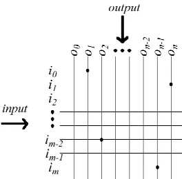
Correlation Matrix Memories (CMMs) are the building blocks for AURA systems. AURA uses binary input I

and output O vectors to train records in to the CMM and recall sets of matching records from the CMM as in Equation 1 and Figure 1.

Equation 1

OR logical is where

all

∨

∨

= _j I_j OT_j CMM

Training is a single epoch process with one training step for each input-output association (each Ij x OTj in

Equation 1) which equates to one step for each record in the data set.

Figure 1 Showing a CMM with input vector i and output vector o. Four matrix locations are set following training i0o0, i2on-2, im-1o0 and imon.

For the methodology described in this paper, we:

• Train the data set into the CMM (decision table body CMM) which indexes all records in the data set and allows them to be matched.

• Select the attributes for the schema using schema CMMs. We describe two selection algorithms. One uses a single CMM and the second algorithm uses two coupled CMMs.

• Match and classify unseen items using the trained decision table.

Data

For the data sets:

• Symbolic and numerical unordered attributes are enumerated and each separate token maps onto an integer (Text Integer) which identifies the bit to set within the vector. For example, a SEX_TYPE attribute would map as, (F 0) and (M 1).

Kohavi’s DTM methodology is principally aimed at symbolic attributes but the AURA decision table can handle continuous numeric attributes.

• Any real-valued or ordered numeric attributes, are quantised (mapped to discrete bins) and each individual bin maps onto an integer which identifies the bit to set in the input vector.

A range of input values for attribute f map onto each bin which in turn maps to a unique integer to index the vector as in Equation 2. The range of attribute values mapping to each bin is equal.

Equation 2

f fk

fk

fi → bins Integer +offset

ℜ _where

(

)

)

(i∈FV_f ∧ Integer_f ≡ bins_f

In Equation 2, offsetf is a cumulative integer offset

offsetf+1 = offsetf +nBinsf, where nBinsf is the number of

bins for attribute f, card is the cardinality,

FVf is the set of attribute values for attribute f,

is a many-to-one mapping and is a one-to-one mapping.

This quantisation (binning) approach aims to subdivide the attributes uniformly across the range of each attribute. The range of values is divided into b bins such that each bin is of equal width. The equal widths of the bins prevent distortion of the inter-bin distances.

Once the bins and integer mappings have been determined, we map the records onto binary vectors. Each attribute maps onto a consecutive section of bits in the binary vector.

For each record in the data set For each attribute

Calculate bin for attribute value; Set bit in vector as in Equation 2;

Each binary vector represents a record from the data set

Body Training

The decision table body is an index of all contingencies and the decision to take for each. Input vectors represent quantised records and form an input Ij to the CMM

during training. The CMM associates the input with a unique output vector OT

j during training that represents

an equivalence set of records. This produces a CMM where the rows represent the attributes and their respective values and the columns represent equivalence sets of records (where equivalence is determined by the attributes designated by the schema). We use an array of linked lists to store the equivalence sets of records and a second array to store the counts of each class for the equivalence set as a histogram. The algorithm is:

1) Input vector to CMM; 2) Threshold at value nF; 3) If exact match

4) Add the record to column list; 5) Add class to histogram;

6) Else train record as next column;

nF is the number of attributes. Steps 1 and 2 are equivalent to testing for an exact match during body recall as described next. Figure 3 shows a trained CMM where each row is an attribute value and each column represents an equivalence set.

Body Recall

The decision table classifies by finding the set of matching records. To recall the matches for a query record, we firstly produce an input vector by quantising the target values for each attribute to identify the bins and thus CMM rows to activate as in Equation 2. To retrieve

the matching records for a particular record, AURA effectively calculates the dot product of the input vector Ik and the CMM, computing a positive

integer-valued output vector Ok (the summed output vector) as

in Equation 3 and Figure 2 & Figure 3.

Equation 3

O

=

I

•

CMM

The AURA technique thresholds the summed output

T k

O to produce a binary output vector as in Figure 2 for

exact match and Figure 3 for a partial match.

Figure 2 Diagram showing the CMM recall for an exact match. The left hand column is the input vector. The dot is the value for each attribute (a value for an unordered attribute or a bin for an ordered numeric attribute). AURA multiplies the input vector by the values in the matrix columns, using the dot product, sums each column to produce the summed output vector and then thresholds this vector at a value equivalent to the number of attributes in the input (6 here) to produce the thresholded attribute vector which indicates the matching column (the middle column here).

classify the unseen record according to the majority class across the data set.

Figure 3 Diagram showing the CMM recall for a partial match. The left hand column is the input vector. The dot is the value for each attribute (a value for an unordered attribute or a bin for an ordered numeric attribute). AURA multiplies the input vector by the values in the matrix columns, using the dot product, sums each column to produce the summed output vector and then thresholds this vector at a value equivalent to the highest value in the vector (5 here) to produce the thresholded attribute vector which indicates the matching column (the middle column here).

For partial matching, we use the Max threshold. L-Max thresholding essentially retrieves at least L top matches. It sets a bit in the thresholded output vector for every location in the summed output vector that has a value higher than a threshold value. The AURA C++ library automatically sets the threshold value to the highest integer value that will retrieve at least L matches. For the AURA decision table, L is set to the value of 1. There will be a bit set in the thresholded output vector indicating the best matching equivalence set. It is then simply a case of looking up the class histogram for this equivalence set in the stored array and classifying the unseen record as the majority class. We note there may be more than one best matching equivalence set so the majority class across all best matching sets will need to be calculated.

Schema Training

In the decision table body CMM, the rows represented attribute values and the columns represented equivalence sets. In the schema CMM used for the first attribute selection algorithm, the rows represent attribute values and the columns represent individual records. For our second attribute selection algorithm, we use two CMMs where the first CMM indexes the second CMM. In the first CMM1, the rows represent

records and the columns represent attribute values. In the second CMM2, the rows represent attribute values

and the columns represent the records. This second CMM2 is therefore identical to the CMM used for the

first attribute selection algorithm

During training for the first attribute selection algorithm and CMM2 of thesecond attribute selection

algorithm, the input vectors Ij represent the attribute

values in the data records. The CMM associates the input with a unique output vector OTj. Each output

vector is orthogonal with a single bit set corresponding to the record’s position in the data set, the first record has the first bit set in the output vector, the second and so on. During training for CMM1, the records

represent the input vectors Ij with a single bit set and

the output vectors OTj represent the attribute values in

the data records. The CMM training process is given in Equation 1.

Schema Attribute Selection

As with Kohavi, we assume that all records are to be used in the body and during attribute selection.

There are two fundamental approaches to attribute selection which are used in classification: a filter approach that selects the optimal set of attributes independently of the classifier algorithm and the wrapper approach that selects attributes to optimise classification using the algorithm. We examine two filter approaches which are more flexible than wrapper approaches as they are not directly coupled to the classification algorithm.

For a data set with N attributes there are O(NM) possible combinations of M attributes which is intractable to search exhaustively. In the following: we use one filter approach (mutual information attribute selection) that examines attributes on an individual basis and another probabilistic filter approach (probabilistic Las Vegas algorithm) that examines randomly selected subsets of attributes.

Mutual Information Attribute Selection

mutual information between class C and each attribute Fj.

The mutual information between two attributes is “the reduction in uncertainty concerning the possible values of one attribute that is obtained when the value of the other attribute is determined”.

For unordered attributes, nFV is the number of distinct attribute values (fi) for attribute Fj and nClasses the

number of classes (C):

Equation 4 = = = • = = ∧ = • = ∧ = = nClasses c i i nFV

i p p

p p I 1 j j i j 1 j ) f F ( ) c C ( ) f F c C ( log ) f F c C ( ) F C, (

For ordered numeric attributes, the technique computes the mutual information between a discrete random variable (class) and a continuous random variable (attribute). It estimates the probability function of the attributes using density estimation. We assume attribute Fj has density f(x) and the joint density of C and Fj is

f(x,y).

Then the mutual information is:

Equation 5 dx p x f x f x f I nClasses c x = = • = • = = 1 j ) c C ( ) ( ) c C , ( log ) c C , ( ) F C, (

Equation 5 requires an estimate of the density function f(x) and the joint density function f(x, C=c). To approximate f(x) and f(x, C=c), we utilise the binning to represent the density which is analogous to the Trapezium Rule for using the areas of slices (trapezia) to represent the area under the graph for integration. We use the bins to represent strips of the probability density function and count the number of records mapping into each bin to estimate the density.

In AURA, for unordered data, the mutual information is given by Equation 6:

Equation 6 • ∧ • • ∧ • = = = n nRowf n nClass nRowf BVc BVf n n nRowf nRowf BVc BVf n n nRowf I i c i i i i i i nClasses c nRowsFV i ) ( log ) ( ) F C, ( 1 1 j

Where nRowsFV is the number of rows in the CMM for attribute Fj, n is the number of records in the data set,

nRowfi is the number of bits set in row fi of the CMM

(the number of records with attribute value fi), BVfi is a

binary vector (CMM row) for fi, BVc is a binary vector

with one bit set for each record in class c, n(BVfi∧BVc)

is a count of the set bits when BVc is logically anded with BVfi and nClassc is the number of records in class

c.

In AURA, for real/discrete ordered numeric attributes, the mutual information is given by Equation 7:

Equation 7 • ∧ • • ∧ • = = = n nRowb n nClass nRowb BVc BVb n n nRowb nRowb BVc BVb n n nRowb I i c i i i i i i nClasses c nB i ) ( log ) ( ) F C, ( 1 1 j

Where nB is the number of bins in the CMM for attribute Fj, n is the number of records in the data set,

nRowbi is the number of bits set in row bi of the CMM

(the number of records that map to bin bi), BVbi is a

binary vector (CMM row) for fi, BVc is a binary vector

with one bit set for each record in class c,

n(BVfi∧BVc) is a count of the set bits when BVc is

logically ANDed with BVbi and nClassc is the number

of records in class c.

The technique assumes independence of attributes and ignores missing values. It is also the user’s prerogative to determine the number of attributes to select.

Probabilistic Las Vegas Algorithm

Liu & Setiono [LS96] introduced a probabilistic Las Vegas algorithm which uses random search and inconsistency to evaluate attribute subsets. For each equivalence set of records (where the records match according to the attributes designated in the schema), consistency is defined as the number of matching records minus the largest number of matching records in any one class. The inconsistency scores are summed across all equivalence sets to produce an inconsistency score for the particular attribute selection.

attributes until some termination condition is met whereby removing an attribute from the subset decreases the discriminatory power of the subset above a pre-specified threshold. A poor attribute choice at the beginning of a forward or backward search will adversely effect the final selection whereas a random search will not rely on any initial choices.

Liu and Setiono defined their algorithm as:

1) nF_best = N;

2) For j = 1 to MAX_TRIES

3) S = randomAttributeSet(seed); 4) nF = numberOfAttributes(S);

5) If(nF < nF_best)

6) If(InconCheck(S,D) < γ)

7) S_best = S; nF_best = nF;

8) End for

Where D is the dataset, N the number of attributes and γ

the permissible inconsistency score. Liu & Setiono recommend setting MAX_TRIES to 77xN5.

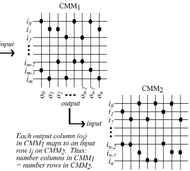
Figure 4 Showing the two CMM combination we use for Liu & Setiono’s algorithm. In the first CMM (CMM1), the records index the rows (one row per record) and the attribute values index the columns_. The outputs from the CMM (matching attribute values) feed straight into the second CMM(CMM2), where the attribute values index the rows _{and the} records index the columns _{(one column per record).}

Liu and Setiono’s algorithm may be calculated simply using the AURA schema CMMs. We need to use two linked CMMs for the calculation as in Figure 4. We rotate the schema CMM (CMM1)through 90º.CMM1’s

rows index the records and CMM1’s columns index the

attribute values. If we feed the outputs from CMM1 (the

activated attribute values) into CMM2 then we can

calculate the inconsistency scores easily. Line 6 of Liu and Setiono’s algorithm listed above then becomes:

Place all records in a queue Q; While !empty(Q)

Remove R the head record from Q; Activate row R in CMM1;

Threshold CMM1 at value 1; Feed CMM1 output into CMM2; Threshold CMM2 at value nF_best;; B = bits set in thresholded_vector; Max = cardinality of largest class; InconCheck(S,D) += B-Max;

End while

The queue effectively holds the unprocessed records. By activating the head record’s row in CMM1 and

Willshaw thresholding at value 1 (denoting all active columns (i.e., all attribute values in the record)), we can determine that record’s attribute values. When these values are fed into CMM2, we effectively activate

all records matching these values. This approach is the most efficient as the CMMs store all attributes and their values but we only focus on those attributes under investigation during each iteration of the algorithm. An alternative approach would be to just store those attributes selected in the random subset each time we execute line 6 of Liu and Setiono’s algorithm but the CMMs would need to be retrained many times (up to 77xN5).

After thresholding CMM2 at the value nFbest (the

number of attributes), we retrieve the equivalence set of matching records where equivalence is specified by the current attribute selection in the algorithm {S}. It is then simply a matter of counting the number of matching records (the number of bits set in the thresholded output vector), calculating the number of these matching records in each class, identifying the largest class membership and subtracting the largest class membership from the number of records.

The algorithm has now processed all of the records in this equivalence set so it removes these records from the queue. If we repeat this process for each record at the head of the queue until the queue is empty, we will have processed all equivalence sets. We can then calculate InconCheck(S,D) for this attribute selection and compare it with the threshold value as in line 6 of Liu and Setiono’s algorithm.

Conclusion

In this paper we have introduced a binary neural decision table classifier. The AURA neural architecture, which underpins the classifier, has demonstrated superior training and recall speed compared to conventional indexing approaches such as hashing or inverted file lists which may be used for a decision table. AURA trains 20 times faster than an inverted file list and 16 times faster than a hashing algorithm. It is up to 24 times faster than the inverted file list for recall and up to 14 times faster than the hashing algorithm. In this paper, we described the implementation details of the technique. Our next step is to evaluate the AURA decision table for speed and memory usage against a conventional decision table implementation.

We have shown how two quite different attribute selection approaches may be implemented within the AURA decision table framework. We described a mutual information attribute selector that examines attributes on an individual basis and scores them according to their class discrimination ability. We also demonstrated a probabilistic Las Vegas algorithm which uses random search and inconsistency to evaluate attribute subsets.

We feel the technique is flexible and easily extended to other attribute selection algorithms.

Acknowledgement

This work was supported by EPSRC Grant number GR/R55101/01.

References

[AA68]

Aleksander, I., & Albrow, R.C. Pattern

recognition with Adaptive Logic Elements. IEE Conference on Pattern Recognition, pp 68-74, 1968.

[ATB84]

Aleksander, I., Thomas, W.V., & Bowden, P.A.

Wisard: A radical step forward in image recognition. Sensor Review, pp 120-124, 1984.

[AA98]

Alwis, S., & Austin, J. A Novel Architecture for Trademark Image Retrieval Systems. In, Electronic Workshops in Computing, 1998.

[A95]

Austin, J. Distributed Associative Memories for High Speed Symbolic Reasoning. In, IJCAI Working Notes of Workshop on Connectionist-Symbolic Integration: From Unified to Hybrid Approaches, pp 87-93, 1995.

[A98]

Austin, J. RAM-based Neural Networks, Progress in Neural Processing 9, Singapore: World Scientific Pub. Co., 1998.

[AKL95]

Austin, J., Kennedy, J., & Lees, K. A Neural Architecture for Fast Rule Matching. In, Artificial Neural Networks and Expert Systems

Conference (ANNES’95), Dunedin, New

Zealand, 1995.

[BB59]

Bledsoe, W.W., & Browning, I. Pattern recognition and Reading by Machine. In, Proceedings of Eastern Joint Computer Conference, pp 225-231, 1959.

[H01]

Hodge, V., Integrating Information Retrieval & Neural Networks, PhD Thesis,Department of Computer Science, The University of York, 2001.

[HA01]

Hodge, V. & Austin, J. An Evaluation of Standard Retrieval Algorithms and a Binary Neural Approach. Neural Networks 14(3), pp. 287-303, Elsevier, 2001.

[HA04]

Hodge, V. & Austin, J. A High Performance k-NN Approach Using Binary Neural Networks. Neural Networks 17(3), pp. 441-458, Elsevier, 2004.

[K95]

Kohavi, R.. The Power of Decision Tables. In, Procs of Eurpean Confernce on Machine Learning. LNAI 914, Springer-Verlag, pp174-189, 1995.

[LS96]

Liu, H., and Setiono, R. A probabilistic approach to feature selection - A filter solution. In, 13th International Conference on Machine Learning (ICML'96), pp. 319-327, 1996.

[TA00]

Turner, A., & Austin, J. Performance Evaluation of a fast Chemical Structure Matching Method using Distributed Neural Relaxation. In, 4th International conference on Knowledge Based Intelligent Engineering Systems, 2000.

[W94]

Wettscherek, D.. A Study of Distance-Based Machine Learning Algorithms. PhD Thesis, Dept of Comp. Sci., Oregon State University, 1994.

[ZAK99]