Explicit Energy-Minimal Short-Term Path Planning
for Collision Avoidance in Crowd Simulation
Saran Sillapaphiromsukaand Pizzanu Kanongchaiyosb,∗
Department of Computer Engineering, Faculty of Engineering, Chulalongkorn University, Bangkok, Thailand
E-mail: a[email protected],b[email protected] (Corresponding author)
Abstract. In traditional crowd simulation methods, global path planning (GPP) and local collision avoidance (LCA) were mostly used to advance pedestrians toward their own goals without colliding. However, we found that using those methods in bidirectional flows can force a pedestrian to get stuck among the incoming people, walk through the congestion, or even unintentionally occupy in a dense area, although more comfortable passageway exists. These odd behaviors are usually produced and simply noticeable in bidirectional case. This paper aims at reducing these artifacts to achieve more behavioral fidelity, by adding the explicit metabolic-energy-minimal short-term path planning (MEM) in between GPP and LCA. For energy analysis, the optimal control theory with the objective energy function from the study of biomechanics was employed, which finally leads to the useful optimal walk-ing characteristics for the pedestrians. The simulation results show that the pedestrians with MEM can adapt their moving to avoid the congestion, resulting in more promising lane changing and overtaking behaviors. Even though MEM was mainly developed to deal with the artifacts in bidirectional flows, it can be extended with a little modification and can produce significant behavioral improvement for multi-directional case as shown in the last part of the paper.
Keywords:Crowd simulation, path planning, metabolic energy, principle of least effort.
ENGINEERING JOURNALVolume 23 Issue 2
1. Introduction
Crowd simulation is a very important, challenging task in a production pipeline of games, films, and pedestrian analysis softwares. Behind such pipeline, several issues were taken into consideration with an intent to achieve high fidelity of behavioral realism, and, with no doubt, one of the most essential issues is crowd navigation.
In traditional crowd simulation, the global path planning (GPP) and the local collision avoidance
(LCA) have been successively used to advance virtual pedestrians throughout the time. GPP takes responsibility to provide a set of collision-free paths among static obstacles. Such paths allow each pedestrian to walk freely between any two particular places in the simulated world, while LCA entirely copes with preventing collisions between pedestrians and obstacles by offering the sensory information to pedestrians so that they can dodge the neighbors while walking along the paths taken from GPP.
Simulating with GPP and LCA can produce satisfactory results. However, in case of bidirectional crowd flow, which can be seen everywhere in real life, for example, at the pavement and corridor, some autonomous pedestrians overtake the others in an awkward direction, which results in getting stuck among the incoming people or being in a congested area, even though there is another direction that could bring them into the more comfortable place. This is due to the lack of the consideration on the successive avoidance motion, which cannot be found in the GPP and LCA.
Contribution: In this paper, we present a metabolic-energy-minimal short-term path planning tech-nique (MEM) to deal with such consideration. Our approach begins with the GPP to compute the collision-free paths amoung the static obstacles, then instead of directly doing the LCA, the MEM will find the best desired walking direction amoung the predicted walking paths of neighboring pedestrians. MEM does not consider only the current positions, but also the future. This prevents a pedestrian from the successive awkward motion. Finally the LCA employs such desired direction to find the actual one on the condition that the collision with the others should not occur.
The process to find the best desired walking direction inside the MEM comes from the principle of least effort [1] stating that it is a human nature to want the greatest outcome for the least amount of work. According to the principle, each virtual pedestrian in our approach is desired to walk on a path that causes the least amount of energy expenditure. This is definitely consistent with the real world, for example, people would not walk on a detour if there is a shortcut to the destination, and would not walk through a congested area if there is a clearer one, because walking either on a detour or through a congested area is inclined to fatigue people more than on a shortcut or in an open space.
To obtain such energy-minimal walking path, we transform the problem to the constrained opti-mization problem with the energy calculation based on the biomechanical study of the real human walking [2], and utilize the optimal control theory as a solver, which results in very useful characteris-tics of the energy-minimal walking paths in a dynamic environment. However, it is not trivial to find out the closed form solution to the problem so we present the approximation method which is practical and simple for implementaion.
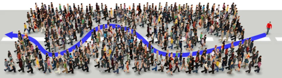
Our results show the improvements in crowd navigation in bidirectional flow as shown in Figure 1, the red pedestrian chose to walk through the moving huge crowd via a clear passageway. This reflects the intelligence in his navigation. Moreover, our approach can automatically exhibit the lane formation phenomenon, which is an important behavior usually emerging in real life, and also the more promising lane changing and overtaking behavior as compared to the previous methods.
Fig. 1. Simulation result generated by our approach. The red-colored pedestrian walks through the huge crowd split by a bent, narrow passageway. At each time step, he observes his surroundings and chooses a comfortable way allowing him to reach to the front area.
2. Previous Work
Computer-aided simulation of the creatures’ behaviors dates back to the work of Reynolds [3] who proposed the model to simulate the movement of the flock of birds. Since then, crowd behaviors have been extensively studied by the researchers in different disciplines, and the plenty of approaches were then developed in an effort to imitate the pedestrian navigation, which will be briefly overviewed in this section.
Global Path Planning (GPP): Dealing with avoiding static obstacles has been much addressed in the robotics literatures where the robot is treated as an intelligent machine capable of sensing the sur-roundings and planning the collision-free trajectories. We refer the reader to the valuable book [4] for the literature review and the useful planning algorithms. Likewise, autonomous pedestrians need to rec-ognize the simulated world, and plan for a route to the destination. The simple way is to discretize the simulated world into the single uniform grid and use the well-known A⋆search algorithm for pathfind-ing, but it is inefficient for a large-scale environment in terms of computation time and memory used, so the multi-resolution grids [5] and the hierarchical pathfinding [6, 7] were introduced to enrich the performance. Owing to the tradeoff between the level of discretization and the performance, using a set of connected graphs to represent the walkable regions is a good choice to compromise between both of them. Many researchers construct such graphs based on different approaches, including the randomized method [8], Delaunay triangulation [9], navigation graph [10], voronoi diagram [11, 12], and medial axis [13, 14, 15, 16, 17]. The graph-based path planners yield a small-sized search space but the queried path, if it exists, is not the shortest one as produced in the grid-based planners. Moreover, the graphs can store additional information of each walkable region, for example, the crowd density [18], to be used as the heuristic value in the traditional graph search algorithms.
trajectories, and parallel-computing capability. With regard to the realism, the example-based method [37, 38, 39, 40], psychology-based method [41, 42], and vision-based method [43] steer the pedestrians, based on the human movement video data, the human psychological factors, and the human visual perception, respectively. Moreover, the continuum crowds [44] and the fluid-like motion [45] can well demonstrate the crowd-level interaction between highly densely-packed crowds, where each individual movement undeniably complies with a group.
Uni- and Bidirectional Crowd Flows: In these situations, the GPP is easily defined due to the simplicity of static obstacle formation, which diverts the researcher interest to the local interaction between pedestrians. Some researchers simulate these circumstances using the lattice-gas model [46, 47] and cellular automata [48, 49, 50] with their own specific rules to determine the lane changing direction on a uniform grid. Although the rules were developed in different ways, the lane changing direction depends on the same attributes, including the crowd density and the walking directions of neighboring pedestrians being in frontal areas. Specifically, these rules will direct the pedestrians to walk on a more comfortable lane such as a low-density lane or a lane having the same-walking-direction pedestrians. By the nature of discretization, limiting pedestrian movement to a discrete set produces unrealistic results. Instead, the counterflow model [51] computes a new desired walking direction, based again on the crowd density and others’ walking directions, enabling pedestrians in any continuous crowd simulators to walk toward a more comfortable area. Moreover, the overtaking analysis based explicitly on the social repulsive forces [52, 53] allows pedestrians to weave their way through a crowd, but the repulsive forces may cancel each other, causing a pedestrian to get stuck into a moving group in front even though walkable pathways are available.
The above-mentioned works determine a new walking direction pointing to a more comfortable lane or area, by considering merely the current state of the neighborings. This does not guarantee the forthcoming movements, and often results in strange-looking behaviors, e.g., confronting the oncoming people, getting stuck into pedestrians in front, or unintentionally being in a dense area, even though other pathways exist. As we point out, the GPP and LCA do not consider the successive walking motion so the awkward behaviors are supposed to emerge. Recently, the navigational system called the Effective Avoidance Combination Strategy (EACS) [54] presented a mid-term motion planning technique, like our MEM, to compute an energy-efficient avoidance path made of successive adaptations. But their resulting path does not guarantee the minimal energy. It depends on the order of collision testing.
In our approach, the presence of MEM produces different behavioral results, comparing to the pre-vious methods using only GPP and LCA. Because in GPP and LCA no successive motions will be taken into account. Although some works exploit crowd density as a heuristic for guiding pedestrian walking, it is limited to some scenarios, for example, the scenario shown in Figure 1. Using crowd density for lane changing direction cannot guide the pedestrian to walk on a narrow passageway. Instead, pedestri-ans in our approach are guided by a collision-free path that yields the minimal energy. Our approach differs from EACS on the aspect that EACS may not consider some feasible paths because some orders of collision testing cannot be reachable so some paths may be skipped. But in our approach the energy-minimal collision-free path is computed from all feasible paths which guarantees that the resulting path yields the global minimum energy.
3. Overview of Our Approach
⃗ di
x y
[image:5.595.229.368.77.194.2]⃗vdes?
Fig. 2. The red pedestrian, who is located at the origin of the reference frame, is desired to walk to-ward the front line, or the red dashed line, with the lowest walking energy expenditure.
for the considered pedestrian. Finally, the LCA will exploit the desired velocity as an input to com-pute the actual one in the sense that the pedestrian attempts to walk along the energy-minimal path simultaneously with preventing collisions with the nearby walkers.
Algorithm 1 shows our simulation loop where the desired walking direction, the desired velocity, and the actual velocity of theith pedestrian were represented byd⃗i,v⃗i,des, and⃗vi,actrespectively. The ComputeDesiredW alkingDirGP P function will be called in every time step to allow the pedestrian to anytime change his mind on the direction towards an exit of the corridor, but in case the direction is fixed, calling it once is enough. Our main contribution is in finding the energy-minimal path in the MEM, which performs through theEnergyM inimalP athM EM(·)function and will be detailed in the next section. The proposed MEM can be seamlessly connected with any previous LCA methods by using the desired velocity as a connector.
Algorithm 1Crowd Simulation in Bidirectional Flow
1: whilesimulatingdo
2: for eachpedestrian ido
3: d⃗i ←ComputeDesiredW alkingDirGP P() 4: ⃗vi,des←EnergyM inimalP athM EM(d⃗i)
5: ⃗vi,act←LocalCollisionAvoidance(⃗vi,des)
6: U pdateP osition(⃗vi,act)
7: end for
8: end while
4. Metabolic-Energy-Minimal Short-Term Path Planning
Our MEM computes the desired velocity⃗vi,desfor each pedestrian on the basis of the principle of least effort and the biomechanical walking energy. The problem we are dealing with was shown in Figure 2. Instead of planning a route to the one end of the corridor, the considered pedestriani, which is depicted by the red circle in Figure 2, will plan its walking path toward the front line being far away from his current position with a distance specified by the user. We assume that the pedestrianiis positioned at the origin of the reference framex-yand only responses to the perceived people in front.
The future position of the perceived people in front will be predicted by two nuanced ways, subject to the distance to the pedestriani. If the distance is below some threshold lth, the future position is
obtained by linearly extrapolating its current velocity, otherwise the projected current velocity onto the desired walking direction d⃗i of the pedestriani. The threshold lth is set to 3.66 meters. This is
in case of bidirectional crowd flow where two pedestrians have a high tendency to meet each other at a future time, if extrapolating the current velocity is used instead, the future position at a large time period may lie outside the corridor and cause no influence on the pedestriani.
The measurement for the walking energy is solely based on the biomechanical study of the real human walking [2] in which the oxygen uptake of a subject walking on a treadmill at varying speeds was recorded, resulting in a mathematical equation that manifests the relationship between the instantaneous metabolic energy expenditure and the walking speed, as shown below.
dE
dt =m(es+ew∥⃗v(t)∥
2) (1)
whereEis the total metabolic energy measured in joules (J),mis the mass measured in kilograms (kg), ⃗v(t) is the velocity at time tmeasured in m/s, es and ew are the constants measured in J/kg/s and Js/kg/m2 respectively, and∥ · ∥ is the Euclidean norm. The constante
sand ew can be viewed as the rates of the energy expended while standing and walking, respectively. These constants are unique for each pedestrian, and for the average human, the constantes is equal to 2.23 J/kg/s while the constant ewis 1.25 Js/kg/m2.
According to Eq. (1), we can compute the total metabolic energy expended by the pedestrianiover arbitrary time period∆tby using the following equation.
E =m
∆t
∫
(es+ew∥v⃗(t)∥2)dt (2) The pedestrianiwill plan its walking path from the current timetcto the unknown future timete(time at which the pedestrianireaches the front line), so∆t=te−tc.
4.1. Constrained Optimization Problem
From the principle of least effort [1], the pedestrian iis supposed to walk with the least amount of energy expenditure. So we compute the desired velocity⃗vi,des(t)for the pedestrianiover time period
[tc, te]such that the total metabolic energyEis minimized: ⃗
vi,des(t) = argmin
⃗ vi(t)∈V
E (3)
whereV is a set of collision-free velocities over time period[tc, te]. Although our objective function is similar to PLEdestrians [56], they are different in purposes. In PLEdestrians, a desired velocity is given and the energy-minimal actual velocity is then computed. Refer to Algorithm 1, PLEdestrians addresses the problem inLocalCollisionAvoidance(·)function.
To define a set of collision-free velocitiesV, the mathematical representation of the front line and the perceived people in front must be well established. We ignore the boundary of the corridor momentarily to examine the energy-minimal walking characteristics of the pedestrianiagainst the perceived people. The front line and thejth perceived people at timetare illustrated by the implicit equationsf(⃗p) = 0 andwj(p, t⃗ ) = 0, respectively, where⃗pis a point(x, y)in the reference frame. The geometric shape of jth perceived people is defined as a circle with the radius(ri+rj), whereri andrj are the radius of the considered pedestrianiandjth preceived people. So
wj(⃗p, t),(rj+ri)2− ∥⃗p−⃗pj(t)∥2 (4) where ⃗pj(t) is the position of the jth perceived people at timet. For the future position of the jth perceived people, we linearly extrapolate its current velocity when the distance to considered pedestrian ibelow the thresholdlth, otherwise the projected one ontod⃗i, so
⃗ pj(t) =
{
⃗
pj(tc) + (t−tc)⃗vj(tc), ∥⃗pj(tc)∥6lth
⃗
pj(tc) + (t−tc)(⃗vj(tc)·d⃗i)d⃗i, otherwise.
With above definition, a velocity⃗vi(t)in a setV must conform to: ˙
⃗
pi(t) =⃗vi(t)
wj(⃗pi(t), t)≤0, j = 1, ..., N f(⃗pi(te)) = 0
(6)
where⃗pi(t)is the position of the pedestrianiat timet, andN is the number of perceived people. The first equation describes the motion of the pedestriani, the second forces the pedestrianinot to collide with the perceived people, and the last one ensures that the pedestrian imust reach the front line at timet=te.
4.2. Metabolic-Energy-Minimal Walking Characteristics
The objective function in Eq.(3) and the constraints in Eq.(6) are investigated to compute⃗vi,des(t)for
t ∈ [tc, te]by using the optimal control theory [57, 58, 59]. The position⃗pi(t)and the velocity⃗vi(t) are respectively the state and the control variable, which characterized by the pure state inequality con-straintswj(⃗pi(t), t) ≤0and the free endpoint conditionf(⃗pi(te)) = 0. The result of the investigation provides us the following equations:
⃗a∗i(t) =− 1 mew
N
∑
j=1
αj(t)(p⃗∗i(t)−p⃗j(t)) (7)
αj(t)wj(⃗p∗i(t), t) = 0 and αj(t)≥0 (8)
⃗v∗i(te) =− 1 2mew
γ∂f
∂⃗p + N
∑
j=1
βj ∂wj
∂⃗p
⃗ p∗i,te
and γ ∈ R (9)
∥⃗vi∗(te)∥=
v u u
tes
ew + 1
mew N
∑
j=1
βj ∂wj
∂t
⃗ p∗i,te
(10)
βjwj(⃗p∗i(te), te) = 0 and βj ≥0 (11) where⃗ai(t)is the acceleration of the pedestrianiat timet, and the asterisk means the variable is com-puted at the optimal point. Eq.(7) and Eq.(8) explain the characteristic of the optimal acceleration that make the pedestrianiexpend the (local) minimal metabolic energy. While Eq.(9) - Eq.(11) tell us about the optimal velocity⃗vi(t)at timet =te (time at which the pedestrianitouches the front linef). For the derivation, please see the appendix A.
The energy-minimal walking characteristics that we can deduce from the equation (7) - (11) are:
Characteristic A.1: For any time period when the pedestrianiwalks without touching any perceived people, he must walk with constant velocity.
Characteristic A.2: For any time period when the pedestrianitouches one of the perceived people; in other words, walks on a circle boundarywj, the relative velocity must be tangent to the circle, and the relative
speed must be constant throughout the time when he is touching.
relative acceleration of the pedestrianiagainst thejth perceived people, and since its direction points to the center, the pedestrianiwill undergo the uniform circular motion on this period, and this results to A.2.
Characteristic B.1: At the timete(when the pedestrianireaches the front linef), if he does not
simul-taneously touch any perceived people, his velocity at that time must be perpendicular to the front linef, and his speed must be equal to√es/ew.
Characteristic B.2: At the timete(when the pedestrianireaches the front linef), if he simultaneously
touches one of the perceived people, his velocity at that time depends on his state at the time before he reaches the front linef.
B.1 and B.2 are the consequence of observing the boundary conditions at timete, as shown in Eq.(9) - Eq.(11). If the pedestrianireaches the front line without touching any perceived people at timete, we obtainwj(⃗p∗i(te), te)<0and thenβj = 0for allj= 1, ..., N in Eq.(11). Therefore, the velocity⃗v∗i(te) in Eq.(9) must be parallel to the gradient off(the normal of the front linef) at the position⃗p∗(te), and its magnitude must be equal to√es/ew as depicted in Eq.(10). This results to B.1. In case he touches one of the perceived people at the timete, sowj(⃗p∗i(te), te) = 0and βj ≥ 0, which gives⃗vi∗(te) the additional dependency on the gradient ofwj (the normal of the circle boundarywj). As the position ⃗
p∗i(t)and the velocity⃗vi∗(t)are continuous for all timet∈[tc, te], and⃗p∗i(te)lies on the circle boundary wj, if the position before he reaches the front linef, denoted by⃗p∗i(te−ϵ)whereϵis a small positive infinitesimal quantity, does not touch any circle boundary, the velocity⃗vi∗(te)will be characterized by A.1. But if⃗p∗i(te−ϵ)lies on a circle boundarywj, A.2 tells us that he is moving in a uniform circular motion at that time and keeps doing this until the timete, so the velocity⃗v∗i(te)will be characterized by A.2.
Characteristic C.1: If there is no perceived people, the pedestrianimust walk straight with the constant speed√es/ewin the direction that is perpendicular to the front linef.
Characteristic C.2: If all perceived people stand still, the pedestrianimust walk with constant speed
√
es/ew throughout the time along the shortest path towards the front line.
C.1 and C.2 explain the walking characteristics in special scenarios. C.1 simply deduces from A.1 and B.1, while C.2 from A.1, A.2, and Eq.(10) with the removal of the time derivatives of allwj. Notice that the walking speed formula√es/ewmatches the most efficient walking speed of the average human studied in the biomechanics [2],√2.23/1.25 = 1.34m/s.
4.3. Near-Global Optimal Solution
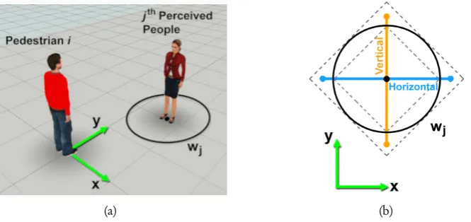
A velocity⃗vi∗(t) that conforms to the above walking characteristics is the local optimal solution to the problem. To find the global one, all possible⃗vi∗(t) need to be given but calculating each velocity ⃗vi∗(t)analytically is not trivial because the transition at a point between A.1 and A.2 is restricted to be continuous. So we present the approximation method by replacing a circlewj with two perpendicular lines, one is parallel to thex-axis of the reference frame, which we called a horizontal line, while the other one is parallel to the y-axis, called a vertical line. The intersection point of these lines is at the center of a circlewj, and the endpoints of each line are at the middle between the corners of the inner and outer rectangles as shown in Figure 3. When the pedestrian i touches thejth perceived people in a period of time (A.2), he will walk between these endpoints instead of the circle boundary. If the endpoints are at the corners of the inner rectangle in Figure 3(b), the pedestrianiwill think that he can walk through two adjacent perceived people, but actually he cannot. If the endpoints are at the corners of the outer rectangle, he will think that he cannot walk through, but actually he can. To compromise these situations, we choose to use the middle points instead.
(a) (b)
Fig. 3. Replacing the circlewjof thejth perceived people (a) with two perpendicular lines (b), called horizontal and vertical lines. While the pedestrianitouches thejth perceived people (A.2), he will walk between the endpoints of lines instead of the circle boundary.
strips. The front linef creates a plane parallel to the time axis, as shown in Figure 4(b).
To find the energy-minimal path, the time axis will be discretized into levels according to the user-defined sampling time∆tsampand the maximum timetmax(Figure 4(c)). At each level, the endpoints of
the horizontal and vertical lines are defined as thecritical points, which perform as the transition points between A.1 and A.2. For the level t = 0, there is only one critical point locating at the origin (⃗0). Instead of naively searching the energy-minimal path from the critical point att = 0to the planef, we use the dynamic programming technique by finding the energy-minimal path starting at the critical points on the top-most level (t=tmax), and then the critical points on the lower level, until the critical
point⃗0is reached.
For each critical point being examined, two types of line segments must be considered, based on the energy-minimal walking characteristics; (1) a√es/ew-slope line segment from the critical point being examined to the closest point on the planef (B.1), and (2) a line segment from the critical point being examined to the critical points on the higher levels (A.1 and A.2). A line segment will be selected as a candidate for constituting the energy-minimal path if no collision with the perceived people occurs, and thanks to each planar strip, the collision detection is very simple by checking only line-plane in-tersection. If the latest-examined line segment and its successor promote the lowest energy, such line segment and its successor will be stored at the critical point being examined, and they will be used as a successor for the critical points on the lower level. If the critical point⃗0is examined and there is no connected sequence of line segments from the critical point⃗0to the plane f, the pedestrian iwill be given the desired velocity√es/ewd⃗i, but if there is a sequence (Figure 4(d)), the desired velocity will be computed from the first line segment (line attached to the critical point⃗0) by the following equation:
⃗vi,des(tc) = (−→cp1− −→cp0)xy/(−→cp1− −→cp0)t (12)
where−→cp1and−→cp0(=⃗0)are the critical points that constitute the first line segment.
4.4. Line Segment Pruning
(a)
t
y
x f
(b)
t
y
x tmax
∆tsamp
f
(c)
t
y
x tmax
∆tsamp
f ⃗
vi∗
[image:10.595.85.510.78.413.2](d)
Fig. 4. Near-global energy-minimal velocity. (a) Pedestrianiperceived two people in front. The fu-ture position of the outside-lth-zone pedestrian is predicted by extrapolating its projected velocity,
and extrapolating the current velocity for the inside one. (b) Horizontal and vertical lines of each per-ceived people generate two perpendicular planar strips, and the front linef creates a plane in space-time coordinate system. (c) The sampling space-time and maximum space-time are defined to discretize the space-time axis into levels to construct critical points. (d) The energy-minimal velocity is computed from⃗vi∗ ob-tained by the dynamic programming technique with the knowledge of the energy-minimal walking characteristics.
in the forward direction (the positive direction of the y-axis), a line segment that points to the negative direction of the y-axis will be pruned.
Moreover, if we found a √es/ew-slope line segment from a critical point being examined to the closest point on the planef, we can discard the line segments between levels since the√es/ew-slope line segment produces the most minimal walking energy from the critical point being examined.
4.5. The Constantes,ew, andtmax
As pedestrians walk at different preferred speed due to their own physiological attributes, for examples, a tall man naturally walks faster than a short one, we handle this diversity in our crowd simulation by setting the constant es and ew for each virtual pedestrian on the assumption that virtual pedestrians expend the same amount of metabolic energy while standing but different while walking. That is:
es = 2.23 ew =es/vpref2
wherevprefis the preferred speed of a virtual pedestrian. The above assumption comes from the situation
when a tall and a short man are at the same position and would like to walk to the same location on the condition that they must reach that location at the same time. The tall man naturally walks faster than the short one by his preferred speed, making the tall man expend the lowest energy, whereas the short one must accelerate himself to pursue the tall man, making the short man walk with higher speed than he prefers, so the short man must spend more energy while walking (ew) for the instantaneous acceleration, and this conduces to Eq.(13).
For the time tmax, it should be equal to or greater than the timete to secure the energy-minimal walking path towards the front linef, however, the timetecannot be known in advance. Nevertheless, tmaxmust be greater than the timetein the situation when the pedestrianiwalks without the perceived people in front (C.1), so the lower bound for tmax is c
√
ew/es, where c is the minimum distance to the front linef. For the upper bound, we define it from the situation when the pedestrianiis closely obstructed by all perceived people which horizontally-packed into a single row, so the pedestrian i must walk to the left or right to avoid the perceived people before walking straight to the front linef. Therefore,
c
√
ew es ≤
tmax≤
(
(largestr
j+ri)N +c
)√ew
es
(14)
where largestr
j is the largest radius among the radii of the perceived people.
5. Results and Discussion
In this section, we will show the results through a set of scenarios, and discuss the efficiency by com-paring with the previous work and the real-world bidirectional crowd flow. We implemented our work in C++ and used OpenGL for visualization on a 64-bit machine with 8GB of RAM, an Intel i7-2600 3.40GHz processor, and with the NVIDIA Geforce GTX 550 Ti. All simulation results are demon-strated in the companion video.
Lane Changing and Overtaking Behavior:The first scenario was shown in Figure 5(a) where the red and yellow pedestrians are walking upward with the desired speed 1.5 m/s and 0.5 m/s respectively, and the three green pedestrians are walking downward with 1.3 m/s. The initial position of the red pedestrian slants a bit to the right side of the yellow one. We compare our method with the social force model, the velocity-based PLEdestrians, and the counterflow model. Since the original social force and the velocity-based models allow the simulated pedestrians to perceive the people in back, causing the people in front to be pushed and/or sidestep, these behaviors should not occur in normal situation of bidirectional crowd flow so we modified by restricting the visual angle to 180 degrees. For our approach, the front linef is set to be a straight liney−cwherecis the planning distance. In this scenario, we set c = 7m and the perception radius is equal toc. Thetmax is set to the halfway between the lower and
upper bound defined in Eq.(14), and the∆tsamp = 0.25s.
(a) Initial (b) Social Force (SFM)
(c) PLEdes-trians
(d) Coun-terflow Model
(e) Ours + SFM
[image:12.595.78.524.75.203.2](f) Ours + PLEdestrians
Fig. 5. From the initial (a), the red pedestrian in the social force model (b), PLEdestrians (c) and Counterflow model (d) walks towards the people in front in an uncomfortable manner by approach-ing to the incomapproach-ing pedestrians although the left area is available. However, the red pedestrian with our MEM ((e) and (f)) can pass through the crowd on the left area, which is collision-free and more comfortable.
The second scenario was shown in Figure 6. The red, blue, and yellow pedestrians are walking upward with desired speed 2.0 m/s, 1.3 m/s, and 0.5 m/s, respectively, and the green ones are walking downward with 1.3 m/s. The front linef,tmax, and∆tsamp for the red pedestrian are identical to the
previous scenario except that c = 10m. The results show that with the social force model (Figure 6(b)) the red pedestrian walked straight towards the group of green people and then was pushed back before escaping to the left, whereas with the PLEdestrians (Figure 6(c)) and the counterflow model (Figure 6(d)), the red pedestrian immediately turned his walking direction to the left when he perceived the green but he afterwards got stuck between the two slow yellow pedestrians. This was due to the opposed influences produced by each yellow pedestrian. If perceiving the people in back is allowed, the two yellow pedestrians will either be pushed or sidestep so that the red one can walk through, which should not be occurred since the adjacent lanes/areas are available.
With our MEM, the red pedestrian walks to the left to avoid the incoming green people, and then overtakes the yellow on the left and finally the blue people on the right, as shown in Figure 6(e) and 6(f). In case the desired speed of the red pedestrian decreases from 2.0 m/s to 1.3 m/s, he still avoids the incoming green people in the same direction as before, but this time he chooses to overtake the yellow on the right, as shown in Figure 6(g), because this path is collision-free, shortest, and energy-minimal for the desired speed 1.3 m/s. On the other hand, when the desired speed increases to 3.0 m/s, he walks straight towards the incoming green people and passes through the crowds via a collision-free gap as shown in Figure 6(h). These behavioral varieties reflect the intelligence in his navigation.
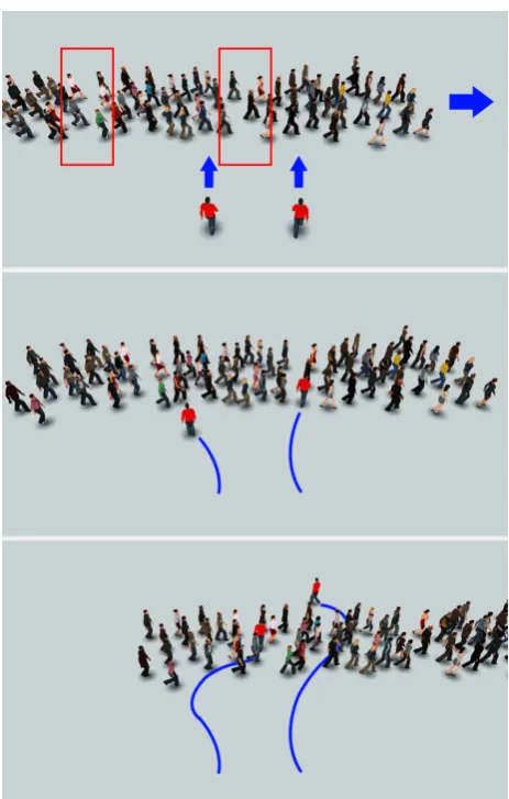
Mimick the Real-World Bidirectional Flow: We also mimicked the real-world bidirectional crowd flow by using our MEM along with the PLEdestrians for LCA, as shown in Figure 7 where the top rows show the image sequence from the video footage of bidirectional crowd flow, and the bottom rows show our mimicking results. Each simulated pedestrian has its own front linef with different planning distancec, and thetmaxand∆tsampare identical to the previous scenarios. After setting and tuning for
c, the simulated pedestrians performed in the same manner as ones in the captured video, which can be seen from the movement of the rectangle-marked pedestrian in Figure 7(a) who runs fast in an upward direction (left column), then slows down for the expected gap (middle column), and finally accelerates to overtake the front people (right column), as well as the movement of the marked pedestrian in Figure 7(b) who walked fast (left column), then overtakes the people in front on the right (middle column), and finally goes through the crowd to the left (right column).
(a) Initial (b) Social Force (SFM) (c) PLEdestrians (d) Counterflow Model
(e) Ours + SFM (f) Ours + PLEdestri-ans
(g) Ours + PLEdes-trians (lower desired speed)
[image:13.595.77.525.74.325.2](h) Ours + PLEdes-trians (higher desired speed)
Fig. 6. From the initial (a), the red pedestrian in the social force model (b) approached to the incom-ing people and then was pushed back by the green pedestrians before escapincom-ing to the left, while in the PLEdestrians (c) and counterflow model (d) the red pedestrian got stuck between two yellow people. However, when equipped with our MEM ((e) - (h)), the red pedestrian can comfortably pass through the crowd on different energy-minimal paths depending on his desired speed.
(a) (b)
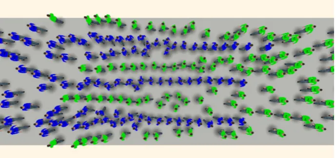
[image:13.595.87.512.414.646.2]Fig. 8. Lane formation simulation from a group of approximately one hundred pedestrians at each one end of the 13-meter-width corridor. The simulated pedestrians are placed randomly in the group and prefer to walk to the opposite side at the desired speed 1.3 m/s.
pedesrians. The simulation result shows that after two groups meet each other around the middle of the corridor, the simulated pedestrians form 7 lanes as shown in Figure 8. If we use longer planning distancec, the lanes are formed faster. The lane formation was made in order to decrease the overall walking energy of the pedestrians, because following the people in front to reach the front line produces lower energy than facing the incoming people.
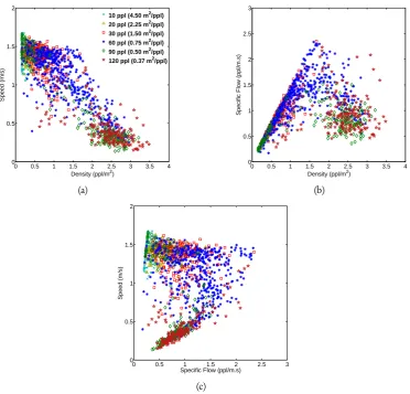
Fundamental Diagrams of Traffic Flow: We also quantitatively examine our approach in bidi-rectional crowd flows through the fundamental diagrams. The simulated pedestrians with the desired speed in a range from 1.3 m/s to 1.7 m/s are placed randomly in the 3m-wide and 15m-long corridor. The number of the pedestrians walking towards the right end of the corridor is equal to one towards the left end. If a pedestrian reaches to the one end, he will show up at the opposite and starts walking again. Thetmaxis set to be halfway between the lower and the upper bound defined in Eq.(14),∆tsamp = 0.25s,
and the planning distancecis 3.66 m for all pedestrians. To obtain the fundamental diagrams, we mea-sure the average speed¯vand crowd densityρin three areas locating at the middle and the ends of the corridor. Givenv¯andρ, the specific flowJsis computed by using hydrodynamic relationJs=ρ¯v.
The flow will be examined at different numbers of pedestrians ranging from 10 to 120 people (equiv-alently to 0.37 m2to 4.50 m2maximum occupation area for a single pedestrian). The crowd density and
the average speed in each area will be measured every frame and averaged over a second interval. After running the simulation, the fundamental diagrams are obtained as shown in Figure 9. Notice that in case of 10 people (4.50 m2/ppl) and 20 people (2.25 m2/ppl), the walking speed of the pedestrians clings
around the desired speed (1.3 m/s - 1.7 m/s) throughout the simulation time, but in case of 30 people (1.50 m2/ppl) it sometimes a bit decreases due to higher population. When the number of pedestrians
increases to 60, or the maximum occupation area per pedestrian reduces to 0.75 m2, the walking speeds
spread widely over the range from approximately 0.3 m/s to 1.6 m/s in a linearly-decreasing pattern as the density increases. This distribution results from dissolving the congestion into the free flow lanes. However, in a highly-dense crowd as demonstrated by the cases of 90 people (0.50 m2/ppl) and 120
peo-ple (0.37 m2/ppl), the free flow lanes are hardly constructed, which makes the pedestrians walk most
of the time at the speeds ranging from approximately 0.15 m/s to 0.5 m/s. Given the specific flow, the relationship between the specific flow and the crowd density is shown in Figure 9(b), while the specific flow and the average speed shown in Figure 9(c). These diagrams have similar trend to the empirical data of bidirectional crowd flow [60] and the traffic flow theory [61].
0 0.5 1 1.5 2 2.5 3 3.5 4 0
0.5 1 1.5 2
Density (ppl/m2)
Speed (m/s)
10 ppl (4.50 m2/ppl) 20 ppl (2.25 m2/ppl) 30 ppl (1.50 m2/ppl) 60 ppl (0.75 m2/ppl) 90 ppl (0.50 m2/ppl)
120 ppl (0.37 m2/ppl)
(a)
0 0.5 1 1.5 2 2.5 3 3.5 4
0 0.5 1 1.5 2 2.5 3
Density (ppl/m2)
Specific Flow (ppl/m.s)
(b)
0 0.5 1 1.5 2 2.5 3
0 0.5 1 1.5 2
Specific Flow (ppl/m.s)
Speed (m/s)
[image:15.595.113.486.76.433.2](c)
Fig. 9. The fundamental diagrams of bidirectional crowd flows generated by our approach.
and 15m-long corridor. The desired speed for each pedestrian is randomly set in a range from 1.3 m/s to 1.7 m/s. At a certain population density, three different setting for the user-defined parameters: (1) c = 3.66m,∆tsamp = 0.25s, (2)c = 3.66m,∆tsamp = 0.50s, and (3)c = 5.00m,∆tsamp = 0.25s,
will be used for the quantitative comparison.
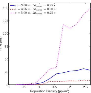
After measuring at 12 population densities ranging from 0.2 ppl/m2 to 2.66 ppl/m2, the trend of
the average computation times has been produced as shown in Figure 10. It is not surprising that at a certain population density the average computation time increases as the planning distancecincreases and/or the sampling time∆tsampdecreases because the increase ofcand/or the decrease of∆tsampcause
the higher number of critical points. However, when observing their margins, the average computation times in all three settings are not significantly different at the population densities below 1 ppl/m2, but
dramatically expand at the higher population densities. If the long planning distancecwith the precise time sampling∆tsampis used, the computation time must be expensive in high-density crowds. This is
the limitation of our approach if the real-time computation for the dense crowds is required.
0 0.5 1 1.5 2 2.5 0
25 50 75 100 125 150
Population Density (ppl/m2)
Time (ms)
c= 3.66 m, ∆tsamp= 0.25 s
c= 3.66 m, ∆t
samp= 0.50 s
c= 5.00 m, ∆t
[image:16.595.206.392.77.267.2]samp= 0.25 s
Fig. 10. The average computation time of our approach in three different setting at different popula-tion densities.
that are marked with the red-colored rectangles.
In the other example as shown in Figure 12, pedestrians with the desired speeds ranging from 1.0 m/s to 1.4 m/s are placed at two circle boundaries (Figure 12(a)), and the goal position for each pedestrian is located at the opposite. At frame 725 (∼12 seconds), the pedestrians in the social force model (Figure 12(b)), PLEdestrians (Figure 12(c)), and ORCA (Figure 12(d)) are mostly packed at the center, but when equipped with our MEM, the pedestrians are scattered and some of them almost reach to their own goal positions. This is because the pedestrians with our MEM respond to the others in an early time of simulation by planning the collision-free, comfortable paths towards their goals.
6. Conclusion and Future Work
The short-term path planning based on the principle of least effort with the energy calculation using the metabolic energy equation of the real human walking was proposed. The technique can be seam-lessly integrated with previous local collision avoidance methods, which allows the virtual pedestrians in bidirectional crowd flows to walk on energy-minimal paths. This results in more promising overtak-ing behavior and more reasonable lane changovertak-ing direction, and in addition can achieve lane formation phenomenon and also generate the same trend of the fundamental diagrams as ones in the empirical data and the traffic flow theory. To obtain energy-minimal paths, we formulate the problem as the optimiza-tion problem and employ the optimal control theory with the dynamic programming as a solver. The algorithm can perform well in low-to-medium population density but yields the expensive computation in dense crowds. Also, our approach can be used for multi-directional crowd simulation with a little modification. For the future work, we plan to reduce the computational burden by finding the heuristic to determine when our MEM should operate, and the efficient method for adaptive planning distance c.
Acknowledgements
Fig. 11. Image sequence (from top to bottom) of two red pedestrians walking upward against a flow of crowds by using our approach. The red pedestrians can walk through the flow via the two tunnels marked by the red-colored rectangles.
(a) Initial (b) Social Force (SFM) (c) PLEdestrians (d) Optimal Reciprocal Col-lision Avoidance (ORCA)
(e) Ours + SFM (f) Ours + PLEdestrians (g) Ours + ORCA
[image:17.595.77.523.507.702.2]Appendix A Derivation of Energy-Minimal Walking Characteristics
A.1 Optimization Problem
Our optimization problem begins with minimizing the objective function in the integral form as shown in the following equation:
E =
∫ t1
t0
g(t, ⃗p(t), ⃗v(t))dt, (15)
where ⃗p ∈ Rm and⃗v ∈ Rn are called the state and control variables, respectively, andg(·)is a real-valued function. When the values of the control variables⃗vchange, the values of the state variables ⃗p will be changed simultaneously by this differential equation:
˙ ⃗
p(t) =⃗h(t, ⃗p(t), ⃗v(t)), (16)
where⃗h(·) is arbitrary vector function that has the same dimension as⃗p. The state ⃗p(t) is also con-strained by theN inequality equations:
wj(⃗p(t), t)≤0, j= 1, ..., N (17) for allt∈[t0, t1], and one endpoint constraint:
f(⃗p(t1)) = 0. (18)
The function wj andf are the real-valued functions. We assume that all functions are continuously differentiable with respect to their own independent arguments. Notice that the control function⃗v(t) influences the functionalEdirectly by its own values and indirectly by its impact on the state function ⃗
p(t)in Eq.(16). Moreover, in our problem, the initial point of the state⃗p(t)is fixed in both space and time, and can be computed in advance. That is:
t0and⃗p(t0)are fixed to the known values.
A.2 Necessary Conditions for Optimality
To find the optimal trajectory (t,⃗p∗(t),⃗v∗(t)), we first eliminate Eq.(16) by appending it into the func-tionalE with the Lagrange multiplier vector function⃗λ(t), which results in:
E =
∫ t1
t0
g(t, ⃗p(t), ⃗v(t)) +⃗λ(t)·(⃗h(t, ⃗p(t), ⃗v(t))−p⃗˙(t))dt, (19)
where the Lagrange multiplier⃗λ(t) ∈ Rm can be arbitrary vector function. Then, we expand the product term and apply the integration by parts, so Eq.(19) turns out to be:
E=
∫ t1
t0 (
g+⃗λ·⃗h+⃗λ˙ ·⃗p
)
dt+⃗λ(t0)·⃗p(t0)−⃗λ(t1)·⃗p(t1), (20)
Note that we discard the arguments of the functions in the integral just because of the limited space and for the clear explanation. Please remember that such functions still depend on their own independent variables that are previously displayed. We assume that the optimal trajectory (t,p⃗∗(t),⃗v∗(t)) over time period[t0, t1]produces the minimum functionalE∗within some neighborhoodsE, so from Eq.(20) we
obtain:
E∗ =
∫ t1
t0 (
g∗+⃗λ·⃗h∗+⃗λ˙ ·⃗p∗
)
dt+⃗λ(t0)·⃗p∗(t0)−⃗λ(t1)·⃗p∗(t1), (21)
For the neighborhoods of (t,⃗p∗(t),⃗v∗(t)), if trajectories (t, ⃗p(t),⃗v(t)) fort ∈ [t0, t1 +δt1]are its
neighborhoods, they must produce higher or equal functionalEto the minimum functionalE∗. Note that the state at the endpoint in our case is free in both space and time, so the time of the endpoint of neighboring trajectories can be shifted and this is the reason why the upperbound must bet1+δt1, where
δt1is a small infinitesimal quantity. From Eq.(19), the functionalEproduced by the neighborhoods (t,
⃗
p(t),⃗v(t)) can be computed by:
E =
∫ t1+δt1
t0
(
g+⃗λ·⃗h−⃗λ·⃗p˙
)
dt. (22)
Rewrite Eq.(22) by splitting the integral at timet1into two separate terms, so
E =
∫ t1
t0 (
g+⃗λ·⃗h−⃗λ·⃗p˙
)
dt+
∫ t1+δt1
t1
(
g+⃗λ·⃗h−⃗λ·⃗p˙
)
dt. (23)
The first integral term on the right side of Eq.(23) is the same form as one in Eq.(19), so it can be replaced with the right side of Eq.(20). Therefore,
E=
∫ t1
t0 (
g+⃗λ·⃗h+⃗λ˙ ·⃗p
)
dt+⃗λ(t0)·⃗p(t0)−⃗λ(t1)·⃗p(t1)
+
∫ t1+δt1
t1 (
g+⃗λ·⃗h−⃗λ·⃗p˙
)
dt.
(24)
Consider the last integral term in Eq.(24), it can be approximated by:
∫ t1+δt1
t1
(
g+⃗λ·⃗h−⃗λ·⃗p˙
)
dt≈
(
g+⃗λ·⃗h−⃗λ·⃗p˙) t1
δt1
=g|t=t1δt1 ≈
(
g∗+∂g ∗
∂⃗p ·∆⃗p+ ∂g∗
∂⃗v ·∆⃗v+R ∗
2
)
t=t1
δt1
≈g∗|t=t1δt1
(25)
where∆⃗p(t) =⃗p(t)−⃗p∗(t),∆⃗v(t) =⃗v(t)−⃗v∗(t), andR∗2is the remainder. The second line in Eq.(25) is from eliminating the last two terms in the first line. This was due to the equality constraint specified in Eq.(16). The third line results from applying the Taylor series expansion to the functiong about the optimal trajectory (t,⃗p∗(t),⃗v∗(t)). The term∆⃗pδt1,∆⃗vδt1, andR∗2δt1 are very small, so they are
eliminated, and the approximation ends in the last line. Therefore, Eq.(24) becomes:
E=
∫ t1
t0 (
g+⃗λ·⃗h+⃗λ˙ ·⃗p
)
dt+⃗λ(t0)·⃗p(t0)−⃗λ(t1)·⃗p(t1)
+g∗|t=t1δt1
(26)
Since the functionalE∗is a local minima within some neighborhoodE, which is expressed by Eq.(26), so we get
E−E∗≥0. (27)
ConsiderE−E∗from Eq.(21) and Eq.(26),
E−E∗,
∫ t1
t0 (
(g−g∗) +⃗λ·(⃗h−⃗h∗) +⃗λ˙ ·(⃗p−⃗p∗)
)
dt
+⃗λ(t0)·
(
⃗
p(t0)−⃗p∗(t0)
)
−⃗λ(t1)·
(
⃗
p(t1)−⃗p∗(t1)
)
Then, we use the Taylor series expansion on the termsg−g∗and⃗h−⃗h∗, and change⃗p−p⃗∗to∆⃗p.
E−E∗ ,
∫ t1
t0 {(
∂g∗
∂⃗p ·∆⃗p+ ∂g∗
∂⃗v ·∆⃗v
) + m ∑ i=1 λi (
∂h∗i
∂⃗p ·∆⃗p+ ∂h∗i
∂⃗v ·∆⃗v
)
+⃗λ˙ ·∆⃗p
}
dt
+⃗λ(t0)·∆⃗p(t0)−⃗λ(t1)·∆⃗p(t1)
+g∗|t=t1δt1,
(28)
whereλiis theith component of the Lagrange multiplier vector function⃗λ, andhiis theith component of the vector function⃗h. As the state at initial point, the state at timet0, in our case is fixed in both
space and time, so∆⃗p(t0) = 0, and Eq.(28) becomes:
E−E∗ ,
∫ t1
t0 {(
∂g∗
∂⃗p ·∆⃗p+ ∂g∗
∂⃗v ·∆⃗v
) + m ∑ i=1 λi (
∂h∗i
∂⃗p ·∆⃗p+ ∂h∗i
∂⃗v ·∆⃗v
)
+⃗λ˙ ·∆⃗p
}
dt
−⃗λ(t1)·∆p⃗(t1) +g∗|t=t
1δt1.
(29)
Letδ⃗p1be the difference between the endpoint of the optimal state⃗p∗, which ends at the timet1, and the
endpoint of the neighborhood⃗p, which ends at the timet1+δt1. Specifically,δ⃗p1=p⃗(t1+δt1)−⃗p∗(t1).
So∆p⃗(t1)can be approximated by:
∆p⃗(t1)≈δ⃗p1−p⃗˙∗(t1)δt1. (30)
Replacing it in Eq.(29) results in:
E−E∗ ,
∫ t1
t0 {(
∂g∗
∂⃗p ·∆⃗p+ ∂g∗
∂⃗v ·∆⃗v
) + m ∑ i=1 λi (
∂h∗i
∂⃗p ·∆⃗p+ ∂h∗i
∂⃗v ·∆⃗v
)
+⃗λ˙ ·∆⃗p
}
dt
+
(
g∗|t=t1+⃗λ(t1)·⃗p˙∗(t1) )
δt1−⃗λ(t1)·δ⃗p1.
(31)
Rearrange terms in the integrand in Eq.(31), so we get:
E−E∗ ,
∫ t1
t0 {(
∂g∗ ∂⃗p +
m
∑
i=1
λi ∂h∗i
∂⃗p + ˙ ⃗λ
) ·∆⃗p
+
(
∂g∗ ∂⃗v +
m
∑
i=1
λi ∂h∗i
∂⃗v
) ·∆⃗v
}
dt
+
(
g∗|t=t1 +⃗λ(t1)·⃗p˙∗(t1) )
δt1−⃗λ(t1)·δ⃗p1.
(32)
LetH(t, ⃗p(t), ⃗v(t), ⃗λ(t)) =g+⃗λ·⃗h, which is called the Hamiltonian. So Eq.(32) turns out to be:
E−E∗ ,
∫ t1
t0 {(
∂H∗ ∂⃗p +
˙ ⃗ λ
) ·∆p⃗+
(
∂H∗ ∂⃗v
) ·∆⃗v
}
dt
+
( H∗|t=t1
)
δt1−⃗λ(t1)·δ⃗p1.
From Eq.(27) and Eq.(33), the optimal trajectory(t, ⃗p∗, ⃗v∗)which produces the local minimum func-tionalE∗ must satisfy the following equation:
∫ t1
t0 {(
∂H∗ ∂⃗p +
˙ ⃗λ
) ·∆⃗p+
(
∂H∗ ∂⃗v
) ·∆⃗v
}
dt
+
( H∗|
t=t1 )
δt1−⃗λ(t1)·δ⃗p1 ≥0.
(34)
The optimal trajectory (t, ⃗p∗, ⃗v∗) yields the local minimum E∗ over all admissible neighborhoods (t, ⃗p, ⃗v), andsomeneighborhoods(t, ⃗p, ⃗v)could have the same endpoint in both space and time as the endpoint of the optimal trajectory(t, ⃗p∗, ⃗v∗), that isδt1 = 0andδ⃗p1= 0, which turns Eq.(34) into
∫ t1
t0 {(
∂H∗ ∂⃗p +
˙ ⃗λ
)
·∆⃗p+
(
∂H∗ ∂⃗v
) ·∆⃗v
}
dt≥0. (35)
So the optimal trajectory(t, ⃗p∗(t), ⃗v∗(t))must satisfy
(
∂H∗ ∂⃗p +
˙ ⃗λ
) ·∆⃗p+
(
∂H∗ ∂⃗v
)
·∆⃗v≥0, (36)
for allt∈[t0, t1]. Back to theNinequality constraints in Eq.(17). We call the constraintwjisinactiveat timet, ifwj(⃗p(t), t)<0; otherwise,activeat timet. If the optimal state⃗p∗(t)makes thejth constraint wjinactive at a certain timet, sowj(⃗p∗(t), t)<0. However, for any neighborhood⃗p(t), it must satisfy Eq.(17), sowj(⃗p(t), t)≤0. This conduces to:
wj(⃗p(t), t) {>,=,or <} wj(⃗p∗(t), t)
which places no restriction on ∆⃗p(t). On the other hand, if the optimal state ⃗p∗(t) makes the jth constraintwj active at a certain timet, sowj(⃗p∗(t), t) = 0, and, as before, the neighborhood⃗p(t)must satisfywj(⃗p(t), t)≤0. This conduces to:
wj(⃗p(t), t)≤wj(p⃗∗(t), t) and results in the restriction on∆p⃗(t)as shown below:
∂wj∗
∂⃗p ·∆⃗p≤0. (37)
In case the optimal state⃗p∗(t)makesallconstraintswjinactiveat a certain timet, so∆⃗p(t)will not be constrained by anywj. This leads to any possibilities of values of∆⃗pat timet. Likewise, the control ⃗v(t) is also arbitrary, leading to arbitrary∆⃗v as well. Therefore, to satisfy Eq.(36) when∆⃗p(t) and ∆⃗v(t)can be arbitrary, the terms in the parentheses must be zero:
∂H∗ ∂⃗p +
˙ ⃗
λ= 0 and ∂H∗
∂⃗v = 0. (38)
Eq.(38) expresses the characteristics of the optimal state ⃗p∗(t) and optimal control⃗v∗(t) in a certain time period when all inequality constraints are inactive. In case the optimal state⃗p∗(t)makessome/all
constraintswj active. All activewj must place the restriction on∆⃗p(t), as shown in Eq.(37). So ∂wj∗
where Atis a set of indices of the active constraints at timet. To satisfy Eq.(36) when∆p⃗(t)is con-strained by Eq.(39), the Farkas’s lemma, described in the appendix B, is then employed. This results in:
∂H∗ ∂⃗p +
˙ ⃗ λ+ ∑
j∈At
αj(t) ∂w∗j
∂⃗p = 0 and ∂H∗
∂⃗v = 0, (40)
where αj(t) ≥ 0 for all j ∈ At. Eq.(40) expresses the characteristics of the optimal state ⃗p∗(t) and optimal control⃗v∗(t)in a certain time period when some/all inequality constraints are active.
Notice from Eq.(38) and Eq.(40) that if an inequality constraint becomes active by the optimal state ⃗
p∗, the termαj∂w∗j/∂⃗pwill be added. So we generalize this by raising the additional equation shown below:
αj(t)wj(⃗p∗(t), t) = 0, j= 1, ..., N. In summary, the optimal trajectory(t, ⃗p∗(t), ⃗v∗(t))must satisfy:
˙
⃗λ+∂L∗ ∂⃗p = 0 ∂L∗
∂⃗v = 0
αj(t)wj(⃗p∗(t), t) = 0, j= 1, ..., N αj(t)≥0, j= 1, ..., N
⃗λ(t)∈ Rm,
(41)
for allt∈[t0, t1], whereLis called the Lagrangian and equals to:
L(t, ⃗p(t), ⃗v(t), ⃗λ(t), α1(t), ..., αN(t)) =H+
N
∑
j=1
αj(t)wj(⃗p(t), t).
So far we completely investigate the characteristics of the optimal trajectory(t, ⃗p∗, ⃗v∗)against the neigh-borhoods(t, ⃗p, ⃗v)that have the same endpoint in both space and time as one of the optimal trajectory. Now it is time to investigate the characteristics of the optimal trajectory(t, ⃗p∗, ⃗v∗) against the neigh-borhoods (t, ⃗p, ⃗v) that have different endpoint to one of the optimal trajectory. That isδt1 ̸= 0and
δ⃗p1 ̸= 0. Do not forget that Eq.(34) must hold for the optimal trajectory(t, ⃗p∗, ⃗v∗), and because Eq.(35)
holds in the previous investigation, so Eq.(34) turns out to be:
( H∗|t=t1
)
δt1−⃗λ(t1)·δ⃗p1≥0. (42)
However, the endpoints are constrained by Eq.(18), which yields:
f(⃗p∗(t1)) = 0 and f(⃗p(t1+δt1)) = 0.
Recall that the optimal state⃗p∗and the neighborhood⃗pare assumed to end at the timet1andt1+δt1,
respectively. Because of⃗p(t1+δt1) =⃗p∗(t1) +δ⃗p1, so we get:
f(⃗p∗(t1)) = 0 and f(⃗p∗(t1) +δ⃗p1) = 0.
Using the Taylor series expansion to above equations yields the following constraint towardsδ⃗p1:
(
∂f∗ ∂⃗p
t=t1 )
Eq.(43) can be added into Eq.(42) without loss of generality by multiplying with the real-valued constant variableγ, and then adding into Eq.(42). Therefore, the optimal trajectory(t, ⃗p∗, ⃗v∗)must satisfy:
( H∗|
t=t1 )
δt1+
( γ∂f ∗ ∂⃗p
t=t1
−⃗λ(t1)
)
·δ⃗p1 ≥0, (44)
where γ ∈ R and can be arbitrary real value. However, the endpoints are not constrained by only Eq.(18) but Eq.(17) as well. If the endpoint of the optimal statep⃗∗makeswjinactive, sowj(⃗p∗(t1), t1)<
0, and again,wj(⃗p(t1 +δt1), t1+δt1)≤ 0must hold for the endpoint of the neighborhood⃗p, which
results in:
wj(⃗p(t1+δt1), t1+δt1) {>,=, or <} wj(p⃗∗(t1), t1).
The above equation places no restriction onδ⃗p1. On the one hand, if it makeswjactive, sowj(⃗p∗(t1), t1) =
0, and
wj(⃗p(t1+δt1), t1+δt1)≤wj(⃗p∗(t1), t1).
The above equation places the restriction on bothδ⃗p1 andδt1, as shown below:
(∂w∗
j ∂t
t=t1 )
δt1+
(∂w∗
j ∂⃗p
t=t1 )
·δ⃗p1 ≤0. (45)
In case the endpoint of the optimal state⃗p∗(t)makesallconstraintswj inactive,δ⃗p1 and also δt1
can be arbitrary values, and in order to satisfy Eq.(44), the terms in the parentheses must be zero:
H∗|t=t1 = 0 and ( γ∂f ∗ ∂⃗p
t=t1 )
−⃗λ(t1) = 0. (46)
Eq.(46) expresses the characteristics of the optimal state⃗p∗(t)and optimal control⃗v∗(t)at the timet1
when all inequality constraints are inactive.
In case the endpoint of the optimal state⃗p∗(t)makessome/allconstraintswj active. All activewj must place the restriction on bothδ⃗p1 andδt1, as shown in Eq.(45). So
(∂w∗
j ∂t
t=t1 )
δt1+
(∂w∗
j ∂⃗p
t=t1 )
·δ⃗p1≤0, j∈ At1. (47)
To satisfy Eq.(44) whenδ⃗p1 andδt1 are constrained by Eq.(47), the Farkas’s lemma is employed again,
which results in:
H∗|t=t1 + ∑
j∈At1
βj ∂w∗j
∂t
t=t1
= 0,
( γ∂f ∗ ∂⃗p
t=t1 )
−⃗λ(t1) + ∑ j∈At1
βj ∂w∗j
∂⃗p
t=t1
= 0,
(48)
whereβj ≥0for allj ∈ At1. Eq.(48) expresses the characteristics of the optimal state⃗p∗(t)and optimal
control⃗v∗(t)at the timet1when some/all inequality constraints are active.
Notice from Eq.(46) and Eq.(48) that if an inequality constraint becomes active at time t1 by the
optimal statep⃗∗, the termβj∂w∗j/∂tand βj∂wj∗/∂⃗p will be added. We generalize this by raising the additional equation shown below: