A nonstandard higher-order variational model to speckle noise removal and thin-structure detection

A nonstandard higher-order variational model to speckle noise

removal and thin-structure detection

Hamdi Houichet

_{Anis Theljani}

_{Maher Moakher}

_{Badreddine Rjaibi}

June 19, 2017

Abstract

In this work, we propose a multiscale approach for a nonstandard higher-order PDE based on thep(·)-Kirchhoff energy. First, we consider a topological gradient approach for a semi-linear case in order to detect important object of image. Then, we consider a fully nonlinear p(·)-Kirchhoff equation with variables exponent functions that are chosen adaptively based on the map furnished by the topological gradient in order to preserve important features of the image. Then, we consider the split Bregman method for the numerical implementation of our proposed model. We compare our model with other classical variational approaches such that the TVL and biharmonic restoration models. Finally, we present some numerical results to illustrate the effectiveness of our approach.

Keywords: Inverse problems, regularization procedures, p(·)-Kirchhoff, topological gradient, split Bregman.

1

Introduction

Image restoration is a fundamental task in image processing and it arises in diverse fields (geophysics, optics, medical imaging, etc). In this work, we are interested in the restoration of images highly corrupted with multiplicative noise. It is a challenging task in various fields and particularly in ultrasound medical imaging. The reason is that ultrasound images are strongly influenced by the quality of data usually corrupted with Rayleigh-distributed multiplicative noise. The latter is so-called speckle noise [30, 31, 34] and usually affects image analysis methods by making important features hard to detect. We aim to reconstruct an image u: Ω→Rfrom an observed one f : Ω⊂R2_{→Rwhich is} degraded and contaminated by noise. The degradation model that we consider is the following:

f =u+g(u)η, (1)

whereη: Ω→Ris a positive function that follows the Rayleigh-distribution. The functiong(·) encodes the noise type in such a way that g(u) _≡ 1 in the case of additive Gaussian noise, i.e., f = u+n, and g(u) = √u in the case of speckle (multiplicative) noise. The reconstruction problem based on model (1) is an ill-posed inverse problem and thus regularization techniques are needed to overcome ill-posedness. Generally, the regularization technique turns the reconstruction problem based on model (1) into a well-posed optimization one where the energy to be minimized is the sum of a regularization

∗_{University of Tunis El Manar, National Engineering School at Tunis, Laboratory for Mathematical and Numerical}

Modeling in Engineering Science, B.P. 37, 1002 Tunis-Belv´ed`ere, Tunisia. Emails: [email protected](H. Houichet),[email protected](M. Moakher) [email protected](B. Rjaibi).

†_{Liverpool Centre for Mathematics in Healthcare, Department of Mathematical Sciences, University of Liverpool,}

Liverpool, UK. Email: [email protected].

term (mostly a semi-norm of a functional space fixed a priori) and a data fitting term. In general, the well-posed minimization problem has the following form:

min {u>0;u∈H}

(

J(u) :=J(u) +λ

Z

Ω

f₋u

g(u)

2 dx

)

, (2)

The first part in energyJ(·) is a regularization term, the second one is the fitting term,λis a positive weight which controls the trade-off between them and _H is a space of the solution.

The main issue is how to choose the “best” regularization term which can selectively smooth a noisy image without losing significant features such as edges and thin structures. In various recent works [9, 10, 37], higher-order derivatives have been used to damp oscillations and to avoid stair-casing effect of second order derivatives. In [13], Chan, Marquina and Mulet used the following regularizer:

JCM M(u) =

Z

Ω

|∇u_|+ (∆u) 2

|∇u_|3

dx,

where ∇ and ∆ denote the gradient and the Laplace operators, respectively. Another prominent regularizer using higher-order derivatives was proposed by You-Kaveh [44] by considering:

JY K(u) =

Z

Ω

f(_|∆u_|) dx,

which, when f(s) = s, leads to a nonlinear (TV-like) higher-order PDE and when f(s) = s2 to the biharmonic equation -plenty regularization. In this work, we consider a new regularization term defined by a regularizer which is a compromise between the extreme cases f(s) =s and f(s) = s2. More precisely, we consider the following regularizer:

Jp,q(u) =α

Z

Ω 1

p(x)|∆u|

p(x)_dx+βZ

Ω 1

q(x)|∇u|

q(x)_{dx, (3)}

where the functions p(_·) andq(_·) are defined on Ω and satisfy 1< p(_·), q(_·)_≤2. Nonstandard PDEs with variable exponentp(.), specially for thep-Laplace equation, were considered in several works (see [8, 22, 33]). A lot of research recently studied partial differential equations and variational problems with p(·)-growth conditions which arise in electro-rheological fluids [38], elasticity theory [45] and image processing [14, 28, 32].

The smoothness propriety in these nonstandard PDEs is driven by the variables exponent p(·) and q(_·). The approach that we propose automatically balances between L1_{-Lalpacian (respectively}

L1_{-gradient) and L}2_{-Laplacian (respectively L}2_{-gradient) regularization effects. Thus, by giving the} variable exponentp(·) andq(·) the possibility to take values between 1 and 2 we allow to slow diffusion near edges, and enhance diffusion in smooth regions. This choice avoids over smoothing and stair-casing artifact effects of L2_{- and L}1_{-regularization. However, a common question is how to choose} the values of the exponents p(_·) andq(_·)? A classical idea is to make an adaptive choice forp(_·) and

This paper is organized as follows. In Section 2, we fix notations and recall useful results for the generalized Lebesgue/Sobolev spaces. In Section 3, we prove, by standard variational techniques, the existence and uniqueness of the minimizer of the energy functional (2). In Section 4, we give the formula of the topological gradient for p(_·)_≡q(_·)_≡2. In section 5, we present the adaptive algorithm and we present the split Bregman scheme for the restoration process. Finally, in Section 6, we treat some numerical examples to test its efficiency and robustness.

2

Preliminaries and notations

Before going further, we recall some useful definitions and results about the variable-exponent gener-alized Lebesgue and Sobolev spacesLp(·)_{(Ω) and W}k,p(·)_{(Ω). For more details, we refer the reader to} [15, 17, 18, 20, 21]. For a bounded Lipschitz open set Ω_⊂RN _{with sufficiently smooth boundary∂Ω,} we define the variable-exponent generalized Lebesgue spaceLp(·)(Ω) as follows:

Lp(·)(Ω) :=u: Ω_→Rmeasurable and

Z

Ω|

u(x)_|p(x)dx <_∞ ,

where p(_·)_∈C(Ω) be a measurable function, called variable exponent on Ω and satisfy the following condition:

1< p−:= inf

x∈Ω≤p(x)≤p

+_{:= sup}

x∈Ω

p(x)_≤2. (4)

Lp(·)(Ω) is a normed linear space equipped with the Luxemburg norm:

kukLp(·) = inf

% >0 :

Z

Ω

u(_%x)p(x)dx≤1

.

The Sobolev space with variable exponentWk,p(·)(Ω) is defined as:

Wk,p(·)(Ω) =u_∈Lp(·)(Ω) :Dξu_∈Lp(·)(Ω),_|ξ_{| ≤}k ,

where Dξu = ∂|ξ| ∂xα1

1 ∂x ξ2 2 ...∂xξNN

u with ξ = (ξ1, . . . , ξN) is a multi-index and |ξ| = PNi=1ξi. The space

Wk,p(·)(Ω), is equipped with the norm:

ku_kk,p(·):= X |ξ|≤k

||Dξu_||Lp(·).

Both (Lp(·)_{(Ω),|| · ||}

Lp(·)) and (Wk,p(·)(Ω),|| · ||_k,p(·)) are separable, reflexive and uniformly convex Banach spaces [21].

Lemma 2.1 [15] (Generalized Poincar´e’s inequality). If Ω is a Lipschitz domain, then, there

exists a constant C >0 such that for all u∈W1,p(·)(Ω):

u− _|Ω1_| Z Ω u dx

Lp(·) ≤

C_k∇u_kLp(·).

Remark 2.1 We consider the following space X = _{u_∈W2,p(·)_(Ω)|∂u

∂n = 0}. The norm kuk2,p(·) is equivalent to the norm_ku_kX =k∆ukLp(·) in the spacesW2,p(·)(Ω)andX. Moreover,(W2,p(·)(Ω);k·kX) and (X;_{k · k}X) are Banach, separable and reflexive spaces.

We consider the space ˜W1,p(·)(Ω) =_{u_∈W1,p(·)(Ω);R_Ω(u₋f)dx= 0_}, and the potentials Jp(_·) =

R

Ωp(1x)|∆· |p(x)dxandJq(·) =

R

Proposition 2.2 For sequences (un)n∈W2,p(·)(Ω) and(vn)n∈W˜1,q(·)(Ω), as n→ ∞ we have:

(a) _kunk2,p(·)→ ∞ ⇔Jp(un)→ ∞.

(b) kvnk_W1,q(·) → ∞ ⇔Jq(vn)→ ∞.

Proof: The proof of this proposition is similar to the proof of Theorem 1.3 in [21].

3

Mathematical formulation of the problem

Let p(_·), q(_·) _∈C(Ω) such that these two functions are not related to each other. For our purpose, they just have to satisfy (4). Adapted to our specific problem here, we introduce the working space

Hp(·) _by:

Hp(·)(Ω) =X_∩W1,q(·)(Ω),

which can be equipped with the norm_{|| · ||}=_k∆_{· kL}p(·)+k∇ · k_Lq(·).

In this paper, we discuss the image restoration problem, using model (2), based on the minimization of the following energy:

J(u) =

Jp,q(u) +λ

Z

Ω

W(u, f) dx

, (5)

whereW is the locally Lipschitz continuous function defined by:

W(s, z) :=

z−s

g(s)

2

∀s, z >0.

For any s >0,W(s,_·) is a strict convex function. Moreover, the first-derivative ofW with respect to

s is

∂W

∂s (s, z) =φ(s)(s−z) where φ(s) =

g(s) + (s−z)g0(s)

g(s)3

is positive when 0<infz _≤s_≤supz.

Moreover, letm, M >0 such thatm_≤s_≤M, the following inequality hold

∂W

∂s (m, z)≤0 and ∂W

∂s (M, z)≥0. (6)

For brevity, we sometimes write W(_·) forW(_·, f) andDuW(·, f) forW0(·, f).

3.1

Existence and uniqueness of solution

In the sequel, we establish the well-posedness of the following minimization problem:

min

u∈Hp(·)_(Ω){J(u)|

Z

Ω

(f₋u)dx= 0_}. (7)

Proposition 3.1 The minimization problem (7)admits a unique minimizeruin_Hp(·)_{(Ω). Moreover,}

we have

0<inf

Proof: First, it easy to see that the energyJ(·) is strictly convex and weakly lower semi-continuous in the space Hp(·)_{(Ω). Let us consider a minimizing sequence (u}

n)n⊂H(Ω) :={u >0, u∈ Hp(·)(Ω)} of_J(_·), i.e.,

J(un) −→

n→∞u∈Hinfp(·)_(Ω)J(u).

We denote by m := infΩf and M := supΩf and let (vn)n ⊂ H(Ω) be the sequence defined by

vn= min(un, M) and setD={x∈Ω; un(x)≥M}. Since on Ω\D we haveun=vn, it follows that

J(vn)− J(un) =−α

Z

D 1

p(x)

|∆vn|p(x)+|∆un|p(x)

dx + Z D

(W(M)−W(un)) dx

−β

Z

D 1

p(x)

|∇vn|q(x)− |∇un|q(x)

dx

. (9)

Using the convex property of W and the second inequality in (6), we can write:

Z

D

(W(M)−W(un)) dx≤ −

Z

D

DuW(M)(M−un)≤0.

It follows that J(vn)≤ J(un) and (vn)n is also a minimizing sequence satisfying vn≤M. The same analysis goes for wn = max(un, m) and we also obtain that (wn)n satisfying m≤ wn. Therefore, we can assume, without restriction, that m _≤ un ≤ M. In addition, since R_Ω(u−f) dx = 0, from the previous inequality, Proposition 2.2 and the Poincar´e’s inequality, we easily get the sequence (un)n is uniformly bounded in Hp(·)_{(Ω). Thus, there exists a subsequence, still denoted (u}

n)n∈N, such that

un *

n→∞uweakly in H

p(·)_{(Ω) and the limit u is a minimizer ofJ(·) and it fulfills inequality (8). The}

uniqueness comes from the strict convexity of_J(_·).

In terms of diffusion PDEs, the solution u of the minimization problem (7) is a weak solution of the Euler-Lagrange equation:

(

α∆ _|∆u_|p(x)−2_{∆u−βdiv(|∇u|}q(x)−2_{∇u) + 2λD}

uW(u, f) = 0, in Ω, ∂∆u

∂n = ∂u∂n = 0, on∂Ω.

(10)

The assumption thatR_Ω(u−f)dx= 0 is automatically satisfied. In fact, integrating the PDE in (10) in space and using integration by parts and the boundary conditions, we get that R_Ωφ(u)(u₋f)dx= 0, thus the result is easily obtained by using the positivity of uandf.

The operator ∆ _|∆u_|p(x)−2_{∆u:= ∆}2

p(·)uis of fourth-order and usually called thep(·)-biharmonic operator [1, 19]. In the particular case where p(_·) _≡ q(_·) _≡ 2, we get a linear fourth-order PDEs corresponding to the biLaplace operator. As mentioned in the introduction, we will consider the topological gradient in the particular case p(·)≡q(·)≡2.

4

Important features detection via topological gradient method

or/and non regular. However, the topological gradient approach provides an accurate identification of these kind of discontinuities [6, 16].

In the sequel, we recall the basic idea of the topological gradient method. For a small parameter

ε > 0, let Ωε be the perturbed domain of Ω obtained by creating a small hole ωε = εω around the

point x_∈Ω, i.e., Ωε = Ω\ωε, where ω is the fixed smooth open bounded subset inR2. LetJε(uε) is a cost functional where uε is a solution of a given PDE on the perturbed domain Ωε. Note that

J0(u0) where u0 is the solution of the given PDE on the initial domain Ω. The variation of the cost functional, has the following asymptotic expansion:

Jε(uε)−J0(u0) =ρ(ε)G(x0) +o(ρ(ε)),

In this expansion, ρ is an explicit function such that ρ(ε) _≥ 0 and limε→0ρ(ε) = 0, G(x0) is the topological gradient which does not depend on ε. To minimize the criterionJε(·), one has to create holes at some points where the topological gradient Gis negative, which are regions of the important features to be detected.

In our approach, we define the following Fr´echet differentiable cost functional which will be mini-mized outside the important features:

J(u) = α

2

Z

Ω|

∆u|2dx+β 2

Z

Ω|∇

u|2dx, (11)

The choice of this cost functional has two folds. First, second-order derivatives are mostly used in order to detect and preserve thin structures [6, 16, 5], points or filaments, where there is no jump across the intensity. Second, the classical gradient (fisrt-order derivatives) usually gives a promising result in edge detection [3, 7, 2, 29]. The parametersαandβare positive constants that can be chosen so that either edges or thin-structures are privileged.

We assume that important features are modeled by cracks and that the perturbed domain (Ωε)ε≥0 is obtained by inserting a small family of insulating cracks (σε)ε≥0, where σε = εσ(n) and σ is the fixed crack in Ω and nits unit outward normal.

The solutionuε of the previous minimization problem fulfills the following optimality condtions:

(

α∆2uε−β∆uε+ 2λDuW(uε, f) = 0, in Ωε, ∂∆uε

∂n = ∂u∂nε = 0, on∂Ωε,

(12)

where ∆2:= ∆.∆ is the biLaplace operator and∂Ωε=∂Ω∩σε.

The computation of the topological gradient for the cost function (11) is straightforward application of the analysis given in [6, 5, 4] and we have the following proposition.

Proposition 4.1 Let u0 be the solution of (12) with ε= 0. Then, we have the following topological

gradient:

G(x0, n) =−α2π

3 ∇ 2_u

0(x0)(n, n)∇2v0(x0)(n, n)−βπ∇u0(x0)·n∇v0(x0)·n, (13)

where v0 solves the following adjoint equation:

(

α∆2v0−β∆v0+λD2uW(u0, f)v0=−α∆2u0+β∆u0, inΩε,

∂∆v0

∂n = ∂v∂n0 = 0, on ∂Ωε,

(14)

and D2

Remark 4.1 The adjoint equation (14)comes from the first optimallity conditions for the Lagrangian :

L(u0, v0) =J(u0) +α

Z

Ω

∆u0∆v0dx+β

Z

Ω∇

u0∇v0dx+λ

Z

Ω

DuW(u0, f)v0dx.

Equation (14) can be directly obtained by taking ∂_∂uL(u0, v0) = 0 and applying Green’s formula. For background materials we refer the reader to, e.g. [11, 12, 23, 35, 39]. Moreover, the adjoint equation is linear and by applying the Lax-Milgram theorem, it has a unique solution v_∈H2_(Ω).

Proposition 4.1 combines the results obtained previously for the case of the second- and fourth-order PDE. In addition, we can write:

G(x0, n) =GF(x0, n) +GS(x0, n),

where ₍

GS_(x

0, n) =−βπ∇u0(x0)·n∇v0(x0)·n,

GF(x0, n) =−α2₃π∇2u0(x0)(n, n)∇2v0(x0)(n, n).

The quantity GS(x0, n) corresponds to the topological gradient result of first-order derivatives (i.e.,

α= 0) and it is sensitive to edges (see [7, 29]). It can be written as:

GS(x0, nc) =hM(x)n, niE,

where_h·,_·iE is the Euclidean scalar product and M(x) is the 2×2 symmetric matrix defined by:

M(x) =−π∇u0(x)∇v0(x)

T _+∇v

0(x)∇u0(x)T

2 ,

wheren= (cosθ,sinθ) is a unit normal to the crack andθ∈[0, π]. On each pointx0, GS(x0, n) takes its minimal value when n is the eigenvector associated to the smallest eigenvalue emin of M. This value will be considered as the topological gradient indicator associated to the optimal orientation of the crack which is an edge of the image.

However, the quantityGF_(x

0, n) is the topological gradient for fourth-order derivatives (i.e.,β = 0) and it is sensitive to fine structures and points. It was proved in [16] that the quantity GF(x0, n) can be written as:

GF(x0, θ) =−

2π

3 P(∂xxu0(x0), ∂yyu0(x0), ∂xyu0(x0), θ)P(∂xxv0(x0), ∂yyv0(x0), ∂xyv0(x0), θ),

whereP :R4→Ris defined by:

P(x, y, z, θ) = 1

2(x+y) + 1

2(x−y) cos(2θ) +zsin(2θ).

which is clearly π-periodical function with respect to θ.

5

Implementation

to detect important features. In a second step, we use the information furnished by the topological gradient (calculated forp(·)≡ q(·)≡2) in order to vary the exponent p(·) in the restoration process by considering ap(_·)-biharmonic model for 1< p(_·), q(_·)_≤2. The particularity of topological gradient of being an efficient edge- and thin structure-detector makes it well suited to control and locally select the exponent using the following algorithm:

Algorithm 1Main algorithm

Givenf andλ.

1. Forp(·)≡2andq(·)≡2, computeuandvwhich solve equations(12)and(14), respectively.

2. Compute the topological gradientG(x0, n)for each pointx0∈Ω.

3. Update p(·)andq(·)to obtain new exponentspa(·)andqa(·). Then, solve(10) forp(·)≡pa(·)andq(·)≡

qa(·).

In order to update the exponentsp(_·) andq(_·), we use the following formulas:

pa(x) = 1 + exp(−κ1|GF(x, n)|), qa(x) = 1 + exp(−κ2|GS(x, n)|),∀x∈Ω,

where κ1, κ2 > 0 are constants. In homogeneous regions, we have GF(x, n) ≈ 0, (respectively

GS_{(x, n) ≈ 0) leading to a new exponent p}

a(x) (respectively qa(x)) close to 2. Then, the model behaves like the biharmonic equation leading to strong diffusion and hence noise is damped. Near edges,GF(x, n) (respectivelyGS(x, n)) is very important and thereforepa(x) (respectivelyqa(x)) will be close to 1 which slows down diffusion. However, for such a choice ofpa(·) and qa(·), equation (10) is strongly nonlinear. For that, we will use a split Bregman algorithm.

5.1

Split Bregman Algorithm

In [27], the authors proposed a new technique based on the Bregman iteration for solving non-smooth problems, particularly,L1- regularized problems. Originally, it was invented to solve ROF-model from Rudin, Osher and Fatemi model in image restoration. See also the works by Getreuer [24, 25, 26] which use the split Bregman method for TV denoising, deblurring and inpainting. After that, it was applied for more general problems such as higher-order models. In our case, the original energy functional (3) is a non-differentiable functional of u.

5.1.1 Discretization

We assume that our discrete images have l×c pixels, where l and c are the numbers of rows and columns in the image, respectively. We define the discrete operators and norms that will be used in the numerical implementation. We first consider the following discrete norms:

                        

kuk2 =

  l X i=1 c X j=1

u(i, j)2

 

1/2

, u:{1,· · ·, l} × {1,· · ·, c} −→R,

kmkp = l X i=1 c X j=1 1

p(i,j)|m(i, j)|

p(i,j)_{, m:{1,· · ·, l} × {1,· · ·, c} −→R,}

kn_kq= l X i=1 c X j=1 1

q(i,j) n1(i, j)2+n2(i, j)2

q(i,j)/2

, n:_{1,_{· · ·}, l_{} × {}1,_{· · ·}, c_{} −→R}2_.

For the discrete differential operators, we assume periodic boundary conditions for u. By choosing periodic boundary conditions, the action of each of the discrete differential operators can be regarded as a circular convolution of u and allows the use of fast Fourier transform (see [36, 42, 43] for more details). We consider the discrete first- and second-order derivativesDx,Dy,DxxandDyyas operators from Rl×c to R. The discrete gradient is∇u= (Dxu, Dyu) whereDx andDy are forward difference operators defined as follows:

Dx=

(

u(i, j+ 1)₋u(i, j) 1_≤i_≤l,1_≤j < c,

u(i,1)−u(i, j) 1≤i≤l, j=c,

Dy =

(

u(i+ 1, j)₋u(i, j) 1_≤i < l,1_≤j_≤c,

u(1, j)−u(i, j) i=l,1≤j≤c.

We also define the following backward difference operators

←_D−

x=

(

u(i, j)₋u(i, c) 1_≤i_≤l, j = 1,

u(i, j)−u(i, j−1) 1≤i≤l, 1< j ≤c,

←_D−

y =

(

u(i, j)₋u(l, j) i= 1, 1_≤j_≤c,

u(i, j)₋u(i₋1, j) 1< i_≤l, 1_≤j_≤c.

Then, the discrete divergence operator is given by divn=←D−xn1+←D−yn2. We also define the following second-order discrete differential operators:

Dxx=

    

u(i, c)−2u(i, j) +u(i, j+ 1) 1≤i≤l, j = 1,

u(i, j−1)−2u(i, j) +u(i, j+ 1) 1≤i≤l, 1< j < c,

u(i, j₋1)₋2u(i, j) +u(i,1) 1_≤i_≤l, j =c,

Dyy=

    

u(l, j)₋2u(i, j) +u(i+ 1, j) i= 1,1_≤j_≤c,

u(i₋1, j)₋2u(i, j) +u(i+ 1, j) 1< i < l,1_≤j_≤c,

u(i−1, j)−2u(i, j) +u(1, i) i=l,1≤j≤c,

Dxy=

          

u(i, j)−u(i+ 1, j)−u(i, j+ 1) +u(i+ 1, j+ 1) 1≤i < l,1≤j < c, u(i, j)₋u(1, j)₋u(i, j+ 1) +u(1, j+ 1) i=l,1_≤j < c,

u(i, j)₋u(i+ 1, j)₋u(i,1) +u(i+ 1,1) 1_≤i < l, j=c,

u(i, j)₋u(1, j)₋u(i,1) +u(1,1) i=l, j=c.

Then, the discrete Laplace operator is given by ∆u=Dxx+Dyy.

5.1.2 Split Bregman iterations

The split Bregman method applied to (3) consists in introducing auxiliary variables v, mand nand then solving the following constrained minimization problem:

min

u,v,m,nJd(u, v, m, n), such that v=u, ∆v=m, ∇v=n, (16)

where

Jd(u, v, m, n) =kmkp+knkq+λ

l X i=1 c X j=1

(u(i, j)₋f(i, j))2

Remark 5.1 It appears on first sight that it is not necessary to introduce the auxiliary variables v. However, this auxiliary variable is crucial since it allows to avoid solving a nonlinear problem which will be faced in the u-subproblem due to the nonlinear data fitting term W(u, f).

Split Bregman iterations consist in solving the constrained minimization problem (16) using the iterative scheme summarized in the following steps:

Algorithm 2Split Bregman iterations

Initialization: u1=u0,v1=u0, ∆u0 =m1, ∇u0=n1, b00= 1, b10 = 1andb20= 1.

[uk+1, vk+1, mk+1, nk+1] = argminu,v,m,nJd(u, v, m, n) + λ₂0kb0k+u−vk22

+λ1

2kb1k+ ∆v−mk22+ λ22kb2k+∇v−nk22,

b0_k+1=b0_k+uk+1−vk+1,

b1_k+1=b1_k+ ∆vk+1−mk+1,

b2_k+1=b2_k+_∇vk+1−nk+1.

It is difficult to minimize the energy (16) with respect to all variables jointly, thus in every iteration we split it into four separate subproblems, each of which can be solved quickly. We apply an alternating minimization iterative procedure, namely, for k= 0,1, ...,we solve successively:

                                                                    

The u-subproblem

uk+1= argminuJ(u, vk, mk, nk) + λ₂0kb0k+u−vkk22+λ21kb1k+ ∆vk−mkk22 +λ2

2 kb2k+∇vk−nkk22, The v-subproblem

vk+1= argminvJ(uk+1, v, mk, nk) +λ₂0kb0k+uk+1−vk22+ λ21kb1k+ ∆v−mkk22 +λ2

2 kb2k+∇v−nkk22, The m-subproblem

mk+1= argminmJ(uk+1, vk+1, m, nk) + λ₂0kb0k+uk+1−vk+1k22 +λ1

2 kb1k+ ∆vk+1−mk22+λ22kb2k+∇vk+1−nkk22, The n-subproblem

nk+1= argminnJ(uk+1, vk+1, mk+1, n) + λ₂0kb0_k+uk+1−vk+1k22 +λ1

2 kb1k+ ∆vk+1−mk+1k22+ λ22kb2k+∇vk+1−nk22, The bi-update (i= 0,1,2)

b0_k+1=b0_k+uk+1−vk+1,

b1

k+1=b1k+ ∆vk+1−mk+1,

b2

k+1=b2k+∇vk+1−nk+1.

The u-subproblem

This problem is

uk+1= argminu∈Rlλ

X

i,j

(u(i, j)−f(i, j))2

u(i, j) +

λ0

2kb0k+u−vkk22 (17)

whose solution fufills:

whereA= 2λ0,B =λ+ 2λ0(b0_k(i, j)−vk(i, j)) and C =−λf(i, j)2. The polynomial

P(X) =AX3+BX2+C

is of degree 3 and hence has at least one real root. However, in our case, we can prove that it has exactly one real root which correponds to the solution of (17). In fact, every root ofP(·) is a solution of (17) which clearly is unique,because the strict convexity of the energy functional.

The v-subproblem

This problem is

vk+1= argminu∈Rl λ₂0kb0_k+u_k+1−vk2₂+ λ₂1kb1_k+ ∆v−mk2₂+λ₂2kb2_k+∇v−nk2₂

which is quadratic and it is solved through its optimality condition. It is trivial to calculate the solution of the last minimization problem, and which solves the following fourth-order equation:

λ1Dxx(Dxxv) + 2λ1Dxx(Dyyv) +λ1Dyy(Dyyv)−λ2

_←−

Dx(Dxv) +←D−y(Dyv)

+λ0v=λ0(b0k+uk+1) +λ1Dxx(mk−b1k) +λ1Dyy(mk−b1k) +λ2←D−x(b2k−nk) +λ2←D−y(b2k−nk).

(18)

To solve the previous fourth-order equation we can use the 2-dimensional discrete Fourier transforms. In fact, we have:

LS_{· F}(v) =_F(RS),

where

LS=λ1F(Dxx(Dxx))+2λ1F(Dxx(Dyy))+λ1F(Dyy(Dyy))−λ2F

_←−

Dx(Dxv)

−λ2F

_←−

Dy(Dyv)

+λ0I.

The quantityRSis the right side of the (18) and “_·” means pointwise multiplication of matrices. There-fore, the discrete solution v can be obtained by applying the inverse of the discrete two-dimensional Fourier transform to the previous equation and we get:

v=_F−1(RS/LS).

The m-subproblem

This problem is

mk+1= argminm∈Rlkmkp+ λ₂1kb1k+ ∆vk+1−mk22 whose minimizer mk+1 is given explicitly by the following shrinkage-like formula:

mk+1= max

(

|b1_k+ ∆vk+1| −|

b1

k+ ∆vk+1|p(·)−1

λ1p(·)

,0

)

b1

k+ ∆vk+1

|b1_k+ ∆vk+1|

.

The n-problem

This problem is

nk+1= argminn∈Rl_×Rlknkq+ λ₂2kb2k+∇vk+1−nk22 whose minimizer nk+1 is given explicitly by the following shrinkage-like formula:

nk+1= max

(

kb2_k+∇vk+1k2− kb 2

k+∇vk+1k q(·)−1 2

λ2q(·) ,0

)

b2_k+∇vk+1

kb2

k+∇vk+1k2

,

6

Numerical experiments

In the following subsection, we use some numerical experiments to examine the efficiency and robust-ness of the Algorithm 1. All experiments were run for a double noisy gray images to recover a true ones. All the images used here were downloaded from the internet and have a significant related to the purpose of this work to detect edges and thin-structure from medical images. The performance of the proposed approach is illustrated for multiplicative speckle noise removal and important features detection. We compare between thep(·)-Kirchhoff and the so-called TVL models i.e.,p(·)≡q(·)≡1:

(

α∆_|∆_∆u_u|−βdiv(_|∇∇u_u|) + 2λDuW(u, f) = 0, in Ω, ∂∆u

∂n = ∂n∂u = 0, on∂Ω,

(19)

and with the “Bi-Harmonic model” i.e.,p(_·)_≡q(_·)_≡2.

Denoising performance is evaluated using the residual error which is on the order of 10−3 _between two successive iterations for all the models and the number of iterations depends on the model, level of noise and images.

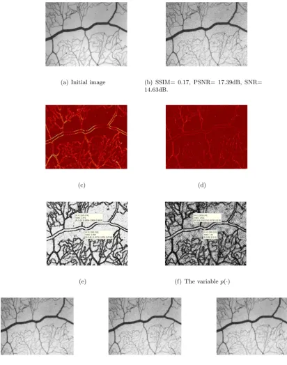
In Figure 1, we consider a medical image available from the internet which is corrupted by speckle noise with variance σ2 = 0.04. The images illustrated below show the original image, noisy one, the topological gradient indicator for the second- and fourth-order PDE, and the variables exponent functions p(_·) andq(_·). Here, we test the efficiency and the performance of the proposed approach for important feature detection of blood vessels and veins. The images 1(c) and 1(d) show the topological gradient indicator for the second- and fourth-order operator, respectively. We can see that the topolog-ical gradient of the fourth-order PDE able to see more information about the objects presented here. However, the topological gradient indicator for the second-order PDE is carried for the detection of edges doesn’t perform to detect objects of smaller pixels. The images 1(e) and 1(f) show the variables exponent q(·) and p(·), respectively. The visualization of the variable exponents are depend on the topological gradient, however, for the important feature having the value of q(·) andp(·) near to 1 to slow down diffusion, we can also see from images 1(e) and 1(f) the values of the variable exponents ranging from 1 to 2 and the object detected by the second-order derivative are very thin.

We note that from Figure 1 the restoration result obtained by thep(_·)-Kirchhoff model (see image 1(g)) gives better result than the TVL model (see image 1(h)) and the Bi-Harmonic model (see image 1(i)). We can deduce that the three models give good results with minor differences which are compared quantitatively by using the PSNR, SNR and SSIM indicators. We can also learn from the p(_·)-Kirchhoff model that the variable exponents p(_·) and q(_·) can be considered as a sort of segmentation and important features detection.

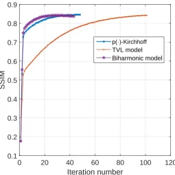
Figure 2 shows the convergence of the split Bregman scheme for the three models. We compared between those models by using the number of iterations as function of the SSIM indicator. We can see that the SSIM indicator for the p(_·)-Kirchhoff model speedely tends to 0.84 after 48 iterations. However, the SSIM indicator of the TVL model converges monotonically and slowly to 0.84 after 101 iterations. This isn’t surprising result since the ∆_|∆_∆·_·| and div_|∇·|∇· have slow impact on smoothness. The SSIM of the “Bi-Harmonic model” tends to 0.83 after only 39 iterations, it is due to the high frequency of the biLaplace, ∆2_{·, operator. From these images we can conclude that the} “Bi-Harmonic model” is not stable with respect to the number of iterations, however at the iteration 42 it diverges (see Figure 2). The p(·)-Kirchhoff and TVL models give the same value of SSIM, their main deference is the number of iterations.

3(e) the objects detected and do not have jump across the discontinuity.

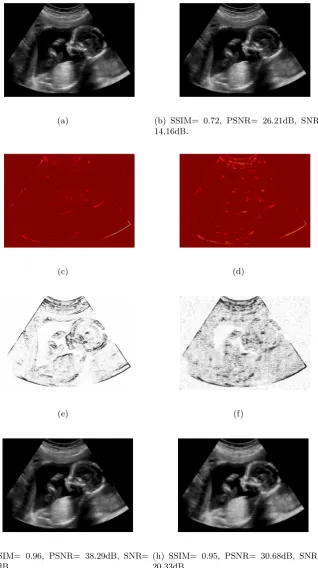
We can show the performance of our model for a more specific ultrasound medical images. From Figure 4, we can see that thep(·)-Kirchhoff model gives a good result compared with the TVL model, however the result in 4(g) is very semilar to the original one. From the figure 4(h), we can see that the TVL admits a strong smoothing rate on the medical images and one can also see white contrasts on some regions. When we zoom we can see in Figure 5 a comparison between thep(_·)-Kirchhoff model, and the TVL model. For the TVL model we can see that the image is very smooth and we show artifacts (some white points) near the edges of the image and this due to the singularity of the total variation.

7

Conclusion

In this paper, we have presented a new approach to restore images corrupted by speckle multiplica-tive noise. The proposed approach combines the advantages of the topological gradient method for important feature detection and the anisotropic diffusion model based on thep(_·)-Kirchhoff operator for the denoising. In the numerical computation, we used the split Bregman method in order to solve the nonlinear equation. The experiment results show the good quality in the recovering of the edges and thin structures as well as the image denoising.

References

[1] Mostafa Allaoui. Existence of three solutions for variable exponent elliptic systems. ANNALI DELL’UNIVERSITA’DI FERRARA, 61(2):241–253, 2015.

[2] Samuel Amstutz and J´erˆome Fehrenbach. Edge detection using topological gradients: A scale-space approach. J. Math. Imaging Vis., 52(2):249–266, 2015.

[3] Samuel Amstutz, Imen Horchani, and Mohamed Masmoudi. Crack detection by the topological gradient method. Control and Cybernetics, 34(1):81–101, 2005.

[4] Samuel Amstutz, Antonio Andre Novotny, and Nicolas Van Goethem. Topological sensitivity analysis for high order elliptic operators. preprint, 2012.

[5] Samuel Amstutz, Antonio Andre Novotny, and Nicolas Van Goethem. Topological sensitivity anal-ysis for elliptic differential operators of order 2m. Journal of Differential Equations, 256(4):1735– 1770, 2014.

[6] Gilles Aubert and Audric Drogoul. Topological gradient for a fourth order operator used in image analysis. ESAIM: Control, Optimisation and Calculus of Variations, 21(4):1120–1149, 2015.

[7] Didier Auroux. From restoration by topological gradient to medical image segmentation via an asymptotic expansion. Math. Comput. Model., 49(11):2191–2205, 2009.

[8] Marino Belloni and Bernd Kawohl. A direct uniqueness proof for equations involving the p-Laplace operator. Manuscripta Mathematica, 109(2):229–231, 2002.

[9] Martin Benning, Christoph Brune, Martin Burger, and Jahn M¨uller. Higher-order TV methods enhancement via Bregman iteration. Journal of Scientific Computing, 54(2-3):269–310, 2013.

[11] Jean Cea. Conception optimale ou identification de formes, calcul rapide de la d´eriv´ee direction-nelle de la fonction coˆut.ESAIM: Mathematical Modelling and Numerical Analysis, 20(3):371–402, 1986.

[12] Jean C´ea, St´ephane Garreau, Philippe Guillaume, and Mohamed Masmoudi. The shape and topological optimizations connection. Comput. Methods Appl. Mech. Engrg., 188(4):713–726, 2000.

[13] Tony Chan, Antonio Marquina, and Pep Mulet. High-order total variation-based image restora-tion. SIAM Journal on Scientific Computing, 22(2):503–516, 2000.

[14] Yunmei Chen, Stacey Levine, and Murali Rao. Variable exponent, linear growth functionals in image restoration. SIAM Journal on Applied Mathematics, 66(4):1383–1406, 2006.

[15] Lars Diening, Petteri Harjulehto, Peter H¨ast¨o, and Michael Ruzicka. Lebesgue and Sobolev spaces with variable exponents. Springer, 2011.

[16] Audric Drogoul. Numerical analysis of the topological gradient method for fourth order models and applications to the detection of fine structures in imaging.SIAM Journal on Imaging Sciences, 7(4):2700–2731, 2016.

[17] David Edmunds and Jiˇr´ı R´akosn´ık. Sobolev embeddings with variable exponent. Studia Mathe-matica, 143(3):267–293, 2000.

[18] David E Edmunds and Jiˇr´ı R´akosn´ık. Sobolev embeddings with variable exponent, ii. Mathema-tische Nachrichten, 246(1):53–67, 2002.

[19] Abdelrachid El Amrouss, Fouzia Moradi, and Mimoun Moussaoui. Existence of solutions for fourth-order PDEs with variable exponents. Electronic Journal of Differential Equations, 2009(153):1–13, 2009.

[20] Xianling Fan, Jishen Shen, and Dun Zhao. Sobolev embedding theorems for spaces Wk,p(x). Journal of Mathematical Analysis and Applications, 262(2):749–760, 2001.

[21] Xianling Fan and Dun Zhao. On the spacesLp(x)_andWm,p(x)_{. Journal of Mathematical Analysis} and Applications, 263(2):424–446, 2001.

[22] Roberta Filippucci, Patrizia Pucci, and Fr´ed´eric Robert. On a p-Laplace equation with multiple critical nonlinearities. Journal de Math´ematiques Pures et Appliqu´ees, 91(2):156–177, 2009.

[23] St´ephane Garreau, Philippe Guillaume, and Mohamed Masmoudi. The topological asymptotic for PDE systems: The elasticity case. SIAM J. Control Optim., 39(6):1756–1778, 2000.

[24] Pascal Getreuer. Rudin-Osher-Fatemi Total Variation denoising using Split Bregman. Image Processing On Line, 2:74–95, 2012.

[25] Pascal Getreuer. Total Variation deconvolution using split Bregman. Image Processing On Line, 2:158–174, 2012.

[26] Pascal Getreuer. Total Variation inpainting using split Bregman. Image Processing On Line, 2:147–157, 2012.

[28] P. Harjulehto, P. H¨ast¨o, V. Latvala, and O. Toivanen. Critical variable exponent functionals in image restoration. Applied Mathematics Letters, 26(1):56 – 60, 2013.

[29] Lamia Jaafar Belaid, Mohamed Jaoua, Mohamed Masmoudi, and Lassaad Siala. Application of the topological gradient to image restoration and edge detection. Engineering Analysis with Boundary Elements Journal, 32(11):891–899, 2008.

[30] Zhengmeng Jin and Xiaoping Yang. A variational model to remove the multiplicative noise in ultrasound images. J. Math. Imaging Vis., 39(1):62–74, 2011.

[31] Karl Krissian, Ron Kikinis, Carl Fredrik Westin, and Kirby Vosburgh. Speckle-constrained filter-ing of ultrasound images. In 2005 IEEE Computer Society Conference on Computer Vision and Pattern Recognition (CVPR’05), volume 2, pages 547–552, 2005.

[32] Fang Li, Zhibin Li, and Ling Pi. Variable exponent functionals in image restoration. Applied Mathematics and Computation, 216(3):870 – 882, 2010.

[33] Peter Lindqvist. Notes on thep-Laplace Equation. University of Jyv¨askyl¨a - Lectures notes, 2006.

[34] Thanasis Loupas. Digital image processing for noise reduction in medical ultrasonics. PhD thesis, University of Edinburgh, UK, 1988.

[35] Mohamed Masmoudi. The topological asymptotic. In R. Glowinski, H. Kawarada, and J. Periaux, editors, Computational Methods for Control Applications, volume 16 of Math. Sci. Appl., pages 53–72. GAKUTO International, 2002.

[36] Konstantinos Papafitsoros, Carola Bibiane Schoenlieb, and Bati Sengul. Combined First and Second Order Total Variation Inpainting using Split Bregman. Image Processing On Line, 3:112– 136, 2013.

[37] Konstantinos Papafitsoros and Carola-Bibiane Sch¨onlieb. A combined first and second order variational approach for image reconstruction. Journal of Mathematical Imaging and Vision, 48(2):308–338, 2014.

[38] Michael Ruzicka. Electrorheological fluids: modeling and mathematical theory. Springer Science & Business Media, 2000.

[39] Jan Sokolowski and Antoni Zochowski. On the topological derivative in shape optimization.SIAM J. Control Optim., 37(4):1251–1272, 1999.

[40] Carsten Steger. Extracting curvilinear structures: A differential geometric approach. InEuropean Conference on Computer Vision, pages 630–641. Springer, 1996.

[41] Carsten Steger. An unbiased detector of curvilinear structures. IEEE Transactions on Pattern Analysis and Machine Intelligence, 20(2):113–125, 1998.

[42] Yilun Wang, Junfeng Yang, Wotao Yin, and Yin Zhang. A new alternating minimization algo-rithm for total variation image reconstruction. SIAM Journal on Imaging Sciences, 1(3):248–272, 2008.

[44] Y. L. You and M. Kaveh. Fourth-order partial differential equations for noise removal. IEEE Transactions on Image Processing, 9(10):1723–1730, 2000.

(a) Initial image (b) SSIM= 0.17, PSNR= 17.39dB, SNR= 14.63dB.

(c) (d)

[X,Y]: [305 312] Index: 1.058 [R,G,B]: [0.2078 0.2353 0.6745] [X,Y]: [225 174]

Index: 1.971 [R,G,B]: [0.9804 0.9804 0.9804]

(e)

[X,Y]: [305 312] Index: 1.01 [R,G,B]: [0 0 0] [X,Y]: [225 174] Index: 1.921 [R,G,B]: [0.9176 0.9176 0.9176]

(f) The variablep(·)

(g) SSIM= 0.847, PSNR= 29.3dB, SNR= 26.52dB, 48 iterations.

(h) SSIM= 0.842, PSNR= 28.58dB, SNR= 25.97dB, 101 iterations.

(i) SSIM= 0.837, PSNR= 27.79dB, SNR= 25.19dB, 39 iterations.

Iteration number

0 20 40 60 80 100 120

SSIM

0.1 0.2 0.3 0.4 0.5 0.6 0.7 0.8 0.9

p(_·)-Kirchhoff TVL model Biharmonic model

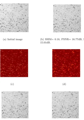
(a) Initial image (b) SSIM= 0.18, PSNR= 16.77dB, SNR= 15.01dB.

(c) (d)

(e) SSIM= 0.7, PSNR= 25.74dB, SNR= 24.03dB, 41 iterations.

(f) SSIM= 0.66, PSNR= 23.44dB, SNR= 21.83dB, 57 iterations.

(g) SSIM= 0.67, PSNR= 24.41dB, SNR= 22.8dB, 32 iterations.

(a) (b) SSIM= 0.72, PSNR= 26.21dB, SNR= 14.16dB.

(c) (d)

(e) (f)

(g) SSIM= 0.96, PSNR= 38.29dB, SNR= 26.08dB.

(h) SSIM= 0.95, PSNR= 30.68dB, SNR= 20.33dB.

(a) Initial image (b) SSIM= 0.55, PSNR= 21dB, SNR= 12.77dB.

(c) (d)

(e) (f)

(g) SSIM= 0.868, PSNR= 30dB, SNR= 21.62dB, 44 iterations.

(h) SSIM= 0.861, PSNR= 29.36dB, SNR= 20.98dB, 51 iterations.

(i) SSIM= 0.867, PSNR= 29.91dB, SNR= 21.53dB, 46 iterations.