Vol. 11 (2017) 4323–4346 ISSN: 1935-7524
DOI:10.1214/17-EJS1318
Nonparametric estimating equations for
circular probability density functions
and their derivatives
Marco Di Marzio and Stefania Fensore
DMQTE,
Universit`a di Chieti-Pescara, Viale Pindaro 42, 65127 Pescara, Italy
e-mail:[email protected];[email protected]
Agnese Panzera
DiSIA, Universit`a di Firenze,
Viale Morgagni 59, 50134 Firenze, Italy e-mail:[email protected]
and
Charles C. Taylor
Departement of Statistics, University of Leeds, Leeds LS2 9JT, UK e-mail:[email protected]
Abstract: We propose estimating equations whose unknown parameters are the values taken by a circular density and its derivatives at a point. Specifically, we solve equations which relate local versions of population trigonometric moments with their sample counterparts. Major advantages of our approach are: higher order bias without asymptotic variance inflation, closed form for the estimators, and absence of numerical tasks. We also investigate situations where the observed data are dependent. Theoretical results along with simulation experiments are provided.
Keywords and phrases: Circular kernels, density estimation, Fourier coefficients, jackknife, sin-polynomials, trigonometric moments, von Mises density.
Received July 2016.
1. Introduction
Circular data occur when the sample space is described by a circle, as opposed to the real line in standard statistics. They often arise in biology (migration paths of animals), meteorology (wind and marine current directions), and geology (orientations of joints and faults, landforms, oriented stones). Other examples include phenomena that are periodic in time, like daily and seasonal
economic phenomena. If compared to a linear scale, a circular one has special features. Firstly, the beginning and the end of the measurement scale coincide, and their common location is called the origin (or zero direction). This latter is arbitrary, and likewise any designation of median, high or low values. Also note that for circular data there is no concept of standardisation. The only data transformations which do not change the relative positions of the observations are rotation and reflection.
Nonparametric circular density estimation could be seen as a non-mature research field. Although basic kernel density estimation is well known (see, for example, [6], [2], [8] and [14]), not much has been written on more sophisti-cated methods, aimed at bias reduction. This would be useful for efficient point estimation in the cases of heavy density tails, multi-modality or asymmetry. Additionally, it would improve the precision in estimating a confidence interval for the value of the density at a point, or confidence bands for the whole density. Indeed, it is well known that the bias of nonparametric methods leads to in-correct centring of the confidence interval with severe consequences on coverage probability. In the Euclidean setting small bias methods have been suggested as a remedy, for example, by [1] and [5].
In this paper we propose estimating equations for circular density estimation (and its derivatives) where local versions of population trigonometric moments are equated with their empirical counterparts. We model the unknown density by a periodic series expansion whose coefficients are the system variables. There-fore, we estimate the value of functions at a point, as opposed to the classical method of moments which is used for global parameters. It will be seen that modelling via longer series will give smaller asymptotic bias without asymptotic variance inflation. The system is linear and has a closed-form solution, so our estimators have a general formulation depending on both expansion degree and the order of the target derivative.
In Section2we obtain the estimators. Some interpretative reasoning connect them to previous Euclidean literature based on quite different ideas. In Section 3 we first derive general asymptotic properties, then we focus on von Mises kernel theory. Finally, in Section 4 we show how the method performs, using simulation experiments and real data case studies, also through a comparison with other methods existing in the literature.
2. The estimators
Thethtrigonometric moment (about the zero direction)of the absolutely con-tinuous distribution function F of a circular random variable Θ is defined as
a+ ib, ∈N, where i2=−1, anda andb stand for theth cosine and sine
moments respectively, i.e.
a:=E[cos(Θ)] = π
−π
cos(α)dF(α), b:=E[sin(Θ)] = π
−π
sin(α)dF(α).
Any distribution on the circle is determined by its characteristic function, and this uniqueness property, differently from the Euclidean setting, assures that they are determined by their moments. Assuming that F admits continuous derivatives up to orderp+ 1 atθ∈[−π, π),p∈N, thenf(α) :=F(1)(α) can be approximated by the sin-polynomial
˜
fp(α;θ) := p
j=0
f(j)(θ) sinj(α−θ)
j!
with negligible error if |α−θ| is small. We can interpret ˜fp(α;θ) as a
(trun-cated) Taylor-like expansion suited for functions defined on a circle because its increment has periodic nature. In fact, the sine function preserves the sign of α−θ, and also takes small values whenαandθ are separated by a very small arc. Notice that, if the arc contains the origin, this latter property does not hold for the simple difference.
Nonparametric estimating equations could be obtained by matching sample moments to their correspondingapproximated theoretical ones given by
π
−π
cos(α) ˜fp(α;θ)dα,
π
−π
sin(α) ˜fp(α;θ)dα,
with density derivatives at θ ∈ [−π, π), from order 0 up to order p, which constitute the system variables. However, recalling thatf(α) issatisfyingly ap-proximated by ˜fp(α;θ) only ifαbelongs to a narrow neighbourhood of θ, and
Definition 2.1. Let Kκ denote a generic circular kernel with concentration
parameter κ∈ (0,∞) (see [2]). For ∈N, we define the th local trigonomet-ric (resp. cosine and sine) moments, at θ ∈ [−π, π), of a circular distribution functionF the quantities
a(θ) := π
−π
Kκ(α−θ) cos(α)f(α)dα, b(θ) := π
−π
Kκ(α−θ) sin(α)f(α)dα.
The idea is that above local moments are essentially determined by the values taken by integrands over a tight interval centred at θ, where approximation
˜
fp is reliable. Tightness inversely depends on the magnitude of concentration
parameter κ. As a simple parallel with Euclidean kernel density estimation, we would say that κ moves toward the same direction as the inverse of the bandwidth.
Then, our simultaneous equations would be based on quantities reported in
Definition 2.2. Let Kκ denote a generic circular kernel with concentration
parameterκ∈(0,∞). We defineapproximated local trigonometric (resp. cosine and sine) moments of order∈Natθ∈[−π, π) of a circular distribution with densityf the quantities
p
j=0
f(j)(θ)cj(θ) and
p
j=0
f(j)(θ)sj(θ), (2.1)
where
cj(θ) :=
π
−π
Kκ(α−θ) cos(α)
1 j!sin
j(α−θ)dα,
and
sj(θ) :=
π
−π
Kκ(α−θ) sin(α)
1 j!sin
j(α−θ)dα.
Letting Θ1, . . . ,Θn be a random sample of angles from the unknown density f,
sample local trigonometric (resp. cosine and sine) moments atθare defined as
C(θ) := n
i=1Kκ(Θi−θ) cos(Θi)
n and S(θ) :=
n
i=1Kκ(Θi−θ) sin(Θi)
n .
Notice that, for fixednandθ, a trade-off in selecting the value of parameterκ arises. In fact, on the population side of above definition, we have observed that a big κ ensures accuracy of expansion. On the other hand, sample quantities require maximize the amount of data effectively participating to the estimation process, and this is produced through a small κ. This suggests to formulateκ as an increasing function ofn.
Regarding asymptotic accuracy, other than the obvious convergence of the sums to integrals, we would require that quantities in Equation (2.1) satisfyingly approximate a(θ) and b(θ), respectively. This is easily seen to be the case if
properties, obviously the use of sin-polynomials along with circular kernels will guarantee estimators that are both periodic and rotationally invariant.
Importantly, the facts that most of circular kernels can be approximated by Euclidean ones if their concentration parameter is big, and that in a neighbour-hood of 0 we have sin(x) ≈ xcould misleadingly suggest that, under certain asymptotic conditions, they could be successfully employable also when data have periodic nature. But this does not hold because linear kernels are guaran-teed to give estimates that are a)severely wrong in a region around the origin (potentially the whole circle); b) not rotationally invariant. This has a strong practical relevance when considering that the choice of origin is arbitrary.
From now on, we assume Kκ to be a second sin-order circular kernel with
concentration parameterκ∈(0,∞) (see [2]), i.e. a 2π-periodic density function admitting the absolutely convergent Fourier series representation
Kκ(α) =
1 + 2∞j=1γj(κ) cos(jα)
2π .
Remark 2.1. The particular case of no concentration gives constant weights, formally asκ→0,Kκ(α)→(2π)−1. This makes the estimate independent on
the data. For example, setting both κand pto zeroalways yields an uniform density (see also Section2.1). Curiously, for real-line kernel methods the shape of the estimate is never perfectly independent on the specific sample at hand. In fact, a positive weight fixed over the whole support still gives estimates that are not constant for finite samples due to the unavoidable presence of boundaries.
Note that γ0(κ) = 1. Moreover, the second sin-order implies thatc0 0(θ) = 1 and c20(θ) = 0, while due to the symmetry of Kκ, cj0(θ) = 0 for odd j. For ≥0 andj ≥0, direct calculation, involving Fourier coefficients, gives general expressions as follows
cj(θ) =
⎧ ⎪ ⎨ ⎪ ⎩ 1
j!2j
j s=0
j s
(−1)s+(j+1)/2γ
|−j+2s|(κ) sin(θ) ifj is odd,
1
j!2j
j s=0
j s
(−1)s+j/2γ
|−j+2s|(κ) cos(θ) ifj is even, (2.2)
and
sj(θ) =
⎧ ⎪ ⎨ ⎪ ⎩ 1
j!2j
j s=0
j s
(−1)s+1+(j+1)/2γ|−j+2s|(κ) cos(θ) ifj is odd,
1
j!2j
j s=0
j s
(−1)s+j/2γ
|−j+2s|(κ) sin(θ) ifj is even.
(2.3) For apth order approximation the estimating equations havep+1 unknowns. With the aim of including complete trigonometric moments in the system, we need to start from order zero (which produces a single equation becausesj0(θ) =
2.1. Even p
When the sin-polynomial degreepis even, simultaneous equations are obtained by including local trigonometric moments from order 0 up to order p/2. In matrix form these can be expressed as
Bpβ =M, (2.4)
where
β := (β0β1 . . . βp),
M := (C0(θ)C1(θ)S1(θ) . . . C
q(θ)Sq(θ)),
and
Bp :=
⎛ ⎜ ⎜ ⎜ ⎜ ⎜ ⎜ ⎜ ⎝
1 c1
0(θ) . . . c
p
0(θ) c0
1(θ) c11(θ) . . . c
p
1(θ) s0
1(θ) s11(θ) . . . s
p
1(θ) ..
. ... . .. ... c0
q(θ) c1q(θ) . . . cpq(θ)
s0
q(θ) s1q(θ) . . . spq(θ) ⎞ ⎟ ⎟ ⎟ ⎟ ⎟ ⎟ ⎟ ⎠
.
The density estimator is defined to be the solution forβ0, i.e.
ˆ
f(θ;p) :=|Ap|
|Bp|, (2.5)
whereApis the same asBpbut with the first column replaced byM. Elementary
orthogonality arguments prove that bothAp andBp have full rank.
Remark 2.2. Note that using expressions (2.2) and (2.3) in the general solution (2.5) leads to explicit closed-form solutions for the estimators whatever the kernel is. In particular, Cramer’s rule is not used as a numerical algorithm, since it is known to be expensive and unstable, but only as a way to represent exact solutions of the system, which will are seen to be convenient for various asymptotic considerations.
Clearly, recalling that Kκ = 1, we see that the case p = 0 yields the
standard kernel density estimator
ˆ
f(θ; 0) = 1 n
n
i=1
Kκ(Θi−θ).
When Kκ is a von Mises kernel, i.e. γj(κ) = Ij(κ)/I0(κ), with Ij, j ∈ N,
denoting the modified Bessel function of first kind and order j, the estimator forp= 2 has the following simple form
ˆ
f(θ; 2) =I0(κ)I2(κ) ˆf(θ; 0)− I 2
1(κ) ˆf(θ; 1)
I0(κ)I2(κ)− I2 1(κ)
that is a linear combination of density estimators with p= 0 andp= 1 (for a definition of the latter see formula (2.8) in the next section). Such a structure (which will generally result in an estimator which is not non-negative forp= 0) is reminiscent of thejackknifetechnique, as originally formulated by [10], where a density estimator is defined as a linear combination of two distinct ones in order to get bias reduction.
The solution for βj, j ∈ (1, . . . , p), of the above system gives estimator for
f(j)(θ), which is
ˆ
f(j)(θ;p) :=|A
j p|
|Bp|
,
whereAj
pis the same ofBp, but with the (j+1)th column replaced byM. Notice
that in the first equation of system (2.4), recalling that for odd j cj0 = 0, the coefficientsβjdisappear. This in turn implies the same odd derivative estimators
as for thep−1 degree.
2.2. Odd p
When the sin-polynomial degree p is odd, we consider the matching between local trigonometric moments from order 1 up to order (p+ 1)/2, obtaining the following system expressed in matrix form
Dpβ=N,
where Dp andN are defined asBp andMwith, respectively, the first row and first element omitted. The solution forβ0gives the estimator
ˆ
f(θ;p) := |Cp|
|Dp|, (2.7)
whereCphas the same columns ofDp, except the first one which is replaced by
N. The same arguments as in the previous section prove that bothCp andDp
have full rank, also Remark (2.2) applies.
The use of a von Mises kernel yields simple estimators forp= 1 and p= 3, as follows
ˆ
f(θ; 1) = 1 2πnI1(κ)
n
i=1
cos(Θi−θ) exp(κcos(Θi−θ)), (2.8)
ˆ
f(θ; 3) = w(κ) ˆf(θ; 1) +κ 2I
2(κ)2πn1
n
i=1cos(2Θi−2θ) exp(κcos(Θi−θ))
w(κ) +κ2I2(κ)2 ,
(thinner). The cubic fit is reminiscent of the jackkinife technique observed in expression (2.6). Concerning derivative estimators, the solution of the above system forβj,j∈(1, . . . , p), yields
ˆ
f(j)(θ;p) := |C
j p|
|Dp|,
withCj
pbeing the same asDp, but with the (j+ 1)th column replaced by N.
3. Large samples results
A fundamental assumption made in this section is that the concentration pa-rameter of the kernelκ=κn is an increasing function of sample sizen. To keep
notation less cumbersome, such dependence will be suppressed. The bias of ˆf(θ;p) is obtained in the following
Result 3.1. Given the random sample of anglesΘ1, . . . ,Θn from the unknown
densityf, consider estimators (2.7) and (2.5) for odd and even p, respectively. Assume that
i) Kκ is a second sin-order circular kernel whose Fourier coefficients strictly
increase withκ; ii) limn→∞κ=∞;
iii) f is(p+1)-times and(p+2)differentiable for odd and evenp, respectively. Then, for oddp
E[ ˆf(θ;p)]−f(θ) = |C˜p|
|Dp|f
(p+1)(θ) +o
|C˜
p|
|Dp|
,
whereCp˜ is the same asCp, but with the first column replaced by
cp1+1(θ) sp1+1(θ) . . . c(pp+1+1)/2(θ) sp(p+1+1)/2(θ)
,
while, for evenp,
E[ ˆf(θ;p)]−f(θ) =|Ap˜ |
|Bp|f
(p+2)(θ) +o
|Ap˜ |
|Bp|
,
withAp˜ being the same asAp, but with the first column replaced by
cp0+2(θ) cp1+2(θ) sp1+2(θ) . . . cpp/+22(θ) spp/+22(θ)
.
Circularity makes the normalization of the estimates easily tractable. Indeed, we have just seen thatE[ ˆf(θ;p)] is asymptotically formulated as a sum between f(θ) and a linear combination of the derivatives of f atθ. Now, from the fact that derivatives of a circular density function are obviously periodic functions, it follows from Fubini’s theorem that the expectation of the area of the estimate is equal to one, without regard to the values of p and κ. This comes in stark contrast with Euclidean higher order bias theory.
Concerning the variance, we get the following
Result 3.2. Given the random sample of anglesΘ1, . . . ,Θn from the unknown
densityf, consider estimator (2.7) for oddp((2.5) for evenp, respectively). Let Mij denote the(i, j)minor ofCp (Ap, resp.). Then, we have
Var[ ˆf(θ;p)] = 1 V2
p ⎧ ⎨ ⎩
p+1
i=1
Mi21Var[ai1] + 2
i=j
(−1)(i+j)Mi1Mj1Cov[ai1, aj1] ⎫ ⎬ ⎭,
(3.1) where aij stands for the (i, j)th entry of Cp (Ap, resp.), Vp :=|Dp| (Vp:=|Bp|,
resp.). Specifically, the possible covariance expressions, under assumptions of Result 3.1, for (, m)∈N×Nand≥m, omittingO(n−1)terms, are
Cov[C(θ),Cm(θ)] =
f(θ)
4nπ {cos((−m)θ)P(, m) + cos((+m)θ)Q(, m)}, Cov[S(θ),Sm(θ)] =
f(θ)
4nπ {cos((−m)θ)P(, m)−cos((+m)θ)Q(, m)}, Cov[S(θ),Cm(θ)] =
f(θ)
4nπ {sin((m−)θ)P(, m) + sin((+m)θ)Q(, m)}, Cov[Sm(θ),C(θ)] =
f(θ)
4nπ {sin((−m)θ)P(, m) + sin((+m)θ)Q(, m)}, with
P(, m) :=
−m
i=0
γi(κ)γ−m−i(κ) + 2
∞
i=−m+1
γi(κ)γi−(−m)(κ),
Q(, m) :=
+m−1
i=1
γi(κ)γ+m−i(κ) + 2
∞
i=0
γi(κ)γ+m+i(κ).
Proof. See Appendix.
Asymptotic normality of ˆf(θ;p), for both even and odd p, can be easily demonstrated starting from the fact that both |Ap| and |Bp|are linear combi-nations of sample averages of independent and identically distributed random variables.
3.1. Von Mises kernel theory
with respect to the kernel, and therefore Fourier coefficients remain unspecified. However, it is well known that in local density estimation the choice of the kernel is generally not considered an important task. Specifically, we could select whatever kernel showing uni-modality, symmetry, smoothness,rapidlydecaying tails to zero and that is able to concentrate its whole mass around zero. Now, well known circular densities that are uni-modal and symmetric are: triangular, cardioid, wrapped Cauchy, von Mises and wrapped normal.
Once said that the first one is not smooth enough, the second one is not able to indefinitely concentrate, and that the third one has too heavy tails, von Mises and wrapped normal densities remain to us. However, since from moderate concentration and upwards they have nearly identical shape, their use gives generally same results. These considerations suggest that restricting the theory to von Mises kernel is not a severe choice.
In what follows we show how using the von Mises density as the kernel leads to a number of interesting considerations. The asymptotic bias of ˆf(θ;p) for some values ofpis obtained in the following
Result 3.3. Given a random sample of angles Θ1, . . . ,Θn, from the unknown
density f, consider estimator fˆ(θ;p), θ∈ [−π, π), with Kκ being a von Mises
kernel. Assuming thatκ→ ∞ asn→ ∞,
E[ ˆf(θ; 0)]−f(θ) = 1 κ
I1(κ) 2I0(κ)f
(2)(θ) +o
1 κ
E[ ˆf(θ; 1)]−f(θ) = 1 κ
I2(κ) 2I1(κ)f
(2) (θ) +o
1 κ
,
and
E[ ˆf(θ; 2)]−f(θ) = 1 κ2
{I2
2(κ)− I1(κ)I3(κ)} 8{I0(κ)I2(κ)− I2
1(κ)}
f(4)(θ) +o
1 κ2
.
Proof. See Appendix.
Comparing the asymptotic bias of the local constant and the local linear fit, we see that, despite both have the same magnitude, the local linear one is smaller than the constant one for each value ofκ. This is in clear contrast with ordinary polynomial fitting, where the relative merits depend on the estimation point. Forp= 2, the asymptotic bias isO(1/κ2), and so the jackknife idea works by cancelling the larger bias term.
Concerning the variance, asymptotic results for some values ofpare collected in the following
Result 3.4. Given a random sample of angles Θ1, . . . ,Θn, from the unknown
density f, consider estimator fˆ(θ;p), θ ∈ [−π, π), equipped with a von Mises kernel. Assuming thatκ/n→0 asn→ ∞
Var[ ˆf(θ; 0)] = f(θ) n
I0(2κ) 2πI2
0(κ) +O
1 n
Var[ ˆf(θ; 1)] =f(θ) n
I0(2κ) +I2(2κ) 4πI2
1(κ)
+O
1 n
, (3.3)
and
Var[ ˆf(θ; 2)] = f(θ) n ×
I0(2κ)[I2
1(κ) + 2I22(κ)] +I1(κ)[I1(κ)I2(2κ)−4I2(κ)I1(2κ)] 4π{I2
1(κ)− I0(κ)I2(κ)}2
+O
1 n
.
Proof. See Appendix.
Using the properties of Bessel functions, we can see that, for big enoughκ, the asymptotic variances in the above result have magnitude O(√κ/n). However, when comparing p= 0 and p = 1, we observe a phenomenon similar to that seen for biases, but in this case the superiority is on the local constant side. Moreover, concerning asymptotic behaviour of the quadratic fit, we have
lim
κ→∞
V ar[ ˆf(θ; 2)] V ar[ ˆf(θ; 0)] =
27 16.
These results clearly indicate that fitting a quadratic polynomial would be convenient when the bias is severe: in fact, we observe a variance inflation, inevitably produced by the need of estimating more parameters, that with a big enough sample size will be dominated by bias reduction.
Concerning the smoothing degree, settingR(g) :=−ππg2(α)dα, for a square integrable functiong, we get
Result 3.5. Given a random sample of angles Θ1, . . . ,Θn from the unknown
density f, consider estimatorfˆ(θ;p),θ ∈[−π, π), having the von Mises kernel as the weight function. The value of κ which minimizes the asymptotic mean integrated squared error offˆ(·;p) withp∈(0,1)is
κAMISE=
2nπ1/2R
f(2)
2/5 ,
while, for p= 2,
κAMISE=
4 27nπ
1/2Rf(4) 2/9
.
Proof. See Appendix.
It follows that the rate of convergence of ˆf(θ;p) isn−4/5 for bothp= 0 and p= 1, while it isn−8/9 forp= 2. The rate of convergence for whatever orderp is provided by the following
Result 3.6. Given a random sample of angles Θ1, . . . ,Θn from the unknown
density f, consider estimator fˆ(θ;p), θ ∈[−π, π), with Kκ being a von Mises
Proof. See Appendix.
Finally, as circular samples often come in form of dependent data – think, for example, of direction of winds or marine currents taken at a given location within a period of time – it could be of interest to ensure the effect of some general dependence structures on our methods. In what follows we assume that data come from anα-mixing stochastic process.
Result 3.7. Let Θ1, . . . ,Θn be a realization of an α-mixing process. If
i) the mixing coefficients satisfy |α(ω)| ≤Q1ω−λ,ω ∈ Z, for positive con-stants Q1 andλ >2;
ii) the joint density g of (Θl,Θm) satisfies g∞ < ∞, for l ∈ (1, . . . , n), m∈(1, . . . , n);
then, for p∈N, the convergence rate of estimator f(θ;ˆ p),θ∈[−π, π), with the von Mises kernel is the same as the i.i.d. case.
Proof. See Appendix.
A similar result for kernel density estimator in the Euclidean multivariate setting can be found, for example, in [9].
4. Practical performance 4.1. Density estimation
This simulation study compares both best possible and practical performances of the estimators. As accuracy indicator we refer to integrated mean squared error (IMSE). Kernels used are von Mises probability density functions, denoted byvM(μ, κ), where parametersμandκindicate respectively the mean direction and the concentration parameter.
Whenp >0 our estimates are not guaranteed to bebona-fide. However, we have not correct them because elementary considerations say that the quantity
ˆ
f goes to one at the same rate as the asymptotic bias, and therefore the pointwise convergence rates of ˆf to f remain unaffected up to a coefficient equal to the value off atθ. As a final remark, we recall that the casep= 0 is the classical circular kernel density estimator, firstly proposed by [6]. Therefore, p = 0 is the best possible benchmark, useful to check practical utility of our proposals.
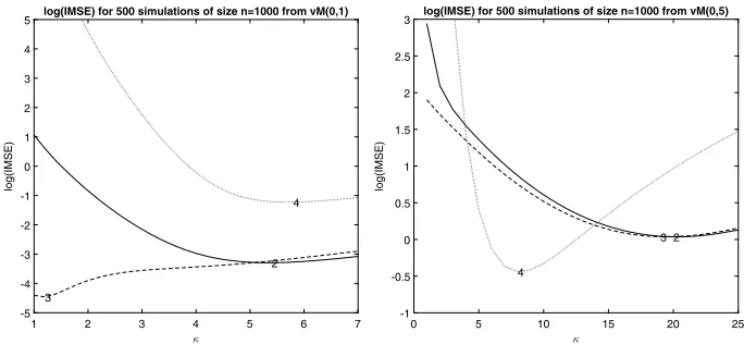
Fig 1. log(IMSE) for a range of values ofκforp= 0(solid),p= 1(dashed),p= 2(dotted), p= 3(dotdash) andp= 4(+) for 500 samples of sizen= 100(left) andn= 1000(right) from avM(0,1).
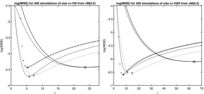
Fig 2. log(IMSE) for a range of values ofκforp= 0(solid),p= 1(dashed),p= 2(dotted), p= 3(dotdash) andp= 4(+) for 500 samples of sizen= 100(left) andn= 1000(right) from avM(0,5).
of these figures we use n = 1000. Since a bigger sample size leads to a more accurate estimate of the derivatives, we can see that the best performances are given by estimators of higher orders, because, in contrast with the casen= 100, bias reduction dominates variance inflation.
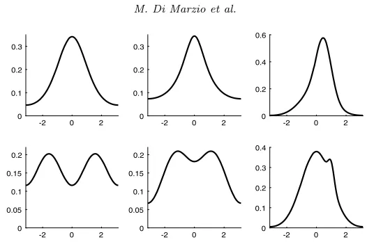
[image:13.612.108.450.112.268.2] [image:13.612.108.450.328.485.2]Fig 3. Population density models with parameters (mean direction, concentration) used for the simulation on density estimation. Top line, from left: von Mises(0,1); Wrapped Cauchy (0,1), equal mixture between two Wrapped Normals with parameters(0,1)and(0.5,0.5). Bot-tom line, from left: equal mixture between two Wrapped Normals with parameters(−π/2,1) and (π/2,1), equal mixture between two Wrapped Normals with parameters(−2π/5,1)and (2π/5,1), mixture between two Wrapped Normals with weights19/20and1/20, and parame-ters(0,1)and(1,0.2).
In a second experiment, we estimate various densities by selecting smooth-ing degree by simple least squares cross-validation. Our population models are represented in Figure 3. Other than the standard von Mises, we have consid-ered classical more difficult cases like multimodality, asymmetry or heavy tails. A promising estimator has been included as a competitor, other than stan-dard kernel density method (p= 0). It is the circular local likelihood method described in [3]. Such an estimator can be defined as a polynomial estimator derived starting from a likelihood score. The Authors present closed formulas for polynomial degrees 1 and 2. We have included here both of them. We use sample sizes equal to 100 or 500. They have been taken moderate in order to check usefulness of the methods in practical situations. Our theoretical results have already described the behaviour of our proposals for large samples.
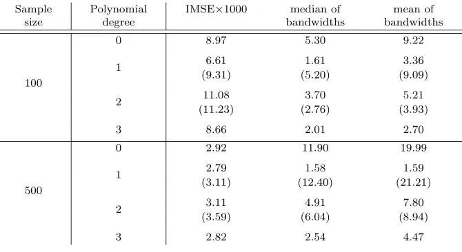
[image:14.612.200.463.91.265.2]Table 1
Comparison between proposed estimators and circular local likelihood ones (bracketed) in terms of average integrated squared errors (×1000) over 500 samples of sizes 100 or 500 drawn from avM(0,1)population. Median and mean of the smoothing degrees selected by
least-squares cross-validation.
Sample size
Polynomial degree
IMSE×1000 median of bandwidths
mean of bandwidths
100
0 7.32 4.10 7.55
1 5.51 1.66 3.27
(7.57) (3.97) (7.50)
2 9.49 3.34 4.25
(10.41) (3.14) (4.21)
3 7.09 1.77 2.23
500
0 2.05 8.10 11.45
1 1.60 1.60 2.02
(2.08) (8.07) (11.30)
2 2.06 4.13 5.19
(2.77) (5.52) (7.08)
3 1.61 2.30 2.69
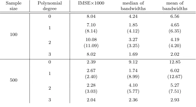
Table 2
Comparison between proposed estimators and (circular local likelihood ones) in terms of average integrated squared errors (×1000) over 500 samples of sizes 100 or 500 drawn from
awC(0,1)population. Median and mean of the smoothing degrees selected by least-squares cross-validation.
Sample size
Polynomial degree
IMSE×1000 median of bandwidths
mean of bandwidths
100
0 8.04 4.24 6.56
1 7.10 1.85 4.65
(8.14) (4.12) (6.35)
2 10.08 3.27 4.19
(11.09) (3.25) (4.20)
3 8.02 1.69 2.02
500
0 2.39 9.12 12.85
1 2.67 1.74 6.02
(2.40) (8.99) (12.67)
2 2.28 4.10 5.27
(3.03) (5.77) (7.51)
[image:15.612.112.447.463.646.2]Table 3
Comparison between proposed estimators and (circular local likelihood ones) in terms of average integrated squared errors (×1000) over 500 samples of sizes 100 or 500 drawn from
a0.5wN(0,1) + 0.5wN(.5, .5)population. Median and mean of the smoothing degrees selected by least-squares cross-validation.
Sample size
Polynomial degree
IMSE×1000 median of bandwidths
mean of bandwidths
100
0 12.52 10.90 17.13
1 14.35 8.89 13.67
(12.98) (10.54) (17.16)
2 11.44 4.06 5.89
(11.83) (2.78) (4.18)
3 11.08 2.56 3.68
500
0 3.57 21.96 32.76
1 4.30 20.57 29.77
(3.68) (22.52) (32.46)
2 2.86 5.97 8.23
(3.35) (6.43) (9.40)
3 3.14 4.38 5.64
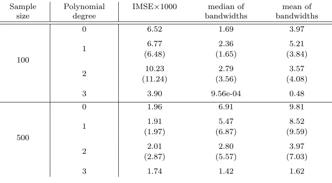
Table 4
Comparison between proposed estimators and (circular local likelihood ones) in terms of average integrated squared errors (×1000) over 500 samples of sizes 100 or 500 drawn from
a0.5wN(−π/2,1) + 0.5wN(π/2,1)population. Median and mean of the smoothing degrees selected by least-squares cross-validation.
Sample size
Polynomial degree
IMSE×1000 median of bandwidths
mean of bandwidths
100
0 6.52 1.69 3.97
1 6.77 2.36 5.21
(6.48) (1.65) (3.84)
2 10.23 2.79 3.57
(11.24) (3.56) (4.08)
3 3.90 9.56e-04 0.48
500
0 1.96 6.91 9.81
1 1.91 5.47 8.52
(1.97) (6.87) (9.59)
2 2.01 2.80 3.97
(2.87) (5.57) (7.03)
[image:16.612.166.500.462.646.2]Table 5
Comparison between proposed estimators and (circular local likelihood ones) in terms of average integrated squared errors (×1000) over 500 samples of sizes 100 or 500 drawn from
a0.5wN(−2π/5,1) + 0.5wN(2π/5,1)population. Median and mean of the smoothing degrees selected by least-squares cross-validation.
Sample size
Polynomial degree
IMSE×1000 median of bandwidths
mean of bandwidths
100
0 6.67 2.74 4.60
1 6.33 2.11 4.38
(6.89) (2.70) (5.32)
2 10.08 2.96 3.78
(10.96) (3.28) (3.93)
3 6.88 1.10 1.33
500
0 1.76 6.22 8.63
1 1.83 3.98 6.31
(1.80) (6.26) (8.57)
2 2.07 3.44 4.34
(2.80) (5.65) (6.78)
3 1.57 1.87 2.29
Table 6
Comparison between proposed estimators and (circular local likelihood ones) in terms of average integrated squared errors (×1000) over 500 samples of sizes 100 or 500 drawn from
a19/20wN(0,1) + 1/20wN(1,0.2)population. Median and mean of the smoothing degrees selected by least-squares cross-validation.
Sample size
Polynomial degree
IMSE×1000 median of bandwidths
mean of bandwidths
100
0 8.97 5.30 9.22
1 6.61 1.61 3.36
(9.31) (5.20) (9.09)
2 11.08 3.70 5.21
(11.23) (2.76) (3.93)
3 8.66 2.01 2.70
500
0 2.92 11.90 19.99
1 2.79 1.58 1.59
(3.11) (12.40) (21.21)
2 3.11 4.91 7.80
(3.59) (6.04) (8.94)
[image:17.612.111.446.462.645.2]4.2. Slope and curvature estimation
Using the same samples as the first case study, we have additionally estimated first and second derivatives. The results are reported in Figures4and5. We see that the interpretation given in Section4.1largely applies. Recalling that when pis even we have same odd derivative estimators as in thep−1 degree case, we show in Figure4only two curves.
Fig 4. log(IMSE) for a range of values of κ forp = 1and p = 2 (solid),p = 3and p = 4 (dashed) for 500 samples of size n = 1000 from a vM(0,1) (left) and vM(0,5) (right) comparing the first derivative estimation.
[image:18.612.162.503.219.375.2] [image:18.612.161.503.447.605.2]4.3. Application
To illustrate the methods on some real data we consider the arrival times of delayed planes in 2008. The full dataset is available from [7], but here we focus on two airlines (American AirlinesandContinental) and one airport (Atlanta). The arrival times are converted to the 24-hour clock (which is periodic) and all days of the year are included in the analysis. Overall, there were 2676 (AA) and 1278 (CO) delayed flights. A brief examination of the data shows that arrival times are recorded to an integer number of minutes, and there is a tendency to round to the nearest 5 minutes.
We considered density estimation with polynomial degrees p = 0,1 and 2, with smoothing parameters chosen by least squares cross-validation. The many coincident values in the data led to cross-validation selection ofκwhich diverged, so we “jittered” both datasets by adding random von Mises quantities with concentration 15.
Fig 6. Density estimation of arrival times of delayed flights for American Airlines (black) and Continental Airlines (red) using sin-polynomial degree p = 0(continuous) and p = 1 (dashed). The smoothing parameters were chosen by least-squares cross-validation.
[image:19.612.197.366.316.469.2]5. Discussion
In this paper we propose closed form estimators derived as a solution of a sys-tem of estimating equations. Other than having nice theoretical properties, our estimators seem to work satisfyingly in practical situations. As the consequence, methods for non-parametrically estimating a circular density, more sophisticated than traditional estimator presented in [6], seem a promising research field to pursue. We also introduce in circular statistics both simple formulas for local estimation of density derivatives and theory for the case of dependent observa-tions.
Our method makes possible to efficiently employa priori information on the smoothness of a circular density, especially when the curvature of the target population is pronounced. Surely, such a higher order differentiability can re-veal a disadvantage for making local moments less generally applicable than traditional circular kernel method.
A promising development for our approach could lie in replacing our series expansion by a circular parametric family. Here we would estimate optimal smoothing along with the density parameters. This would amount to a totally parametric method in correspondence of a null concentration of the kernel, as opposite to the situation described in Remark2.1.
Appendix
Proof of Result3.1. For odd (even, respectively)p, the result follows by observ-ing that the approximation ofE[C(θ)] and E[S(θ)], for ∈(1, . . . ,(p+ 1)/2)
( ∈ (0, . . . , p/2), resp.), by expansion (2) for f around θ up to order (p+ 1) ((p+ 2), resp), yields
E[C(θ)] = rp
j=0
cj(θ)f(j)(θ) +o crp
(θ)
,
and
E[S(θ)] = rp
j=0
sj(θ)f(j)(θ) +o srp
(θ)
,
withrp:=p+ 1 (rp:=p+ 2, resp.).
Proof of Result3.2. Equation (3.1) easily follows by the formulation of ˆf(θ;p), while results for covariance components are obtained by using the first term of expansion (2) to approximatef aroundθ.
Proof of Result3.3. For p = 0 and p = 1, starting from the closed form of ˆ
Proof of Result3.4. When p = 0, the asymptotic variance directly follows by using the first term of expansion (2) forf aroundθin
Var[ ˆf(θ; 0)] = 1 n
π
−π
Kκ2(α−θ)f(α)dα− 1 n
π
−π
Kκ(α−θ)f(α)dα 2
,
along with the fact that for a von Mises kernel one has
π
−π
Kκ2(α)dα= I0(2κ) 2πI2
0(κ) .
Whenp= 1, by applying (3.1) withM11=s11(θ),M21=c11(θ),V1=c01(θ)s11(θ)− s0
1(θ)c11(θ), where
c01(θ) = I1(κ) cos(θ)
I0(κ)
, s01(θ) =I1(κ) sin(θ)
I0(κ) ,
c11(θ) =−I1(κ) sin(θ) κI0(κ)
, s11(θ) =I1(κ) cos(θ) κI0(κ)
,
and, using the first term of expansion (2) forf aroundθ,
Var[a11] = Var[C1(θ)] = f(θ)
n
I0(2κ) +I2(2κ) cos(2θ) 4πI2
0(κ) +O 1 n ,
Var[a21] = Var[S1(θ)] = f(θ) n
I0(2κ)− I2(2κ) cos(2θ) 4πI2
0(κ) +O 1 n ,
Cov[a11, a21] = Cov[C1(θ),S1(θ)] = f(θ) n
I2(2κ) sin(2θ) 4πI2
0(κ) +O 1 n .
The same result can be obviously obtained also starting from equation (2.8). When p = 2, the asymptotic variance can be easily obtained starting from formulation (2.6), and using (3.2) and (3.3) along with
Cov[ ˆf(θ; 0),f(θ; 1)] =ˆ f(θ) n
I1(2κ)
2πI0(κ)I1(κ)+O
1 n
.
Proof of Result3.5. Forκbig enough we have that, forp∈(0,1),
Bias[ ˆf(θ;p)] = 1 2κf
(2)(θ) +o
1 κ
and Var[ ˆf(θ;p)] = f(θ) n κ 4π+o √ κ n , while
Bias[ ˆf(θ; 2)] =− 1 8κ2f
(4)(θ) +o
1 κ2
and
Var[ ˆf(θ; 2)] = f(θ) n
27 16
κ 4π +o
√
κ n
.
Proof of Result3.6. First of all, when κ is big enough, the following simple expressions hold respectively for oddj
cj(θ)≈ −OF(j) sin(θ) j!κ(j+1)/2 , s
j (θ)≈
OF(j) cos(θ)
j!κ(j+1)/2 , (5.1)
and evenj
cj(θ)≈OF(j−1) cos(θ) j!κj/2 , s
j (θ)≈
OF(j−1) sin(θ)
j!κj/2 , (5.2)
whereOFstands for theOdd Factorial, defined byOF(2r) := (2r−1)(2r−3). . .1, r∈N. As a consequence, in virtue of Result3.1the bias of ˆf(θ;p) isO(κ−(p+1)/2) for odd p, while it is O(κ−(p+2)/2) for even p. For the variance components, it results P(, m) = I−m(2κ)/I02(κ), and Q(, m) = I+m(2κ)/I02(κ). Then, starting from equation (3.1), using approximations (5.1) and (5.2) along with the fact that each of the above quantities have magnitude O(√κ/n), it can be shown that the asymptotic variance of ˆf(θ;p) has magnitudeO(√κ/n) for whatever polynomial order p. Combining this result with the asymptotic bias results, we find that the value ofκminimising the asymptotic mean squared error of ˆf(θ;p) has order respectivelyO(n2/(1+2(p+1))) for oddp, andO(n2/(1+2(p+2))) for evenp.
Proof of Result3.7. Fors∈(1, . . . , n), and integer let
C(θ,Θs) :=Kκ(Θs−θ) cos(Θs), and S(θ,Θs) :=Kκ(Θs−θ) sin(Θs),
and using againqas the integer part of (p+ 1)/2, for evenpdefine
L
s:= (C0(θ,Θs)C1(θ,Θs)S1(θ,Θs) . . . Cq(θ,Θs)Sq(θ,Θs)),
and letAs,pbe defined asApbut with the first column replaced byLs. Moreover,
for odd p, let Os be defined as Ls but with the first element omitted, and let Cs,p be the same asCp but with the first column replaced byOs.
Then, by stationarity, for evenp
Var[ ˆf(θ;p)] = 1
|Bp|2
1
nVar[|A1,p|] + 2 n
n−1
s=1
1− s n
Cov[|A1,p|,|As+1,p|]
,
(5.3) while, for odd p, the above identity holds with D and C in place ofB and A, respectively. Here we consider the case of evenp, while the case of oddpcan be easily obtained by following the same reasoning with due modifications. Notice that the first summand in the RHS of (5.3) corresponds to the variance of estimator for the i.i.d. case, which, when the von Mises kernel is employed, has magnitudeO(√κ/n). Then, we have to show that the covariance term reflecting the extra-variability due to the dependence iso(√κ/n).
To this end, notice that, for evenp
Cov[|A1,p|,|As+1,p|] = p+1
i=1
p+1
j=1
where aij,s stands for the (i, j)th entry of As,p, and Mij is defined as in the
statement of Result 3.2. We now reason in a similar way as in the proof of Theorem 5.1 in [4]. In particular, we firstly note that, due to the boundedness of sine and cosine, it holds that
|Cov[ai1,1,aj1,s+1]| ≤E[ai1,1aj1,s+1] + E[ai1,1]2≤ g∞+ E[ai1,1]2
then, in virtue of assumption ii), for a sequence of integers un → ∞ and a
constant Q2, we have
un
s=1
|Cov[|A1,p|,|As+1,p|]| ≤unQ2. (5.4)
Moreover, the use of Billingsley’s inequality leads to
|Cov[ai1,1,ai1,s+1]| ≤4α(s)ai1,1∞ai1,s+1∞≤4α(s)Kκ2∞,
and observing that forκbig enoughI0(κ)eκ/√2πκ, and recalling assumption i), we find that, for some constantQ4,
n−1
s=un
|Cov[|A1,p|,|As+1,p|]| ≤Q4
∞
s=un
s−λκ=O(u−nλ+1κ). (5.5)
Now, lettingun=κλ/4, recalling assumptioni), equations (5.4) and (5.5) yield
the result.
References
[1] Di Marzio, M. and Taylor, C. C. (2009). Using small bias nonparametric density estimators for confidence interval estimation.Journal of Nonpara-metric Statistics, 21:2, 229–240.MR2488156
[2] Di Marzio, M., Panzera, A. and Taylor, C. C. (2011). Kernel density es-timation on the torus. Journal of Statistical Planning and Inference,141, 2156–2173.MR2772221
[3] Di Marzio, M., Fensore, S., Panzera, A. and Taylor, C. C. (2016). Practical performance of local likelihood for circular density estimation. Journal of Statistical Computation and Simulation,86, 2560–2572.MR3511013 [4] Fan, J. and Yao, Q. (2003). Nonlinear Time Series: Nonparametric and
Parametric Methods. New York: Springer-Verlag.MR1964455
[5] Hall, P. (1992). Effect of bias estimation on coverage accuracy of bootstrap confidence intervals for a probability density.The Annals of Statistics,20, 675–694.MR1165587
[6] Hall, P., Watson, G. S. and Cabrera, J. (1987). Kernel density estimation with spherical data.Biometrika,74, 751–762.MR0919843
[8] Oliveira, M., Crujeiras, R. M. and Rodr´ıguez-Casal A. (2012). A plug-in rule for bandwidth selection in circular density estimation.Computational Statistics & Data Analysis,56, 3898–3908.MR2957840
[9] Robinson, P. M. (1983). Nonparametric estimators for time series.Journal of Time Series Analysis,4, 185–197.MR0732897
[10] Shucany, W. R. and Sommers, J. P. (1977). Improvement of Kernel Type Density Estimators. Journal of the American Statistical Association, 72, 420–423.MR0448691
[11] Singh, R. S. (1977). Applications of Estimators of a Density and its Deriva-tives to Certain Statistical Problems.Journal of the Royal Statistical Soci-ety. Series B,39, 357–363.MR0652725
[12] Spurr, B. D. and Koutbeiy, M. A. (1991). A comparison of various meth-ods for estimating the parameters in mixtures of von Mises distributions. Communications in Statistics - Simulation and Computation,20, 725–741. MR1129093
[13] Sra, S. (2012). A short note on parameter approximation for von Mises-Fisher distributions: and a fast implementation of Is(x). Computational
Statistics,27, 177–190.MR2877816