The Complexity of the Simplex Method
∗John Fearnley
University of LiverpoolLiverpool United Kingdom
[email protected]
Rahul Savani
University of LiverpoolLiverpool United Kingdom
[email protected]
ABSTRACT
The simplex method is a well-studied and widely-used piv-oting method for solving linear programs. When Dantzig originally formulated the simplex method, he gave a natu-ral pivot rule that pivots into the basis a variable with the most violated reduced cost. In their seminal work, Klee and Minty showed that this pivot rule takes exponential time in the worst case. We prove two main results on the simplex method. Firstly, we show that it isPSPACE-complete to find the solution that is computed by the simplex method us-ing Dantzig’s pivot rule. Secondly, we prove that decidus-ing whether Dantzig’s rule ever chooses a specific variable to en-ter the basis isPSPACE-complete. We use the known connec-tion between Markov decision processes (MDPs) and linear programming, and an equivalence between Dantzig’s pivot rule and a natural variant of policy iteration for average-reward MDPs. We construct MDPs and then showPSPACE -completeness results for single-switch policy iteration, which in turn imply our main results for the simplex method.
Categories and Subject Descriptors
G.1.6 [Optimization]: Linear programming
Keywords
Linear programming; The simplex method; Dantzig’s pivot rule; Markov decision processes; Policy Iteration
1.
INTRODUCTION
Linear programming is a fundamental technique that is used throughout computer science. The existence of astrongly polynomial algorithm for linear programming is a major open problem in this area, which was included, alongside P vs NP and the Riemann hypothesis, in Smale’s list of great unsolved problems of the 21st century [24]. Of course,
∗A full version of this paper, with all proofs included, is
available athttp://arxiv.org/abs/1404.0605.
.
it is well known that linear programming problems can be solved in polynomial time by using algorithms such as the ellipsoid method or interior point methods, but all of these have running times that depend on the number of binary digits needed to represent the numbers used in the LP, and so they are not strongly polynomial.
A natural way to tackle this problem is to design a strongly polynomialpivot rule for the simplex method. The simplex method, originally proposed by Dantzig [5], is a local im-provement technique for solving linear programs by pivoting between basic feasible solutions. In each step, the algorithm uses a pivot rule to determine which variable is pivoted into the basis. Dantzig’s formulation of the simplex method used a particularly natural pivot rule, which we will callDantzig’s pivot rule: in each step, the variable with the most negative reduced cost is chosen to enter the basis [5].
Although the simplex method is known to work well in practice, Klee and Minty showed that Dantzig’s pivot rule takes exponential time in the worst case [16]. There has been much subsequent work on developing pivot rules for the simplex method, but all known pivot rules have exponential worst case running time: Friedmann’s recent exponential lower bound against Zadeh’s pivot rule has eliminated the last major pivot rule for which the worst case running time was unknown [10].
If our goal is to design a strongly polynomial pivot rule, then we must understand what aspects of existing pivot rules make them unsuitable. In this paper, we take a complexity-theoretic approach to answering this question. This line of work was initiated by Disser and Skutella [6], who showed that the following problem is NP-hard. Given a linear pro-gramL, a variablev, and a initial basic feasible solutionbin whichvis not basic, the problemBasisEntry(L, b, v) asks: if Dantzig’s pivot rule is started at b, will it ever choose variable v to enter the basis? They also showed a variety of related results for Dantzig’s network simplex algorithm applied to network flow problems.
Another recent result along these lines was given by Adler, Papadimitriou and Rubinstein [2], who studied a slightly different problem that they called thepath problem: given an LP and a basic feasible solution b, decide whether the simplex method ever visitsb. They show that there exists a highly artificial pivot rule for which this problem is in fact
and left it as a challenging open problem.
In the first main theorem of this paper, we strengthen the result of Disser and Skutella, and (essentially) confirm the conjecture of Adler, Papadimitriou and Rubinstein. We show that the following theorem holds, regardless of the de-generacy resolution rule used by Dantzig’s pivot rule.
Theorem 1. BasisEntryisPSPACE-complete.
Theorem 1 proves a property about the path taken by the simplex method during its computation, but we can also ask about the complexity of finding the solution that is pro-duced by the simplex method. More precisely, we are inter-ested in the following problem: given a linear programL, an initial basic feasible solutionb, and a variablev, the prob-lem DantzigLpSol(L, b, v) asks: if Dantzig’s pivot rule is started at basisb, and finds an optimal solutions, is variable
vbasic ins?
Questions of this nature have been widely studied for problems inPPADandPLS. For example, the problem of find-ing an equilibrium in a bimatrix game isPPAD-complete [4], and this problem can be solved by applying the comple-mentary pivoting approach of Lemke and Howson. It has been shown that it is PSPACE-complete to find any of the equilibria of a bimatrix game that can be computed by the Lemke-Howson algorithm [13]. For the local search prob-lems in PLS [15], the notion of a tight-PLS reduction plays a similar role (see, e.g., [26]). If a problem is shown to be tight-PLS-complete, then it is PSPACE-complete to find the solution that is produced by the natural algorithm that fol-lows the suggested local improvement in each step [19, 22]. Thus far, however, this type of result has only been proved for algorithms that solve problems where the complexity of finding any solution is provably hard: eitherPLS-complete orPPAD-complete.
The simplex method is both a complementary pivoting algorithm and a local search technique. Our second main theorem shows that, despite the fact that linear program-ming is inP, similar properties can be shown to hold. Once again, the following theorem holds regardless of the degen-eracy resolution rule used by Dantzig’s pivot rule.
Theorem 2. DantzigLpSolisPSPACE-complete.
This theorem suggests thatPSPACE-completeness results for finding the solution produced by a particular algorithm may be much more widespread than previously thought. For ex-ample, when Monien and Tscheuschner showed aPSPACE -completeness result for the natural algorithm for finding a locally-optimal maximum cut on graphs of degree four [18], they saw this as evidence that the problem may be tight-PLS -complete, but this line of reasoning seems less appealing in light of Theorem 2.
Techniques.
In order to prove Theorems 1 and 2, we make use of a known connection between the simplex method for linear programming andpolicy iterationalgorithms for Markov de-cision processes (MDPs), which are discrete-time stochastic control processes [21]. The problem of finding an optimal policy in an MDP can be solved in polynomial time by a re-duction to linear programming. However, policy iteration is a local search technique that is often used as an alternative. Policy iteration starts at an arbitrary policy. In each policy it assigns each action anappeal, and if an action has positive
appeal, then switching this action creates a strictly better policy. Thus, policy iteration proceeds by repeatedly switch-ing a subset of switchable actions, until it finds a policy with no switchable actions. The resulting policy is guaranteed to be optimal.
We use the following connection: If a policy iteration al-gorithm for an MDP makes only a single switch in each iter-ation, then it corresponds directly to the simplex method for the corresponding linear program. In particular, Dantzig’s pivot rule corresponds to the natural switching rule for pol-icy iteration that always switches the action with highest appeal. We call thisDantzig’s rule. This connection is well known, and has been applied in other contexts. Friedmann, Hansen, and Zwick used this connection in the expected total-reward setting, to show sub-exponential lower bounds for some randomized pivot rules [12]. Post and Ye have shown that Dantzig’s pivot rule is strongly polynomial for deterministic discounted MDPs [20], while Hansen, Kaplan, and Zwick went on to prove various further bounds for this setting [14].
We define two problems for Dantzig’s rule, which corre-spond to the two problems that we study in the linear pro-gramming setting. LetMbe an MDP,σbe a starting policy, anda be an action. The problemActionSwitch(M, σ, a) asks: if Dantzig’s rule is started at some policy σ that does not use a, will it ever switch action a? The problem
DantzigMdpSol(M, σ, a) asks: ifσ∗is the optimal policy
that is found when Dantzig’s rule is started at σ, does σ∗
use actiona? We will show the following pair of theorems.
Theorem 3. ActionSwitchisPSPACE-complete.
Theorem 4. DantzigMdpSolisPSPACE-complete.
Policy iteration is a well-studied and widely-used method, so these theorems are of interest in their own right. Since we show that Dantzig’s switching rule corresponds to Dantzig’s pivot rule on a certain LP, these two theorems immediately imply that BasisEntry and DantzigLpSol are PSPACE -complete (Theorems 1 and 2, respectively). The majority of the paper is dedicated to proving Theorem 3; we then add one extra gadget to our construction to prove Theorem 4.
Related work.
There has been a recent explosion of interest in the com-plexity of pivot rules for the simplex method, and of switch-ing rules for policy iteration. The original spark for this line of work was a result of Friedmann, which showed an expo-nential lower bound for the all-switches variant of strategy improvement for two-player parity games [8, 9]. Fearnley then showed that the second player in Friedmann’s construc-tion can be simulated by a probabilistic acconstruc-tion, and used this to show an exponential lower bound for the all-switches vari-ant of policy iteration for average-reward MDPs [7]. Fried-mann, Hansen, and Zwick then showed a sub-exponential lower bound for therandom facetstrategy improvement al-gorithm for parity games [11], and then utilised Fearnley’s construction to extend the bound to the random facet pivot rule for the simplex method [12].
the expected running time of variants of the simplex method by Adler and Megiddo [1], Borgwardt [3], and Smale [23]. Later, in seminal work, Spielman and Teng [25] defined the concept of smoothed analysis and showed that the simplex algorithm has polynomial smoothed complexity.
2.
PRELIMINARIES
Markov decision processes.
A Markov decision process (MDP) is defined by a tuple
M= (S,(As)s∈S, p, r), where S gives the set of states in
the MDP. For each states∈S, the setAs gives the actions
available at s. We also define A = S
sAs to be the set
of all actions inM. For each action a ∈As, the function p(s0, a) gives the probability of moving from s to s0 when using actiona. Obviously, we must haveP
s0∈Sp(s
0
, a) = 1, for every actiona∈A. Finally, for each actiona∈A, the functionr(a) gives a rationalreward for using actiona. A policyis a functionσ:S→A, which for each statesselects an action fromAs. We define Σ to be the set of all policies.
We use theexpected total rewardoptimality criterion. Max-imizing the expected total reward is equivalent to solving the system ofoptimality equations, where for each state s ∈S
we have:
Val(s) = max
a∈As r(a) +
X
s0∈S
p(s0, a)·Val(s0)
!
. (1)
It has been shown that, if these equations have a solution, then Val(s) gives the maximal expected total reward that can be obtained when starting in states[21].
Policy iteration.
Policy iteration is an algorithm for finding solutions to the optimality equations. For each policyσ∈Σ, we define the following system of linear equations:
Valσ(s) =r(σ(s)) +X
s0∈S
p(s0, σ(s))·Valσ(s0). (2)
In a solution of this system, Valσ(s) gives the expected total
reward obtained by followingσfrom states. For each policy
σ∈Σ, each states, and each actiona∈As we define:
Appealσ(a) = r(a) +X
s0∈S
p(s0, a)·Valσ(s0)
!
−Valσ(s).
(3) We say that actiona∈Asisswitchableinσif Appealσ(a)>
0. Switching an actionaat a statesin a policyσcreates a new policyσ0such thatσ0(s) =a, andσ0(s0) =σ(s0) for all statess06=s.
We define a partial order over policies according to their values. Ifσ, σ0 ∈Σ, then we say thatσ≺σ0 if and only if Valσ0(s)≥Valσ(s) for every states, and there exists a state s0 for which Valσ0(s0) > Valσ(s0). We have the following theorem.
Theorem 5 ([21]). If σ is a policy and σ0 is a policy that is obtained by switching a switchable action in σ then we haveσ≺σ0.
Policy iteration starts at an initial policyσ0. In iterationi,
it switches a switchable action inσi−1to create a new policy
σi. Since there are finitely many policies in Σ, Theorem 5
implies that it must eventually reach a policy σ∗ with no switchable actions. By definition, a policy with no switch-able actions is a solution to Equation (1), soσ∗is an optimal policy, and the algorithm terminates.
One technical complication of our result is that the MDPs that we construct do not actually fall into a class of MDPs for which total-reward policy iteration is known to work. For that reason, in the full version of this paper, we formally define our results in terms of the expected average reward optimality criterion. We show that, for the policies that we consider in our construction, policy iteration for total reward MDPs behaves in exactly the same way as policy iteration for average reward MDPs. Thus, it is valid to describe our result in terms of expected total reward.
Dantzig’s rule.
Policy iteration uses aswitching ruleto determine which switchable action should be switched in each step. In this paper, we concentrate on Dantzig’s switching rule, which always selects an action with maximal appeal. More for-mally, if σ is a policy with at least one switchable action, then Dantzig’s switching rule selects an actiona such that Appealσ(a) is equal to:
max{Appealσ(a0) :a0∈Aand Appealσ(a0)>0}. (4) If more than one action satisfies this equation, then Dantzig’s switching rule selects one arbitrarily. OurPSPACE complete-ness results hold no matter how ties are broken. We will refer to the policy iteration algorithm that always follows Dantzig’s switching rule asDantzig’s rule.
The connection with linear programming.
There is a strong connection between policy iteration for Markov decision processes, and the simplex method for lin-ear programming. In particular, for a number of classes of MDPs there is a well-known reduction to linear program-ming, which essentially encodes the optimality equations as a linear program. In the full version of the paper, we show formally that maximizing the expected total reward in our construction can be written down as a linear program. Fur-thermore, we show that, on this LP, the simplex algorithm equipped with Dantzig’s pivot rule corresponds exactly to policy iteration equipped with Dantzig’s switching policy.
When Dantzig’s pivot rule is applied in linear program-ming, adegeneracy resolutionrule is required to prevent the algorithm from cycling. This rule picks the entering variable and leaving variable in the case of ties. In our formulation, the leaving variable is always unique. The entering variable is determined according to Equation (4). Since ourPSPACE -completeness results for MDPs hold no matter how ties are broken, ourPSPACE-completeness results for Dantzig’s pivot rule will also hold no matter which degeneracy resolution rule is used. Thus, the main technical challenge of the paper is to show that the problems ActionSwitch and
DantzigMdpSol, which were defined in the introduction, arePSPACE-complete problems.
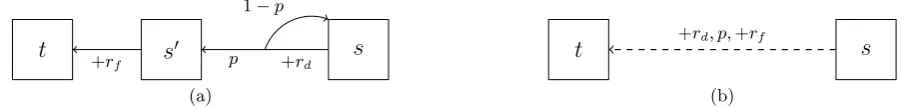
The appeal reduction gadget.
exponential-time lower bound for Dantzig’s rule [17], and by Fearnley to show an exponential-time lower bound against the all-switches rule [7].
The gadget is shown in Figure 1. Throughout the paper, we will use the following diagramming notation for MDPs. States are represented as boxes, and the name of the state is displayed in the center of the box. Each action is represented by an arrow that is annotated by a reward. If an action has more than one possible destination state then the arrow will split, and the reward is displayed before the split, while the transition probabilities are displayed after the split. The left half of Figure 1 diagram shows the gadget itself, and the right half shows our diagramming shorthand for the gadget: whenever we use this shorthand in our diagrams, we intend it to be replaced with the gadget in the left half of Figure 1. To understand the purpose of this gadget, imagine that
rf and rd are both 0. If this is the case, then we have the
following two properties. Letabe the action fromstos0.
• Ifσis a policy withσ(s) =a, then we have Valσ(s) = Valσ(t).
• Ifσis a policy withσ(s)6=a, and if Valσ(t) = Valσ(s)+ b, for some constantb, then we have Appealσ(a) =p·b.
The first property states that the appeal reduction gadget acts like a normal action fromstotwhen it is used by a pol-icy. However, the second property states that, if the action is not used, then the appeal of moving fromstotis reduced by the probabilityp. In short, an appeal reduction gadget can be used to make certain actions seem less appealing. Since Dantzig’s rule always switches the action with highest appeal, this will allow us to control which action is switched. The rewardsrf and rd give us further control on precisely
how appealing the action is, and how rewarding the action is when it is used by a policy.
Circuit iteration problems.
The starting point for ourPSPACE-hardness reductions will be a pair of circuit iteration problems. Acircuit iteration instance is a triple (F, B, z), whereF :{0,1}n→ {0,1}nis
a function represented as a boolean circuitC,B∈ {0,1}n
is an initial bit-string, andzis an integer such that 1≤z≤n. We use standard notation for function iteration: given a bit-stringB∈ {0,1}n
, we recursively defineF1(B) =F(B), and Fi(B) = F(Fi−1(B)) for all i > 1. We define two different circuit iteration problems, which correspond to the two different theorems that we prove for Dantzig’s rule. The problems are:
• BitSwitch(F, B, z): if the z-th bit of B is 1, then decide whether there exists an eveni≤2n such that
thez-th bit ofFi(B) is 0.
• CircuitValue(F, B, z): decide whether the z-th bit ofF2n(B) is 0.
The requirement forito be even inBitSwitchis a technical requirement that is necessary in order to make our reduction work. The fact that both of these problems are PSPACE -complete should not be too surprising, because we can use the circuitF to simulate a single step of a space-bounded Turing machine, so iteratingF simulates a run of a space-bounded Turing machine.
In order to make our reduction work, we must make sev-eral assumptions about the format of the circuit C, all of
which can be made without loss of generality. Firstly, we assume that the circuit only contains Not gates and Or
gates. Secondly, we make an assumption about gate depths. For each gatei, we used(i) to denote thedepth of the gate, which is the length of the longest path fromito an input bit. We assume that, for everyOrgate, both inputs of the gate have the same depth. Finally, we assume that the circuits are presented innegated form, which means that all of the output bits are negated. That is, the z-th output bit will produce a 1 if and only ifF(B) is 0. We also make several further technical assumptions about the precise format of the circuit, which are explained in detail in the full paper, but which are not necessary for a high-level understanding of how the construction works.
3.
THE CONSTRUCTION
Our main result is thatBitSwitch and CircuitValue can be reduced to ActionSwitch and DantzigMdpSol, respectively. Both reductions use the same construction, but the reduction fromCircuitValuetoDantzigMdpSol uses one extra gadget that we will describe at the end. Let (F, B, z) be a circuit iteration instance, and let C be the circuit that implementsF. In this section, we give a high-level overview of how our construction converts (F, B, z) into an MDP. A complete formal definition of our construction is available in the full version of the paper.
The construction is driven by aclock, which consists of a modified version of the exponential-time examples of Meleko-poglou and Condon [17]. The clock has two output states
c0 and c1, and the difference in value between these two
states is what drives our construction. In particular, the clock alternates between two output phases: in phase 0 we have Valσ(c
1) Valσ(c0), while in phase 1 we have
Valσ(c0)Valσ(c1). The clock alternates between phase 0
and phase 1, and goes through exactly 2nphases in total. The construction also containstwo full copies of the cir-cuit C, which we will call circuit 0 and circuit 1. At the start of the computation, circuit 0 will hold the initial bit-string B in its input bits. During phase 0, circuit 0 will compute F(B), and circuit 1 will copyF(B) into its input bits. The clock then moves to phase 1, which causes circuit 1 to computeF(F(B)), and circuit 0 to copyF(F(B)) into its input bits. This pattern is then repeated until 2nphases
have been encountered, and so when the clock terminates we will have computedF2n(B).
Each copy of the circuit is built from gadgets. We design gadgets to model the input bits,Orgates, andNotgates. In particular, for each gate i in the circuit, and for each
j ∈ {0,1}, there is a stateoji, which represents the output of the gateiin copyjof the circuit. The value of this state will indicate whether the gate is true or false. We use a family of constantsHk,Lk, andbk, which have the following
properties: for eachkwe haveHk> Lk,Hk=Lk+bk, and Hk=Lk+1. The idea is thatHk andLk give high and low
values, which will be used by gates of depth k to indicate whether they are true or false. More precisely, the truth values in circuitjwill be given relative to the value of the clock statecj. Given a policyσ, we say that:
• Gateiis false inσin phasejif Valσ(oji) = Val σ
(cj) + Ld(i).
s
s
0t
+rd p
1−p
+rf
(a)
s
t
+rd, p,+rf [image:5.595.79.531.67.121.2](b)
Figure 1: Left: The appeal reduction gadget with rewardsrf andrd, and probabilityp. Right: our shorthand for the appeal
reduction gadget.
Throughout this high-level description, we will use “gate
i outputs x” as a shorthand for saying that Valσ(oji) = Valσ(cj) +x.
We now describe the gadgets used in the construction. Throughout our exposition, we will only describe the parts of the construction that are necessary for understanding the high-level picture. In particular, we will not define the prob-abilities used in the appeal reduction gadgets, because know-ing the precise probabilities is not necessary for understand-ing the construction.
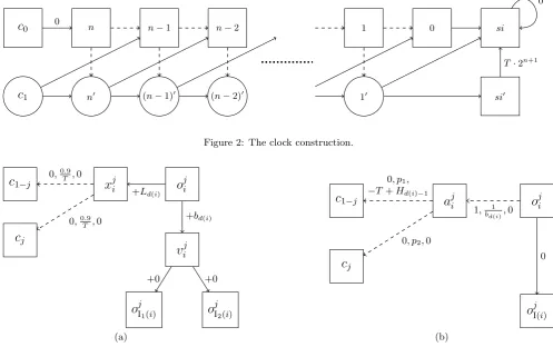
The clock.
Figure 2 shows the clock. We have used special notation to simplify this diagram. The circle states have a single out-going actiona. Each circle state has two outgoing arrows, which both have probability 0.5 of being taken when a is used. The clock is an adaptation of the exponential-time lower bound of Melekopoglou and Condon [17], but with several modifications. Most importantly, while they consid-ered minimising the reachability probability of state 0, we consider maximizing the expected total reward.
Note that the two statesc0andc1are the two clock states
that we described earlier. In the initial policy for the clock, all states select the action going right. In the optimal policy, all states select the action going right, except state 1, which selects its downward action. However, to move from the initial to final policy, Dantzig’s rule makes an exponential number of switches. In each step, the probability of reaching
si0 increases. The large payoff of T ·2n+1, where T is a large positive constant, ensures that the difference in value betweenc0 andc1is always T.
Or gates.
Figure 3a shows the gadget that will be used for eachOr
gateiin circuitj∈ {0,1}, where I1(i) and I2(i) are the two
inputs for gatei. As the circuit is computing in phasejwe will have thatxji takes the action towardscj. The behaviour
of this gadget is comparatively straightforward. If one of the two input gates outputs a high signal, then the statevijwill switch to the corresponding output state, and the output of gateiwill beHd(i)−1+bd(i) =Hd(i). On the other hand,
if both input gates output a low signal, thenoji will switch
to xji, so in this case the gate outputs Ld(i), which is the
correct output for this case.
Not gates.
Figure 3b shows the gadget that will be used to represent aNotgateiin circuitj∈ {0,1}, where I(i) is the input to the gate. The state aji is used to activate the gadget. At the start of clock phasej, we have thataji takes the action
towardscj. The probability p1 will be carefully chosen to
ensure thataji can only switch toc1−jafter the output of all
gates with depth strictly less thanihas been computed. The gate activates whenaji switches toc1−j. While the gadget
is not activated, the state oji will use the action towards
ojI(i). Once the gadget has been activated, there are then two possible outcomes, depending on whether the input bit is low or high.
• If the input bit is low, then the appeal of switching
oji to aji is large. So, oji will be switched to aji, and the rewards on the action from oji to aji and on the action from aji to c1−j ensure that the gate outputs Hd(i)−1+bd(i)=Hd(i), which is the correct output for
this case.
• If the input bit is high, then the appeal of switching
oji toaji is smaller, because the stateojI(i) has a higher value. In fact, we ensure that the appeal is so small that the action fromoji toaji will never be switched, because its appeal is smaller than the appeal of the action that advances the clock to the next phase. So,oji
never switches away fromojI(i), and therefore the gate will outputHd(i)−1=Ld(i), which is the correct output
for this case. Here we can see why the relationship betweenHd(i)−1 andLd(i) is needed in order for our
reduction to work.
Input bits.
Figure 4 shows the gadget that we will use for every in-put bit iand everyj ∈ {0,1}, where I(i) gives the output bit that corresponds to input biti. Since the input bits lie at the interface between the two circuits, they are the most complicated part of the construction. The input bit gadget has two distinct modes. During phase j, when circuit j is computing, the input bits in circuit j are in output mode, which means that they output the values that they are stor-ing. During phase 1−j, when circuitjis copying, the input bits in circuit j are in copy mode, which means that they must copy the output of gate I(i) from circuit 1−j.
We start by describing the output mode. In this mode, statesljiandrji both take the action towardscj. The output
is determined by the action chosen by stateoji: if the action tolji is chosen, then the gadget outputs the high signalH0,
and if the action to rij is chosen, then the gadget outputs
the low signalL0.
When the gadget is in copy mode, the statelij takes the action towardsc1−jand the staterji takes the action towards o1I(−i)j. In this mode, the state oji initially takes the action towards lji. If at any point the gate I(i) outputs a high signal, thenoji switches tor
j
c
0 n n−1 n−2 1 0 sisi0
c
1 n0 (n−1)0 (n−2)0 100
0
[image:6.595.54.552.73.385.2]T·2n+1
Figure 2: The clock construction.
v
jio
jI1(i)
o
j I2(i)
o
jix
jic
jc
1−j+0 +0
+bd(i)
+Ld(i)
0,0T.9,0 0,0.9
T ,0
(a)
o
jio
jI(i)a
jic
1−jc
j0 1, 1
bd(i),0
0, p1, −T+Hd(i)−1
0, p2,0
(b)
Figure 3: Left: The gadget for anOrgateiin circuitj. Right: A gadget for aNotgateiin circuitj.
signal, thenoji does not switch away fromlji. Hence, when the gadget moves back into output mode, it will output a high signal if and only if I(i) gave a low signal in the previous phase. Since we require that the circuit is given in negated form, this is the correct behaviour.
The most complicated part of the construction is ensur-ing that the input bits switch modes correctly at the end of each clock phase. This is difficult because we must ensure that the data held by the statesoji is not lost, and because
this operation happens simultaneously in both circuits. Ul-timately, we show that there are probabilitiesp3throughp7
that ensure that the mode transitions occur correctly.
ActionSwitch isPSPACE-complete.
We have now completed the high-level description of all of the gadgets in the construction. Suppose that we are given an instanceBitSwitch(F, B, z). We define an initial policyσinitsuch that the input bits in circuit 0 output the
bit-stringB. The stateo0z is the output state of the
input-bit gadget corresponding to the z-th input bit. When we execute Dantzig’s rule starting fromσinit, we have that the
state o0z switches to rz0 if and only if there exists an even i≤2nsuch that the z-th bit ofFi(B) is 1. So, we have a reduction fromBitSwitchtoActionSwitch, which proves thatActionSwitchisPSPACE-complete.
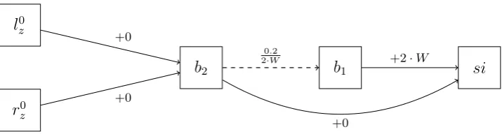
DantzigMdpSol isPSPACE-complete.
To show that DantzigMdpSol is PSPACE-complete, we
use one additional gadget, which is shown in Figure 5. Sup-pose that we have an instanceCircuitValue(F, B, z). We create the MDP as before, but the additional gadget in-terfaces with the states l0
z and r0z from the z-th input bit
gadget. The purpose of this gadget is to make sure that the
z-th output bit computed in phase 2n is not destroyed by any subsequent switching.
In the initial policy, the stateb2uses the action that goes
directly to the state si from the clock. In this configura-tion,b2 has value 0, so the states l0z andr0z will not switch
to b2. Therefore, the behaviour of policy iteration will be
unchanged, and Dantzig’s rule will computeF2n(B). The appeal reduction gadget betweenb2 andb1 is
config-ured so that b2 switches tob1 immediately after the 2n-th
clock phase. Once this has occurred, the stateb2 will have
value 2·W, where the payoffW is chosen to be extremely large, so bothl0
z andr0z will switch tob2. After both states
have switched, the state o0z will be indifferent between its
two successors, so it can never be switched. Thus, when policy iteration terminates with an optimal policy, the ac-tion chosen by o0z will be determined by the z-th bit of F2n(B), which completes the reduction fromCircuitValue
toDantzigMdpSol.
4.
CONCLUSION
o
jil
ijr
ijo
1I−j(i)c
1−jc
j0, p3,0
0, p5,−T2 +
Hd(C)+Ld(C) 2
0, p4, H0 0, p6, L0
0, p7,−T2
[image:7.595.148.464.50.203.2]0
Figure 4: The gadget for input bitiin circuitj.
si
b
1b
2l
0 zr
z00.2
2·W +2·W
+0 +0
+0
Figure 5: The extra gadget needed in Constr(C, z).
might be to consider Bland’s rule, which assigns an index to each variable, and always pivots the variable with negative reduced cost that has the least index. It is possible that our construction might be applied in a rather direct way to show results for Bland’s rule, since our construction essentially relies on controlling the order in which actions are switched in the MDP.
Providing results for other pivot rules will probably be more challenging, and require different constructions. The steepest edge pivot rule is the one that is most commonly used in practice, so provingPSPACE-completeness results for this rule might be the next logical step. It is not even known if the steepest edge switching policy can take exponential time for MDPs. There are also other rules, such as the one that in each step gives the biggest overall improvement in the objective function, where PSPACE-completeness results would be interesting.
Moving away from linear programming, our results in-dicate that we may be able to show PSPACE-completeness results for a wide variety of different algorithms. As men-tioned in the introduction, this type of result was only pre-viously known to hold for algorithms that solvePPAD-hard or PLS-hard problems, but our results indicates that this phenomenon may be more widespread. In particular, par-ity games, mean-payoff games, and discounted games are three problems that lie at the intersection ofPPADandPLS, but which are not known to lie in P. Strategy improve-ment algorithms, which are a generalisation of policy iter-ation, are used to solve these games, and these algorithms are an obvious target. Note that our results already hold for strategy improvement algorithms that solve stochastic mean-payoff games, because these games are a superset of
average-reward MDPs. It seems likely that this can be used directly to show results for stochastic discounted games, and simple stochastic games, using reductions similar to the ones used by Friedmann in the non-stochastic setting [9].
Another target might be Lemke’s algorithm for solving linear complementarity problems (LCPs). For the special case ofP-matrix LCPs, the problem of finding a solution is known to lie at the intersection of PPAD and PLS, but not known to lie in P. At first glance, such results may not seem possible for P-matrix LCPs, because these problems are known to always have a unique solution. However, there is some leeway for a result here, because the solution can lie at the boundary between multiple convex cones, and the algorithm will only return one of these cones as a solution.
Ultimately, the end goal of this line of research is to pro-duce a “recipe” for PSPACE-hardness than can be applied to a wide variety of simplex pivoting rules. For example, Adler, Papadimitriou, and Rubintstein ask whether such a result holds for all pivoting rules that use only primal feasible bases [2]. Any such recipe would shed light on the require-ments for a strongly polynomial-time pivot rule. While we believe our work has made an important first step, it is clear that much further research will be necessary to achieve this goal.
5.
ACKNOWLEDGEMENTS
This work was supported by EPSRC grant EP/L011018/1 “Algorithms for Finding Approximate Nash Equilibria.”
6.
REFERENCES
[image:7.595.127.485.234.330.2]quadratic functions of the smaller dimension.J. ACM, 32(4):871–895, Oct. 1985.
[2] I. Adler, C. Papadimitriou, and A. Rubinstein. On simplex pivoting rules and complexity theory. InProc. of IPCO, 2014.
[3] K. H. Borgwardt.A Probabilistic Analysis of the Simplex Method. Springer-Verlag New York, Inc., New York, NY, USA, 1986.
[4] X. Chen, X. Deng, and S.-H. Teng. Settling the complexity of computing two-player Nash equilibria. J. ACM, 56(3):14:1–14:57, May 2009.
[5] G. B. Dantzig.Linear programming and extensions. Princeton University Press, 1965.
[6] Y. Disser and M. Skutella. In defense of the simplex algorithm’s worst-case behavior.CoRR,
abs/1311.5935, 2013.
[7] J. Fearnley. Exponential lower bounds for policy iteration. InProc. of ICALP, pages 551–562, 2010. [8] O. Friedmann. An exponential lower bound for the parity game strategy improvement algorithm as we know it. InProc. of LICS, pages 145–156, 2009. [9] O. Friedmann. An exponential lower bound for the
latest deterministic strategy iteration algorithms. Logical Methods in Computer Science, 7(3), 2011. [10] O. Friedmann. A subexponential lower bound for
Zadeh’s pivoting rule for solving linear programs and games. InProc. of IPCO, pages 192–206, 2011. [11] O. Friedmann, T. D. Hansen, and U. Zwick. A
subexponential lower bound for the random facet algorithm for parity games. InProc. of SODA, pages 202–216, 2011.
[12] O. Friedmann, T. D. Hansen, and U. Zwick.
Subexponential lower bounds for randomized pivoting rules for the simplex algorithm. InProc. of STOC, pages 283–292, 2011.
[13] P. W. Goldberg, C. H. Papadimitriou, and R. Savani. The complexity of the homotopy method, equilibrium selection, and Lemke-Howson solutions.ACM Trans. Economics and Comput., 1(2):9, 2013. Preliminary version: FOCS 2011.
[14] T. D. Hansen, H. Kaplan, and U. Zwick. Dantzig’s pivoting rule for shortest paths, deterministic MDPs, and minimum cost to time ratio cycles. InProc. of SODA, pages 847–860, 2014.
[15] D. S. Johnson, C. H. Papadimitriou, and
M. Yannakakis. How easy is local search? J. Comput. Syst. Sci., 37(1):79–100, 1988.
[16] V. Klee and G. Minty. How good is the simplex algorithm? InInequalities, III, pages 159–ˆa ˘A¸S175, 1972.
[17] M. Melekopoglou and A. Condon. On the complexity of the policy improvement algorithm for Markov decision processes.INFORMS Journal on Computing, 6(2):188–192, 1994.
[18] B. Monien and T. Tscheuschner. On the power of nodes of degree four in the local max-cut problem. In Proc. of CIAC, pages 264–275, 2010.
[19] C. H. Papadimitriou, A. A. Sch¨affer, and
M. Yannakakis. On the complexity of local search. In Proc. of STOC, pages 438–445, 1990.
[20] I. Post and Y. Ye. The simplex method is strongly
polynomial for deterministic Markov decision processes. InProc. of SODA, pages 1465–1473, 2013. [21] M. L. Puterman.Markov Decision Processes: Discrete
Stochastic Dynamic Programming. John Wiley & Sons, Inc., New York, NY, USA, 1st edition, 1994. [22] A. A. Sch¨affer and M. Yannakakis. Simple local search
problems that are hard to solve.SIAM J. Comput., 20(1):56–87, 1991.
[23] S. Smale. On the average number of steps of the simplex method of linear programming.Mathematical Programming, 27(3):241–262, 1983.
[24] S. Smale. Mathematical problems for the next century. The Mathematical Intelligencer, 20(2):7–15, 1998. [25] D. A. Spielman and S.-H. Teng. Smoothed analysis of
algorithms: Why the simplex algorithm usually takes polynomial time.J. ACM, 51(3):385–463, May 2004. [26] M. Yannakakis. Computational complexity. In