Application of a coastal modelling code in fluvial environments

promoting access to White Rose research papers

White Rose Research Online [email protected]

Universities of Leeds, Sheffield and York

http://eprints.whiterose.ac.uk/

This is an author produced version of a paper published in Environmental Modelling and Software.

White Rose Research Online URL for this paper:

http://eprints.whiterose.ac.uk/43670/

Paper:

Hartanto, IM, Beevers, L, Popescu, I and Wright, NG (2011) Application of a coastal modelling code in fluvial environments. Environmental Modelling and Software, 26 (12). 1685 – 1695.

1

XBeach: Application of a Coastal Modelling Code in Fluvial Environments

I.M. Hartanto a, L. Beevers a, I. Popesccu a,*, N.G. Wrightb

a

UNESCO-IHE Institute for Water Education, P.O. Box 3015, 2601 DA, Delft, The Netherlands; FAX (31) 15-3122921, e-mail:[email protected]; [email protected]; [email protected]

b

University of Leeds, Leeds LS2 9JT,United Kingdom , e-mail:[email protected]

* _{Corresponding author:}

[email protected] (I. Popescu), P.O. Box 3015, 2601 DA, Delft, The Netherlands; FAX (31) 15-3122921, TEL(31) 15 2151895

Abstract

XBeach is an open source, freely available two-dimensional code, developed to solve

hydrodynamic and morphological processes in the coastal environment. In this paper the code is applied to ten different test cases specific to hydraulic problems encountered in the fluvial environment, with the purpose of proving the capability of XBeach in rivers. Results show that the performance of XBeach is acceptable, comparing well to other commercially available codes specifically developed for fluvial modelling. Some advantages and deficiencies of the codes are identified and recommendations for adaptation into the fluvial environment are made.

Keywords: Numerical model, River System, XBeach, Shallow Water Equations, Open Software

1 Introduction

Historically coastal modelling software has developed out of different constraints from fluvial software, due to the necessity of representing different characteristics of hydraulic behaviour. Parameters like wind and tidal forces, which have high influence in the coastal environment (de Vriend, 1991), have minor effects in fluvial environments. Conversely, a longitudinal slope and varying initial water level, which are very important in river modelling, are not considered important in coastal modelling. However, the hydraulic calculations are similar, hence coastal software can be applied in fluvial areas. The application of a code outside its original domain needs to be verified and tested comprehensively before wider application is attempted.

2

calculate a fluvial flood wave. Open source codes provide payment-free software (usually under the GNU Public License - http://www.gnu.org/licenses/gpl.html) to users, which is a key

advantage in developing countries (Bitzer, 2004; Lanzi, 2009). This approach allows the user to modify the code to meet their specific requirements (Henley and Kemp, 2008) and can lead to a significant development and improvement of the code, whilst affording flexibility.

This research tests the validity of applying this freely available software in a cross-over domain (fluvial environments), which opens up its use to a greater number of professionals, and also permits use in coastal/river transition zones such as estuarine areas. Due to the morphological tools available within the software, specialists would also have the possibility of accessing free 2D sediment transport capabilities. XBeach has generally been used as a stand-alone model for small scale coastal applications. It has many capabilities such as: depth-averaged shallow water equations including subcritical and supercritical flow, time-varying wave action balance, wave amplitude effect and the depth-averaged advection-diffusion equations (Roelvink et al. 2009). This paper focuses solely on the depth-averaged shallow water equations solver.

The main objective of the development of the XBeach was to provide modellers with a robust and flexible environment where the concepts of dune erosion, over washing and breaching can be tested (Roelvink et al. 2009). During the code development, the stability of the numerical method was considered as a top priority. Consequently, first order accuracy was accepted since the software concentrated on representing near shore and swash zone processes which have strong gradients in time and space (Roelvink et al. 2008). Such accuracy is the norm in river modelling software.

3

2 Theoretical background

2.1 Numerical methods

The increased demand for improved safety against flooding, prompted the development of mathematical models which describe flow propagation in rivers. These mathematical models, in most cases, do not have an analytical solutions and are solved using numerical methods. Flow description in rivers, lakes and coasts are long waves, which can be described by means of the so-called Shallow Water Equations. These are a hyperbolic set of partial differential equations depending on the nature of the problem to be solved. These equations describe the mass conservation and momentum conservation.

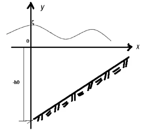
Significant effort during the 1980’s and 1990’s was devoted to defining efficient and accurate numerical methods for hyperbolic systems. Mathematically the hyperbolic equations permit discontinuous solutions and their numerical integration should lead to the computation of such discontinuities sharply and without oscillations.

4

The differential form of the Shallow Water equations, in the reference framework of figure 1, are:

(1)

Where:

is the domain of computation;

σ is any open subset of with boundary Г

n is the outward unit normal

The vectors included in the equation are:

(2) 

With q(x,t) - the unit-width discharge,

ho(x, y) - the depth under the reference plane in figure 1,

ζ( ( x , y, t ) - the elevation over the same reference plane, h(x, y, t) = ho + ζ

g - the gravitational acceleration

s - the source term which accounts for the bottom slope

Г is the boundary of σ.

B and C the Jacobian matrices of the fluxes f and g respectively.

Equations (2) are the conservative form of the Shallow Water equations (all the spatial derivatives of the unknowns are in the form of a divergence operator). In the case of a flat bottom (ho = 0) the right-hand side of the equation is 0 and the equation is the strong conservation form of the Shallow Water equations.

5

equations are equivalent to one another if the solution belongs to C. This equivalency is no longer valid when shocks (i.e. bores) are involved.

Current codes which solve the Shallow Water equations do so using different numerical methods. From the current literature, several numerical techniques for solving the Saint Venant Equations are available. These include the method of characteristics, explicit difference methods, semi-implicit methods (Casulli, 1990), fully implicit methods, and Godunov methods (van Leer, 1979). The characteristic method transforms the Shallow Water partial differential equations into a set of ordinary differential equations, which are solved using finite difference methods. The explicit methods transforms the Shallow Water equations into a set of algebraic equations, which can be solved, in sequence, at each point of discretisation, at each time step, while implicit methods solve the equations simultaneously at all computational points at a given time. If, due to boundary conditions and assumptions, the set of Shallow Water equations are non-linear, iteration is needed in order to find the solution.

Numerical stability and convergence issues need to be addressed, while solving the Shallow Water equations numerically. In order to prevent error propagation in explicit methods, the Courant Frederichs Levy (C.F.L.) condition is imposed. This relates the time step to the spatial discretization and the wave speed, i.e. the time step must be less than or equal to the ratio of the

reach length to the minimum dynamic wave celerity ( .

Godunov-type methods can be explicit or implicit. Generally, however, they are explicit in time and, accordingly, the allowed time step is restricted by the C.F.L. stability condition. These methods are in general based on non-staggered grids and can achieve first-order accuracy. Godunov-type methods were originally developed for gas dynamics and were then later extended to hydrodynamics on the basis of the analogy between the equations for isentropic flow of a perfect gas with constant specific heat and the Shallow Water Equations. (Toro, Leveque)

6

the conservation of both fluid volume and momentum then problems addressing rapidly varying flow can be solved. (Stelling and Duinmeijer, 2003).

There are a number of different numerical schemes embedded in different codes, for example: the weighted four point-Preissmann scheme (Preissmann 1960), Godunov-based methods (LeVeque 1992), the the weighted six-point Abbott-Ionescu scheme (Abbot and Ionescu 1967), and TVD (Total Variation Diminishing) schemes (Toro 1997). Each numerical scheme has its own advantages and disadvantages. Below schemes relevant to this paper are discussed.

The first schemes developed for hydrodynamic computational codes were the fully implicit schemes of Preissmann and Abott–Ionescu during the 1960s. These schemes have developed over time (most significantly in terms of graphical user interfaces GUI), but remain the most popular and widely used in commercially available software. Two examples of codes that use the Preissmann scheme are DAMBRK, which was developed by the US National Weather Service, and ISIS which was developed by Halcrow and HR Wallingford in the UK. An example of a code using Abbott-Ionescu scheme is Mike11, developed at Danish Hydraulic institute.

Godunov developed a method to solve the non-linear systems of the hyperbolic conservation laws describing fluid flow. As a result, the scheme is able to solve the Riemann problem by including various approximate Riemann solvers (Toro 1997). The Riemann problem is a

discontinuity of the conservation law and of piecewise constant data (LeVeque 1992). Godunov-based schemes with various Riemann solvers are used in river modelling software such as Infoworks RS 2D (Roca and Davison 2009), TRENT (Villanueva and Wright, 2006) and BreZo (Begnudelli et al., 2008).

7

Finally , XBeach uses the Stelling and Duinmeijer scheme (Stelling and Duinmeijer 2003), combining the efficiency of staggered grids with momentum conservation properties needed to ensure accurate results for rapidly varied flows and expansion and/or contractions. This method is very efficient in simulating large scale inundation (Stelling and Duinmeijer 2003).

2.2 XBeach formulation

XBeach uses a rectilinear, non-equidistant, staggered grid. This discretisation calculates bed level, water level, water depth and concentration of sediment at cell centres while velocities and sediment transport are calculated at the cell border. Velocities at the cell centres are obtained by interpolating the results from the four surrounding points (Roelvink, et al., 2009).

The shallow water equations that are used in XBeach are two dimensional, non-conservative, and are as follows:

Continuity:

0

hu hv

t x y

η

∂ ₊∂ ₊∂ ₌

∂ ∂ ∂ (3)

X momentum:

2 2

2 2

sx bx x

h

F

u u u u u

u v f v g

t x y x y h h x h

τ τ η

ν

ρ ρ ρ

⎛ ⎞

∂ ₊ ∂ ₊ ∂ _{− −} ∂ ₊∂ _{= − −} ∂ ₊

⎜ ⎟

∂ ∂ ∂ _⎝∂ ∂ _⎠ ∂ ₍₄₎

Y momentum:

2 2

2 2

sy by y

h

F

v v v v v

u v f u g

t x y x y h h y h

τ τ η

ν

ρ ρ ρ

⎛ ⎞

∂ ₊ ∂ ₊ ∂ _{+ −} ∂ ₊∂ _{= + − −} ∂ ₊

⎜ ⎟

∂ ∂ ∂ _⎝∂ ∂ _⎠ ∂ (5)

Here τbx, τby are the bed shear stresses, η is the water level, Fx, Fy are the wave-induced stresses,

νt is the horizontal viscosity and f is the Coriolis coefficient (Roelvink et al. 2009). The other notations in the equations are:

η = water level

t = time

8 u,v = water velocity

f = Coriolis coefficient

ρ = water density

g = gravity force per unit mass

νt = horizontal viscosity h= water depth

τbx, τby = bed shear stresses Fx, Fy = wave-induced stresses

A first order upwind explicit schematisation with an automatic time step is the preferred numerical method used in XBeach (Roelvink et al, 2003), due to the many shock-like characteristics which occur in hydrodynamic and morphodynamic behaviour (Stelling and Duinmeijer 2003). The discretisation is similar to the one developed by Stelling and Duinmeijer in its momentum-conserving form, hence it is able to capture shocks and is very suitable for 'drying and flooding', allowing for combinations of sub- and supercritical flows.

The developers of XBeach selected upwind scheme in order to avoid numerical oscillations of many shock-like phenomena, which occur in coastal and flooding situations. . The scheme is able to avoid shock oscillations introduced by the additional dissipative term (Hibberd and Peregrine 1979). As a result, the upwind scheme, together with a staggered grid, makes the model robust (Roelvink et al., 2009).

9

Table 1: Summary of tests completed

Test no. Name Description Figure no.

1a,1b

1c, 1d

Semi-analytical Comparison of the model runs with semi-analytical solutions. M1, M2 curves (mild slope);

S2, S3 curves (steep slope)

Fig. 2, 3

2a

2b

2c

Idealised Flow in a straight idealised channel

Flow in an embanked straight idealised channel Flow in a meandering idealised channel

Fig. 4

Fig. 5

3 EA case 1 Wetting and drying of a disconnected body Fig. 6a & 6b

4 EA case 2 Low momentum flow Fig. 7

5 EA case 3 Momentum conservation Fig. 8

6 EA case 4 Flood propagation over a plain Fig. 9 & 10

7 EA case 5 Dam break over a valley Fig. 11 & 12

8a

8b

EA case 6 IMPACT: Hydraulic jump and wake zone (laboratory scale) IMPACT: Hydraulic jump and wake zone (realistic scale)

Fig. 13 Fig. 14

9 Experimental Dam break through an urban area Fig. 15

3 Test cases

3.1 Semi-analytical solution comparison

There are certain fluvial hydraulic scenarios which can be solved using semi-analytical methods. These cases provide the starting point for testing the capability of XBeach in the fluvial

environment. In addition to the cases that have semi-analytical solutions, there are also cases where known fluvial behaviour can be tested.

The first test examines XBeach’s capability to model simple cases such as gradually varied flow and backwater effects, Test 1a-d. The code was tested to model mild slope types (M1 and M2) and steep slope types (S2 and S3) (Chow 1959; Cunge et al. 1980).

10

constant 5 m water level boundary condition in downstream. These conditions at the boundaries generate a M1 flow curve which varies from a water level of 1.17 m to 5 m.

The M2 flow curve (Test 1b) was set up using a 5 m3/s/m discharge at the upstream boundary and a critical depth of 1.37 m at the downstream boundary of the model. These boundary conditions generate a normal water depth of 2.15 m at the upstream boundary.

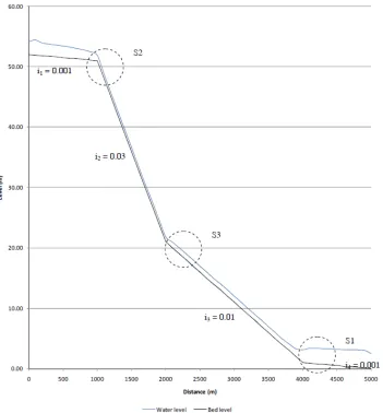
The cases 1c and 1d are the steep slope cases, here the S2 and S3 flow curves are generated using a 5 km long channel with various bed slopes (i.e. 0.03, 0.01 and 0.001), as shown in Figure 2. The upstream boundary condition is set as a constant discharge of 5 m3/s/m, and the downstream boundary condition of 2.15 m water level. The S2 flow curve occurs after the transition from the 0.001 to the 0.03 slope and the S3 flow curve at the transition from 0.03 to 0.01 slope.

11

The second theoretical case (Test 2a) is a straight trapezoidal channel with a flat floodplain on both sides. The model uses a uniform value of Chézy roughness coefficient for both the main channel and floodplain area. The test investigates the two dimensional flow calculations of the software. Furthermore, Test 2b investigates the case of an embanked floodplain to examine the hydraulic representation of a disconnected waterbody.

Case 2a was modelled using a 5 km long, straight channel, with a 0.001 slope and a river cross-section of 30 m width (bottom), 2 m deep and floodplain of 30 m each side. The upstream boundary condition was a varying discharge from 50 to 700 m3/s with the peak discharge occurring after 43.3 minutes and a minimum value after 60 minutes. The dimensions of the channel were set so as to allow an overflow at the peak flow. In Case 2b dikes are constructed on both banks of the channel.

12

More complex, and realistic, hydraulic behaviours throughout the domain are found in

meandering channels. A perfect sinusoidal meander with no slope was modelled (Test 2c). This test investigates the water flows from the main channel to floodplain and vice versa, secondary flow in the curved channel and velocity distributions as well as flood wave behaviour.

For Case 2c the modelled reach uses a rectangular channel 50 m wide and 5 m depth, with a length of 4.50 km. The actual model domain was only 3km as the meanders were introduced to create the extra length in the main channel. The total width of the floodplain was 600m on both river banks. A zero bed slope was applied in this case, in order to model flow in the channel only as a result of the upstream boundary condition. This was set as a varying discharge (from 200 m3/s to 1000 m3/s),

3.2 The Environment Agency 2D Benchmarking Study (EA2D)

In 2009, the Environment Agency of England and Wales carried out a benchmarking study for 2D software. The benchmarking was undertaken to ensure that codes used for fluvial studies commissioned by the Agency were appropriate for use in assessing flood risk. The project was led by Heriot Watt University (Heriot-Watt 2009) and the simulations were set up and carried out by various model developers throughout the world. The final report of this study is available to the public (Neelz and Pender, 2010). Six out of eight EA2D tests were chosen to test the ability of XBeach in fluvial modelling situations. For this study comparisons were made to InfoWorks RS 2D and ISIS 2D.

13

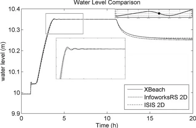
Test 4 determines inundation extent with low momentum flows in a complex topography. Furthermore, it also examines the disconnected water body, wetting and drying of a floodplain, inundation extent and looks at final depth rather than maximum depth. The model domain is a sloped plain in two directions with 16 depressions included in the terrain to retain a portion of the water that flows in from upper corner of the domain. The model covers an area of 2000 m x 2000 m with 16 depression each of 0.5 depth. There is an overall slope of 1:1500 in the north direction and 1:3000 towards the east, resulting in a ~2 m drop of elevation between top left corners to bottom right corner.

The inflow boundary condition was located at the top left side of the domain over a length of 100 m, with a discharge value of 20 m3/s for a period of 75 minutes starting at time t=10 minute. All other boundaries of the domain are closed boundaries.

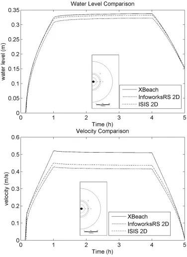
The fifth test simulates momentum flow over a barrier. This capability is important in sewer or pluvial flood modelling in urban floodplain areas. The domain consists of a steep slope to accelerate the inflow and a bump to disconnect it from another depression. The boundary condition is a discharge of 65.5 m3/s for 10 seconds starting at time t=5 s with a peak at time t=15. The model is 300 m long with a bump of 25 cm height. The domain consists of a steep slope to accelerate the inflow and a bump to disconnect it from another depression. The volume of the inflow is just enough to fill the depression. Water is expected to overtop the bump due to the force of momentum and settle in the depression behind the bump. This test differentiates codes which incorporate the full momentum terms and those that do not.

Case 6 tests the simulation of flood propagation over a wide floodplain following a dike failure. A high burst inflow is applied at the breach point, and a wide flat floodplain is modelled to test the propagation of a flood wave and velocities at the leading edge of the flood wave. The

modelled area is a 1000 m x2000 m of flat topography. The inflow boundary condition reaches a peak discharge of 20 m3/s at time t=60 mins and continues constantly with this value for a further 180 minutes. The inflow is located in the centre of the left boundary of the model. The objective of the test is to examine the capability of XBeach to simulate the speed of flood wave

14

The penultimate EA2D test (Test 7) models the simulation of a flood wave propagation

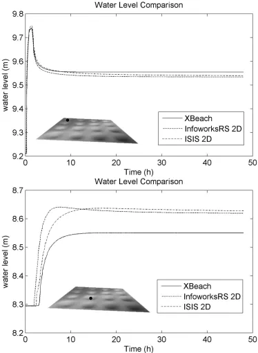
following a dam failure that flows through a river valley. The case tests the software’s capability in simulating major flood inundation and flood hazard prediction that arises from a dam break scenario. The software was expected to be able to model a high burst discharge over steep and mild bed slopes involving both subcritical and supercritical flow. The test has a skewed discharge boundary with peak flow of 3000 m3/s at time t=10 min for 10 minutes and slowly decreases thereafter for a further 80 minutes.

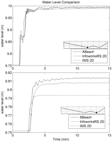
Test 8 is adapted from a benchmark test case from the IMPACT project (IMPACT 2005; Soares-Frazao and Zech 2002). This test examines the capability of the software to simulate hydraulic jumps and the wake zone behind a building. The test consists of two cases, the laboratory scale (1:20) (Test 8a) and the realistic scale (Test 8b). The scale of the scaled model is 1:20. The dam size is 3.6 m x 99 m with a breach of 1 m wide in the middle of the dam (6.75m from the left side of the dam). The initial water level in the reservoir behind the dam is 0.20 m, while the water level in the floodplain area is set to a value of 0.02 m (a wet bed domain). A model of a building is set in the floodplain in line with the dam breach location. Test 8b is a dam break case at real scale. The size of the computer model is obtained by multiplication with 20. Therefore the initial water level at the dam is 8.00 m and in the floodplain area is 0.4 m

3.3 Experimental case comparison

15

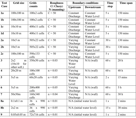
Details on the models meshes, sizes and boundary condition types are given in table 2. The Courant number used is not included in the table, but remains the same for all tests. The number used is 0.9.

Table 2.

Test Case

Grid size Grids counts

Roughness C( Chezy) N (manning)

Boundary conditions Time

step

Time span Upstream Downstream

1a 100x100 m 100x2 cells C = 50 Constant

Discharge Constant Water Level 5 s 150 mins

1b 100x100 m 100x2 cells C = 50 Constant

Discharge Constant Water Level 5 s 150 mins

1c 10x10 m 400x11 cells C = 50 Constant

Discharge

Constant Water Level

5 s 150 mins

1d 10x10 m 400x11 cells C = 50 Constant

Discharge Constant Water Level 5 s 150 mins

2a 10x5 m 505x22 cells C = 50 Varying

Discharge Constant Water Level 30 s 130 mins

2b 10x5 m 505x22 cells C = 50 Varying

Discharge Constant Water Level 30 s 130 mins

2c 100x100 m 598x133

cells

C = 50 Varying

Discharge

Constant Water Level

5 s 150 mins

3 2x2 m

(10x10 for other soft.)

350x50 cells n = 0.03 Varying Water Level

N/A (wall) 60 s 20 h

4 20x20 m 100x100

cells n = 0.03 Varying Discharge N/A (wall) 60 s 48 h

5 5x5 m 60x20 cells n = 0.05 Varying

Water Level

N/A (wall) 2 s 15 mins

6 5x5 m 200x400

cells n = 0.05 Varying Discharge N/A (wall) 60 s 5 h

7 50x50m 160x340

cells n = 0.04 Varying Discharge N/A (wall) 60 s 30 h

8a 0.1x0.1 m 36 x 990

cells

n = 0.01 N/A (initial water level) 1 s 2 mins

8b 2x2 m 36 x 990

cells n = 0.05 N/A (initial water level) 15 s 30 mins

9 0.05x0.05 m 72x716 cells n = 0.01 N/A (initial water level) 1 s 2 mins

4 Results and Discussion

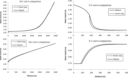
For the backwater cases comparing the modelled results with the semi-analytical results shows deviations (Figure 3). In the M1 and M2 cases, a difference is observed at the boundary while

16

steep slope (M2, S2), while smaller differences are observed at the transition from steep to mild slope (M1, S3). This is due to the transition from subcritical to supercritical flow and shows the ability of the code to capture shocks. Boundary conditions also show inconsistencies. The inconsistency in results observed at the boundary is due to the implementation of a flow boundary condition, which is currently represented using velocity vectors. These are implemented at the centre of each cell situated in the boundary.

17

Figure 4. Test 2a and 2b, Stage discharge in straight channel

18

For Test 3, the incoming water is expected to fill the depressions in the domain. Figure 6a and 6b shows that XBeach compares well with ISIS 2D and Infoworks RS 2D for this test. A small instability can be observed following maximum depth, on the downslope of the first bump (Figure 6a). Each computational code compared gives marginally different results. Additionally, differences are observed at initial and final water depths, which are of the order of a few

millimetres. In general however, the results of Test 3 show a good comparison to other fluvial computational codes.

Figure 6a. Test 3 - wetting and drying of a disconnected body (results recorded on the downslope of the initial bump)

19

On the other hand, Figure 7 shows the results of Test 4, where significant differences between codes can be observed. Due to the wet/dry threshold value that was set in XBeach, a greater number of dry depressions are observed than anticipated. The closer to the inflow location that the result is sampled the more favourable the XBeach comparison with other codes. However XBeach performs poorly in this test. The reason for this behaviour is that the threshold value of the wetting and drying algorithm is high. This means the domain retains 2 cm of water when it should actually be dry. This is due to the mathematical formulation of the problem whereby for Manning’s equation the depth (d) calculation is completed with the Manning coefficient located in the denominator and hence the expression generates errors. The problem could be avoided if the Chézy equation is used instead of Manning. The use of the Manning equation was due to the test requirements where the Manning model is the preferred roughness representation in the fluvial environment for the Environment Agency. This issue can be neglected when modelling real rivers, since the 2 cm threshold does not impact significantly at the larger scale.

20

21

22

23

24

25

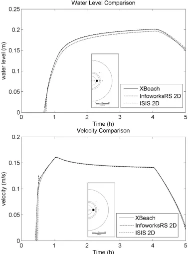
For the realistic scale dambreak test (Test 7), XBeach gives a higher final water level result than the other tested codes and a lower value for flow velocities for nodes located at the head of the valley (Figure 11). This trend is less evident further down the valley (Figure 12). This is

explained by the fact that Xeach is using a first order scheme, which is dissipative. However, for Test 8a (the EA2D laboratory small scale model), where the code’s ability to reproduce

hydraulic jumps at a laboratory scale is investigated, noticeable differences between the three codes for computed water depth and velocities can be seen (Figure 13). When this is translated into the realistic scale (Test 8b) however, a similar result is observed for all three codes (Figure 14).

The result from the dam break case through a valley (Test 7), and dam break over a building (Test 8b) gives comparable results to InfoWorks RS 2D and ISIS 2D. However, the small scale results show poor agreement (Test 8a), which is to be expected. Nevertheless, if Froude scaling is applied between the small scale measurement and simulation real scale computations for XBeach, a good match is found , which cannot be said for the other codes.

Finally, for Test 9, the comparison between XBeach and measured laboratory results of a dambreak experiment over an urban area shows large differences between the two, especially at the street level. Improved results are likely if the computational mesh were to be refined

significantly, however computational time would increase. This modification on the scale required however would be difficult. The structured rectangular grid that is used in XBeach can lead to a large number of cells, if it is applied to a detailed complex system at real-scale such as a meandering channel, bifurcation or an urban area, however it gives a quick solution when

26

27

28

29

Figure 15.Test 9 - Laboratory experiments

6 Conclusions

The Shallow Water equation solver in XBeach has been seen to work well for river modelling scenarios, when compared to other codes developed for the fluvial environments. Furthermore, with an open source licence, any user may improve the software or add flexibility. However, some deficiencies are acknowledged. The existing representation of the boundary conditions, while adequate for coastal environments, was not always applicable for fluvial modelling purposes, especially in the case of upstream flow conditions. A small sub-routine was implemented, however further refinement is warranted.

30

The assumption under which the Shallow Water equations are solved using Xbeach restricts application of these equations for flow problems with a steep bed slope, particularly for the supercritical cases. Consequently testing spillways with this code would imply changes were implemented so that supercritical cases can be tested as well. Pipe flow was not tested in this study.

Codes treating coastal problems address the wetting and drying of computational cells differently from 2D river modelling which result in different inundation patterns. This can be overcome by imposing a different threshold value than that used in coastal applications of XBeach. Similarly in the coastal environment Chézy is the roughness representation of choice. Transferring to the fluvial environment for this study requires the implementation of a subroutine to change the roughness coefficient, in this case to Manning’s. Further modification should be implemented.

XBeach uses a structured staggered grid which can be inflexible for representing complex fluvial geometries. As a recommendation for further development of XBeach, it is suggested that an unstructured grid option is investigated so as to avoid very fine grids.

Finally, the conclusion of this research opens up the possibility to use this model for both hydraulic and potentially morphological problems in fluvial, coastal and hence transition areas.

Acknowledgements

The authors would like to acknowledge the Environment Agency of England and Wales and Herriot Watt University for providing the EA2D test cases, and Wallingford Software (now MWH Soft) and Halcrow for providing their comparison data. Additionally the first author is grateful to the Dutch Development Co-operation Programme and to the Dutch StuNed

31

References

Abbot, M. B., Ionescu, F., 1967. On the numerical computation of nearly-horizontal flows. J. Hydraul. Res., 5(2), 97-11.

Ambrosi, D., 1995, Approximation of the shallow water equations by Roe’s Riemann solver. Int.Journal Of Num.meth.In Fluids, vol 20, p157-168

Begnudelli, L., Sanders, B. F. , Bradford, S. F. , 2008. Adaptive Godunov-Based Model for Flood Simulation. J. Hydraul. Eng. 134(6): 714-725.

Bitzer, J., 2004. Commercial versus open source software: the role of product heterogeneity in competition. Econ. Syst., 28(4), 369-381.

Chow, V. T., 1959. Open-channel hydraulics, MCGraw-Hill, New York.

Casulli, V, 1990, Semi-implicit finite difference methods for the two-dimensional shallow water equations. J. Comp. Phy., 86:56–74

Casulli, V and Zanolli, P., 1998. A conservative semi-implicit scheme for open channel flows. Int. J. of Applied Sci. & Comp., 5:1–10,

Cunge, J., Holly, F., Verwey, A., 1980. Practical aspect of computational river hydraulics, Pitman Publishing, Massachusetts.

de Vriend, H., 1991. "Mathematical modelling and large-scale coastal behaviour." J. Hydraul. Res., 29(6), 727-740.

Ferziger, J., Peric, M., 1999. Computational methods for fluid dynamics, Springer Berlin.

Henley, M., Kemp, R., 2008. Open Source Software: An introduction. Computer Law & Security Report, 24(1), 77-85.

Heriot Watt. 2009. Specification for 2D model benchmarking. Environment Agency / Heriot-Watt University, Edinburgh.

Hibberd, S., Peregrine, D. H., 1979. Surf and run-up on a beach: a uniform bore. J. Fluid Mech. Digit. Archive, 95(02), 323-345.

IMPACT., 2005. Investigation of Extreme Flood Processes and Uncertainty. Final Technical Report.

Lanzi, D., 2009.Competition and open source with perfect software compatibility. Inform. Econ. Pol., 21(3), 192-200.

32

Lin, B., Wicks, J., Falconer, R., Adams, K., 2006. Integrating 1D and 2D hydrodynamic models for flood simulation. Water Management, 159(1), 19-25.

Muto, Y., Ishigaki, T., Rodi, W., Laurence, D., 1999. Secondary flow in compound sinuous/meandering channels in Rodi,W. , Laurence, D. (eds), Engineering Turbulence Modelling and Experiments 4 .Elsevier Science Ltd. Oxford. 511-520.

Neelz, S. Pender, G., 2010, Benchmarking of 2D Hydraulic Modelling Packages. SC080035/SR2 Environment Agency, ISBN 978-1-84911-190-4, available online accessed 25/08/10:

http://publications.environment-agency.gov.uk/pdf/SCHO0510BSNO-e-e.pdf

Preissmann, A., 1960. Propagation des intumescenes dans les canaux et rivières. in: 1er congress de l’Assoc. Francaise de Calcul, Grenoble, France, 443-442.

Richtmeyer, R. D., 1957. Different methods for initial value problems, Interscience Publ., New York.

Roca, M., Davison, M., 2009. Two dimensional model analysis of flash-flood processes: application to the Boscastle event. J. Flood Risk Management, 3(1), 63-71.

Roelvink, D., Reniers, A., van Dongeren, A., van Thiel de Vries, J., McCall, R., Lescinski, J., 2008. XBeach Model Description and Manual. UNESCO-IHE Institute for Water Education, Deltares and Delft University of Technology, Delft.

Roelvink, D., Reniers, A., van Dongeren, A., van Thiel de Vries, J., McCall, R., Lescinski, J., 2009. Modelling storm impacts on beaches, dunes and barrier islands. Coastal Engineering, In Press, Corrected Proof.

Soares-Frazao, S., Zech, Y., 2002. Dam-break flow experiment: The isolated building test case. IMPACT project technical report.

Soarez-Frazao, S., Zech, Y., 2008. Dam-break flow through an idealized city. J. Hydraul. Eng., 46(5), 648-658.

Stelling, G. S., Duinmeijer, S. P. A., 2003. A staggered conservative scheme for every Froude number in rapidly varied shallow water flows. Int. J. Num. Method. Fluid., 43(12), 1329-1354. Toro, E., 1997. Riemann solvers and numerical methods for fluid dynamics- A practical introduction. Berlin: Springer-Verlag, 1997.

33