A meshless method for solving a two-dimensional transient inverse geometric problem

Version: Accepted Version

Article:

Dawson, MC, Borman, DJ, Hammond, RB et al. (2 more authors) (2013) A meshless

method for solving a two-dimensional transient inverse geometric problem. International

Journal of Numerical Methods for Heat and Fluid Flow, 23 (5). 790 - 817. ISSN 0961-5539

https://doi.org/10.1108/HFF-08-2011-0153

Reuse

Unless indicated otherwise, fulltext items are protected by copyright with all rights reserved. The copyright exception in section 29 of the Copyright, Designs and Patents Act 1988 allows the making of a single copy solely for the purpose of non-commercial research or private study within the limits of fair dealing. The publisher or other rights-holder may allow further reproduction and re-use of this version - refer to the White Rose Research Online record for this item. Where records identify the publisher as the copyright holder, users can verify any specific terms of use on the publisher’s website.

Takedown

If you consider content in White Rose Research Online to be in breach of UK law, please notify us by

White Rose Research Online

[email protected]

Universities of Leeds, Sheffield and York

http://eprints.whiterose.ac.uk/

This is an author produced version of a paper published in

International Journal

of Numerical Methods for Heat and Fluid Flow

White Rose Research Online URL for this paper:

http://eprints.whiterose.ac.uk/id/eprint/78805

Paper:

Dawson, MC, Borman, D, Hammond, RB, Lesnic, D and Rhodes, D (2013)

A

meshless method for solving a two-dimensional transient inverse geometric

problem.

International Journal of Numerical Methods for Heat and Fluid Flow, 23

(5). 790 - 817. ISSN 0961-5539

For Peer Review

! " #

For Peer Review

A meshless method for solving a two-dimensional

transient inverse geometric problem

Michael Dawson

School of Process, Environmental and Materials Engineering,

University of Leeds, Leeds, LS2 9JT, United Kingdom

Duncan Borman

School of Process, Environmental and Materials Engineering,

University of Leeds, Leeds, LS2 9JT, United Kingdom

Robert Hammond

School of Process, Environmental and Materials Engineering,

University of Leeds, Leeds, LS2 9JT, United Kingdom

Daniel Lesnic

School of Mathematics,

University of Leeds, Leeds, LS2 9JT, United Kingdom

Dominic Rhodes

National Nuclear Laboratory

,

Sellafield, Seascale, Cumbria, CA20 1PG, United Kingdom

Abstract

Purpose- The purpose of this paper is to apply the meshless Method of Fundamental Solutions (MFS) to the two-dimensional time-dependent heat equation in order to locate an unknown internal inclusion.

Design/methodology/approach- The above problem is formulated as an inverse geometric problem, using non-invasive Dirichlet and Neumann exterior boundary data to find the internal boundary using a non-linear least-squares minimisation approach. The solver will be tested when locating a variety of internal formations.

Findings- The method implemented here was proven to be both stable and reasonably accurate when data was contaminated with random noise.

Research limitations/implications- Due to limited computational time, spatial resolution of internal boundaries may be lower than some similar case investigations.

Practical Implications- This research will have practical implications to the modelling and monitoring of crystalline deposit formations within the nuclear industry, allowing development of future designs.

Originality/value - Similar work has been completed in regards to the steady state heat equation, however to the best of the authors knowledge no previous work has been completed on a time-dependent inverse inclusion problem relating to the heat equation, using the MFS. Preliminary results presented here will have value for possible future design and monitoring within the nuclear industry.

KeywordsInverse problem; Method of fundamental solutions; Non-linear optimization; Regularization; Thermography; Shape identification.

Paper TypeResearch Paper 6

For Peer Review

1

Introduction

The ability to non-invasively detect the morphology of solid deposits which can typically occur within many industrial processes is an area of prime importance for ensuring safety and reducing unnecessary risk. This is particularly true within the nuclear industry, where it is critical that safety criteria are met to extreme standards whilst human interaction is kept to a minimum. As such, non-invasive re-mote monitoring is highly beneficial when attempting to uphold these standards. This work has direct application to the safe containment and storage of nuclear waste, in particular for highly active liquors (HALs). Understanding the potential morphology of these precipitate deposits and the conditions that lead to them will allow for the future design of appropriate containment and monitoring systems.

Within the nuclear industry when constructing a valid safety case, it is often deemed necessary to carry out a series of experimental trials with the aim of validating hypothesis on the outcome of possible pro-cess scenarios. In light of this the National Nuclear Laboratory (NNL) has carried out a variety of these trials using simulant solutions to investigate the formations from the build up of process liquor, arising due to pipe leakage. Under different process conditions a wide range of formations are seen to occur, two such examples are shown in Figure 1. Both the monitoring and prediction of developing deposits are of interest due to the implications a build up of potentially fissile material could have. Despite the importance of this, there are currently limited approaches available that provide a means to model or monitor situations where a solution leaks from a pipe or vessel into an enclosed containment cell. It is therefore the aim of this paper to develop and evaluate a numerical method that has the potential to reconstruct the shape of these solid deposits under a variety of environmental conditions, as they develop through time.

This work investigates the potential for an inverse problem approach to be used in order to reconstruct an unknown internal moving boundary from external boundary data. As this work poses a preliminary investigation into modelling a difficult physical problem, it assumes both simplified geometry and physics in order to gauge the potential of the method. With this in mind the research models, in the first in-stance, the aforementioned problem mathematically as an inverse geometric problem. The Method of Fundamental Solutions (MFS) is employed to solve the two-dimensional time dependent heat equation and reconstruct an internal moving boundary using accessible exterior Neumann and Dirichlet boundary data. The MFS is a relatively new, powerful meshless numerical method which can be used to obtain accurate solutions to linear partial differential equations. It has many advantages over other conventional discretisation methods, e.g. the finite element method (FEM), the finite-difference method (FDM), and the boundary element method (BEM), one of the primary reasons being that unlike the aforementioned methods the MFS requires neither domain nor boundary meshing. Due to this, it is very easy to solve problems involving both irregular domains and moving boundaries. It also presents advantages over methods such as the BEM as no formulation of complicated integral expressions is necessary. Due to these reasons it is a highly attractive method when attempting to solve inverse problems that require the reconstruction of unknown boundaries. This can be seen as the method has also been employed to solve similar types of problems, governed by equations such as the Laplace and Helmholtz equations in steady state geometric inverse problems, see Borman et al. (2009), Karageorghis and Lesnic (2009, 2011). Another area of free surface problems where MFS is employed, applicable when finding moving boundaries, are Stefan problems. However, these are less common when solving inverse problems, see Chantasiriwanet al. (2009).

Summarising, the inverse problem being tackled here will allow an internal image of the domain to be reconstructed, non intrusively, enabling both freely moving and stationary boundaries within the domain to be tracked throughout time. Whilst not exclusive to this problem, this will pose as a preliminary investigation into the feasibility of monitoring deposit development, as described previously with regards to the NNL tests, by employing the MFS in order to track the deposits outer boundaries through time. As previously stated, the exclusivity of this method is not limited to the nuclear industry and application 6

For Peer Review

Figure 1: Experimental crystal formations of sodium nitrate solution, under various conditions.

2

Mathematical Formulation

The mathematical formulation of the inverse geometric problem under investigation requires finding the temperatureuand the moving internal defectD(t) satisfying the heat equation,

∂u

∂t(x, t)−∆u(x, t) = 0, (x, t)∈(Ω\D(t))×(0, T], (1)

subject to the initial condition,

u(x,0) =u0(x), x∈Ω\D(0), (2)

the Cauchy (Dirichlet + Neumann) boundary conditions on the fixed outer boundary∂Ω,

u(x, t) =f(x, t), (x, t)∈∂Ω×[0, T], (3)

∂u

∂n(x, t) =g(x, t), (x, t)∈∂Ω×[0, T], (4)

and the Dirichlet or Neumann boundary condition on∂D(t), namely,

u(x, t) =h(x, t), (x, t)∈∂D(t)×[0, T], (5) or

∂u

∂n(x, t) =h(x, t), (x, t)∈∂D(t)×[0, T]. (6)

Here Ω and D(t) are simply connected bounded smooth domains such thatD(t) ⊂Ω and Ω\D(t) is connected, T > 0 is an arbitrary time of interest and nis the outward unit normal to the boundary. The functions u0(x), f(x, t), g(x, t) andh(x, t) are known. The related inverse boundary determination

problem which arises in corrosion engineering and in which ∂D consists of an unknown portion of∂Ω has been investigated with the MFS in Hon and Li (2008). In (5) or (6) the function h is usually taken to be uniform, e.g. zero, such thatD(t) represents a rigid inclusion for the homogeneous Dirichlet boundary condition (5) and a cavity for the homogeneous Neumann boundary condition (6). Also the Neumann boundary condition (4) may be partially limited to a portion Σ×[T0, T1] of∂Ω×(0, T]. When

the domain D is independent of time t, the solution of the inverse problem (1)-(5), or (1)-(4), (6) is unique, see Chapkoet al. (1998, 1999), respectively, and for numerical reconstructions, see Chaji and El Bagdouri (2008) and Chajiet al. (2008). However, the problems are still ill-posed since small errors in the input data (2)-(4) cause large deviations in the solution. For more comprehensive investigations on the determination of unknown steady-state or time-varying boundaries for the heat equation, see Bryan and Caudill (1998), Kawakamiet al. (2007), Vessella (2008), and Ikehata and Kawashita (2011). 6

For Peer Review

3

The Method of Fundamental Solutions

The MFS assumes that the solution of the heat equation (1) can be approximated by a linear combination of fundamental solutions of the form, see Johanssonet al. (2011),

UM,N(x, t) =

2M

X

m=1 2N

X

j=1

cm_j F(x, t;ymj , τm), (x, t)∈(Ω\D(t))×[0, T], (7)

where (ym j )

m=1,2M

j=1,2N are space ’singularities’ (sources) located outside the space domain Ω\D(t),τmare

times located in the interval (−T, T) and F is the fundamental solution for the two-dimensional heat equation given by

F(x, t;y, τ) = H(t−τ) 4π(t−τ)exp

−|x−y|

2

4(t−τ)

, (8)

whereHis the Heaviside function which is included in order to emphasize that the fundamental solution is zero fort≤τ.

Without loss of generality, based on the conformal mapping theorem, we can assume that the smooth, bounded and simply-connected domain Ω is the unit disk B(0,1). Furthermore, for simplicity, we assume that the smooth, simply-connected domain D(t) ⊂ Ω is star-shaped with respect to the origin, hence its boundary, ∂D(t) can be represented in parametric polar form by a 2π - periodic smooth function

r: [0,2π)×[0, T]→(0,1) as

∂D(t) =

r(θ, t) cos(θ), r(θ, t) sin(θ)

|θ∈[0,2π) , t∈[0, T]. (9) In three-dimensions one can use spherical coordinates.

In the direct problem, when the domain D(t) is known, the unknown coefficients (cm j )

m=1,2M j=1,2N in the

MFS expansion (7) are determined by collocating the initial condition (2) and either of the boundary conditions (3) or (4), and (5) or (6). In the inverse problem, the unknown coefficients (cm_j )m=1,2M

j=1,2N and

also some time-dependent radii (rm j )

m=0,M

j=1,N are to be determined by collocating equations (2)-(4), and

(5) or (6).

3.1

Distribution of Source and Collocation Points

In this section, we describe how the source and boundary collocation points are distributed for problems in which the outer boundary∂Ω is a circle of radius 1 and the inner boundary∂D(t) is that of a star-shaped domain. The outer source points are located outside Ω =B(0,1) on a circle∂B(0, R) of radius

R >1, namely

ym

j = (Rcos(θj), Rsin(θj)), θj =

2πj

N , j= 1, N , m= 1,2M . (10)

We also take

τm=







(2m−1)T

2M , m= 1, M −[2(m−M)−1]T

2M , m=M + 1,2M

(11)

The inner source points are located insideD(t), namely,

ymj+N =

1 2(r

m

j cos(θj), rmj sin(θj)), j= 1, N , m= 1,2M , (12)

For Peer Review

and we have taken symmetric ∂D(−t) = ∂D(t) for t ∈(0, T). From (10) and (12) one can see that a total of 4M N source points have been specified. We now specify the collocation points.

On the outer boundary∂Ω we take the boundary collocation points

(xi, τj) = (cos(θi),sin(θi), τj), i= 1, N , j= 0, M , (14)

whereτ0= 0.

On the inner boundary∂D(t) we take the boundary collocation points

(xj_i, τj) = (rjicos(θi), rijsin(θi), τj), i= 1, N , j= 0, M . (15)

Collocating the boundary conditions (3)-(5) results in 3(M+1)N equations. Another (K−1)Nequations are obtained by imposing the initial condition (2). We collocate the initial condition (2) in the domain Ω\D(0) at timet= 0 at the points

xi,j=

r_j0+(1−r

0

j)i

K

cos(θj),

r_j0+(1−r

0

j)i

K

sin(θj)

, i= 1,(K−1), j= 1, N , (16)

wherer0

j =r(θj,0) forj= 1, N.

The full time dependent inverse geometric problem amounts to 4M N+N(M+1) =N(5M+1) unknowns represented by the 4M N coefficientsc= (cm

j ) m=1,2M

j=1,2N in the MFS expression (7), and theN(M+ 1) radii

r= (rm j )

m=0,M

j=1,N . On the other hand the collocation of the conditions (2)-(5) amounts toN(3M+K+ 2)

equations, namely, (K−1)N equations for the initial condition (2) imposed at the points (16), 2(M+1)N

equations for the Cauchy boundary condition (3) and (4) imposed at the points (14), and (M + 1)N

equations for the boundary condition (5) or (6) imposed at the points (15). From the above counting it follows that a necessary solution for a unique solution isK≥2M −1.

3.2

Least-Squares Minimization

As the boundary conditions (3)-(5) and initial condition (2) are known we can fit the approximated data of the MFS to these values using a nonlinear least-squares formulation to find the unknown values ofc

andr, namely, we minimise the functional

S(c,r) =||UM,N−f||2+||UM,N−h||2+

∂UM,N

∂n −g

2

+||UM,N−u0||2. (17)

In discretised form, expression (17) to be minimized can be written as:

S(c,r) =PN

i=1

PM

j=0

"

(UM,N(xi, τj)−f(xi, τj))2+ (∂U_∂nM,N(xi, τj)−g(xi, τj))2

#

+PN

i=1

PM

j=1 UM,N(xji, τj)−h(xji, τj)

!2

+PK−1

i=1

PN

l=1 UM,N(xi,l,0)−u0(xi,l)

!2

.

(18)

In expressing the third term in (17), the normal derivative of the fundamental solution (7) is needed, namely

∂F

∂n(x, t;y, τ) =−

(x−y)·n

8π(t−τ)2 exp −

|x−y|2

4(t−τ)

!

For Peer Review

3.3

Regularisation Method

The inverse time-dependent heat problem is severely ill-posed, it has therefore been proven necessary within previous studies that some form of regularisation is required when solving it. Here we choose to use the Tikonhov regularisation technique, often employed when solving inverse and ill-posed problems in order to obtain a stable solution. This technique is imposed by the addition of an extra term to (17), namely,

Sλ(c,r) =S(c,r) +λ||c||2, (20)

whereλ >0 is a regularisation parameter.

It should also be noted that when solving for the forward, direct linear problem, the above technique can give an explicit solution of the form,

c= (AtrA+λI)−1_Atr_{b, (21)}

for the original ill-conditioned MFS system of linear equations, generically written asAc=b.

3.4

Computational Implementation

The minimisation of (18) is performed using the optimisation toolbox function ‘fmincon’ in MATLAB. The ‘fmincon’ function employs an ‘interior point’ algorithm, see Byrd et al. (2000). In our work this algorithm minimizes (18) subject to the physical constraints0<r<1that the defectD(t) stays within the fixed host domain Ω during the solution procedure.

When using the interior point algorithm, the gradient vectors of both the objective and constraint functions are required. The MATLAB optimisation toolbox calculates this using finite differencing and therefore due to the large number of unknowns, the minimisation process is highly computationally intensive. In order to carry out the computations in a feasible time frame, a parallel computing approach is required. To achieve this, the solver is implemented into MATLAB which utilises the both inbuilt parallel and optimisation toolboxes. The parallel toolbox allows this finite differencing process to occur in parallel and thus speed up the minimisation process. These capabilities allow the solver to harness the facilities of the University of Leeds ‘ARC1’ high performance computer, running the process in parallel over 8 cores. To demonstrate the computational benefits of the parallel approach, the times required to solve the problem outlined in Example 1, of the next section, have been compared for a range of discretisation sizes (MFS parameters). Figure 2 shows the computational times for N(5M + 1) points when K = 2M −1 for increasing values ofM andN. It can be clearly seen that the parallel toolbox speeds up the solver process significantly.

For Peer Review

0 50 100 150 200 250 300

0 0.5 1 1.5 2 2.5x 10

4

Total Number of Points

Time (Seconds)

Parallel (8 Cores) Serial

Figure 2: Comparison of computational times for runs in parallel and serial for Example 1.

4

Numerical Results and Discussion

Throughout this section we takeT = 1 and the initial guess asr=0.8and c=0.1.

4.1

Example 1

Here we attempt to locate a stationary star-shaped inclusion given by the circle,B(0,0.5) centred at the origin with radius 0.5 within the unit circle domain Ω =B(0,1). The initial and boundary conditions (2), (3) and (5) are given by

u(x,0) =u0(x) =|x|2, x∈Ω\D(0), (22)

u(x, t) =f(x, t) = 4t+ 1, (x, t)∈∂Ω×[0, T], (23)

u(x, t) =h(x, t) = 4t+ 0.25, (x, t)∈∂D(t)×[0, T]. (24) As described previously, the inverse problem here is a challenging non-linear ill-posed problem where the internal boundary∂D(t) is unknown, therefore it is necessary that extra information is supplied in order to determine the additional unknowns relating to the discrete radial parametrisation of the internal boundary. This will then allow the reconstruction of the moving boundary,∂D(t), within the domain Ω. This additional information is in the form of the heat flux on∂Ω, as described by equation (4), namely

∂u

∂n(x, t) =g(x, t) = 2, (x, t)∈∂Ω×[0, T]. (25)

The accuracy of the solution was analysed using the RMS value of the error between the analytical and estimated internal boundary defined as,

RMS =

v u u t

PN

j=1

PM

m=0 rjm−0.5

2

N(M+ 1) . (26)

As such, if the boundary is located exactly the RMS value would be zero. 6

For Peer Review

4.1.1 Results

The results for Example 1 are presented for a range of discretisation parameters (MFS parameters M

and N). In each of these cases no additional regularisation is imposed (i.e. in (20) λ = 0) and the minimization process was stopped manually when a suitable level of convergence was obtained.

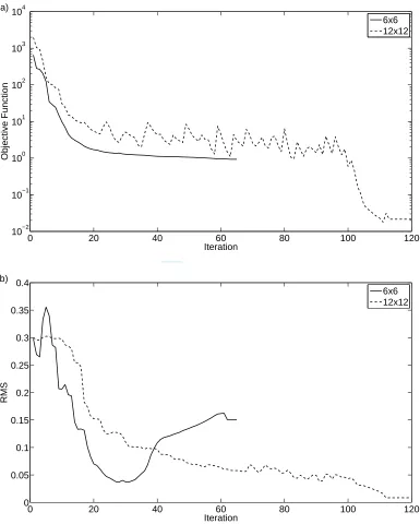
Figures 3(a) and 3(b) display the value of the objective function (18) minimized by the MATLAB routine ‘fmincon’ and the RMS value (26), as functions of the number of iterations, respectively. Results shown were obtained taking MFS parametersM =N = 6 and 12, withK= 2M−1 = 11 and 23, respectively. In these cases, the objective functional (18) containsN(5M+ 1) = 186 and 732 conditions, respectively. Results are summarised in Table 1.

For Peer Review

0 20 40 60 80 100 120

10−2 10−1 100 101 102 103 104

Iteration

Objective Function

6x6 12x12 a)

0 20 40 60 80 100 120

0 0.05 0.1 0.15 0.2 0.25 0.3 0.35 0.4

Iteration

RMS

6x6 12x12 b)

Figure 3: a) The objective function (18) and b) the RMS values (26) for MFS parametersM =N = 6 and 12,K= 11 and 23, respectively.

From Figure 3, when considering the case M =N = 6, it can be seen that even though the objective function continues to decrease, the RMS value begins to diverge at a given point. In order to see if this holds true when we increase the values of the MFS parameters, analysis of the problem with parameters

M =N = 12, K = 2M −1 = 23 is carried out. The numerical results for the objective function (18) and the RMS values (26) for these new MFS parameters are also shown in Figure 3. By comparing the results presented in Figure 3, it can be seen that the RMS value no longer increases as the MFS parameter values increase. In Figure 3(a), for MFS parameters M =N = 12, after 118 iterations the objective function (18) appears to reach a stationary value, this can also be confirmed by studying the RMS values in Figure 3(b).

For Peer Review

In order to demonstrate the performance of the minimisation process, a graphical representation of the internal boundary at various iteration numbers, for MFS parametersM =N = 12 is shown in Figure 4. From this figure it can be seen that a convergent and stable reconstruction of the moving inclusion is realised after 118 iterations. This corresponds to the objective function becoming constant.

Figure 4: Plots of the inclusion at iterations: a) 42, b) 90, and c) 118 (final), when trying to locate a circular inclusion of radius 0.5. d) Shows the initial guess and the final solution.

The solver was run for a variety of MFS parameters. A parameter set of M =N = 12, K = 23 was deemed sufficiently large for the purposes of achieving an accurate result when balanced with the high computational time required for larger MFS parameter values. It can be clearly seen from the results presented in Table 1 that as the parameter size increases, the overall accuracy of the estimated solution increases. One can also deduce from Table 1, that larger parameter sets require more iterations, in order to reach a stable solution, the time for each iteration also increases with increasing parameter size. 6

For Peer Review

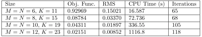
Size Obj. Func. RMS CPU Time (s) Iterations

M =N= 6, K= 11 0.92969 0.15021 16.587 65

M =N= 8, K= 15 0.08784 0.03370 72.736 68

M =N= 10,K= 19 0.04311 0.01897 336.55 105

M =N= 12,K= 23 0.02151 0.00852 1116.8 118

Table 1: Numerical results for the objective function (18), the RMS (26), the CPU time and the number of iterations required for convergence, obtained with various MFS parameter sizes.

4.1.2 Introduction of Noise to the Boundary Flux Data

In reality, the heat flux values (4) on the boundary ∂Ω would be measured using experimental tech-niques. Due to this, a numerical noise factor is numerically simulated to mimic the inherent errors in the experimental data that would be used. Noisy data was achieved by using the MATLAB function

normrand(0, σ), which generates a random number from a given normal distribution space, namely,

gη(xj_i, tj) =g(xji, tj) +ǫi,j= 2 +ǫi,j, i= 1, N , j = 0, M , (27)

whereǫi,j are normal random variables with mean 0 and standard deviationσ=max|g(xji, tj)|p, wherep

represents the percentage of noise.

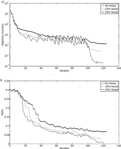
Figures 5(a) and 5(b) display the objective function (18) and the RMS value (26), as functions of the number of iterations, respectively, for both p= 10% and 25% noise added in the flux data (25), as in (27). From these figures it can be observed that introducing noise decreases the accuracy and stability of the solution. In order to further confirm this statement, a graphical representation of the solution is given in Figure 6. Results are summarised in Table 2.

For Peer Review

0 20 40 60 80 100 120 140

10−2 10−1 100 101 102 103 104

Iteration

Objective Function

No Noise 10% Noise 25% Noise a)

0 20 40 60 80 100 120 140

0 0.05 0.1 0.15 0.2 0.25 0.3 0.35

Iteration

RMS

No Noise 10% Noise 25% Noise b)

Figure 5: a) The objective function (18), and b) the RMS values (26) for MFS parametersM =N = 12, K = 23, forp= 0, 10% and 25% noise.

For Peer Review

Figure 6: Final plot of the inclusion after the final 107 iterations. M =N= 12,K= 23, for a)p= 10%, and b)p= 25% noise.

From Figure 5 it can be observed, as expected, that the numerical results become less accurate and stable as the amount of noise increases from for p= 10% to 25% noise. However, the numerical solution for

p= 25% noise is still in reasonable agreement with the exact solution bearing in mind the rather large amount of noise with which the input flux data has been contaminated. The relatively high robustness with these large amounts of noise is potentially related to the simple geometry of the inclusion being reconstructed. It is not anticipated that this would be the case with more challenging geometries, as investigated in later examples.

By taking a plot of the final solution at the final time, t = T = 1, the effects of increasing the noise can be seen from Figure 7 and Table 2. It can be observed that as the amount of noise decreases the numerical solution approximates better the exact solution.

For Peer Review

Figure 7: Reconstructed inclusion at t=T = 1, withM =N = 12,K= 23, for various levels of noise.

Overall, the numerical results obtained for Example 1 demonstrate that the MFS provides a powerful method for solving inverse geometric problems concerned with the reconstruction of simple smooth internal boundaries, such as a circle. The method provides a simpler alternative from using discretisation methods such as the BEM or the FEM, which can often be complicated when meshing moving geometries. It has been shown that high levels of accuracy and resolution can be obtained for a simple geometry such as a circular inclusion, however, the addition of noise in the input data can cause a decrease in the resolution and stability.

Noise (%) Obj. Func. RMS Iterations 0 0.02151 0.00852 118 5 0.10689 0.02030 109 10 0.27019 0.03119 118 25 1.40198 0.06796 122

Table 2: Numerical results for the objective function (18), the RMS (26) and the number of iterations required for convergence, obtained withM =N = 12,K= 23 and various levels of noise.

4.2

Example 2

Here we attempt to locate a bean shaped stationary star-shaped inclusionD parametrised by

r(θ) =0.55 + 0.4cos(θ) + 0.15sin(2θ)

1 + 0.7cos(θ) , (28) 6

For Peer Review

within the domain Ω =B(0,1). This is a typical validation shape when considering inverse geometric research. The initial and boundary conditions (2), (3) and (5) are given by

u(x,0) =u0(x) = 0, x∈Ω\D(0), (29)

u(x, t) =f(x, t) =xt, (x, t)∈∂Ω×[0, T], (30)

u(x, t) =h(x, t) = 0, (x, t)∈∂D(t)×[0, T], (31) wherex= (x, y).

In a first instance, we assume that the inclusion does not move in time, and that this is knowna priori. Note that in the previous example the source and collocation points were placed in relation to the current location of the inclusion D(t), namely the polar radius r(θ, t) was dependent on both space and time, however as we are now fixing the inclusion throughout time, this parametrisation ofD(t), as a stationary defect D, can indeed be simplified. Due to this simplification the location of source and collocation points need to be modified, as described below.

Equation (12) can now be expressed as,

yjm+N =

1

2(rjcos(θj), rjsin(θj)), j = 1, N , m= 1,2M , (32) where the radii r(θj) =: rj ∈ (0,1) constitute a radial parameterisation of the stationary star-shaped

domainD whose boundary at any timet∈(−T, T) is approximated by,

∂D=

r(θj) cos(θj), r(θj) sin(θj)|j= 1, N . (33)

By comparing this with equations (9) and (13), one can now observe that the radial parametrisation is no longer dependent on time, but only on its position in space. Modifications to the position of the inclusion dependent collocation points will now be stated.

Equations (15) and (16) now become

(xj_i, τj) = (ricos(θi), risin(θi), τj), i= 1, N , j= 0, M , (34)

xi,j=

rj+

(1−rj)i

K

cos(θj),

rj+

(1−rj)i

K

sin(θj)

, i= 1,(K−1), j = 1, N , (35)

The final problem entails to 4M N +N =N(4M + 1) unknowns represented by the 4M N coefficients

c= (cm j )

m=1,2M

j=1,2N in the MFS expression (7), and theN radiir= (rj)j=1,N.

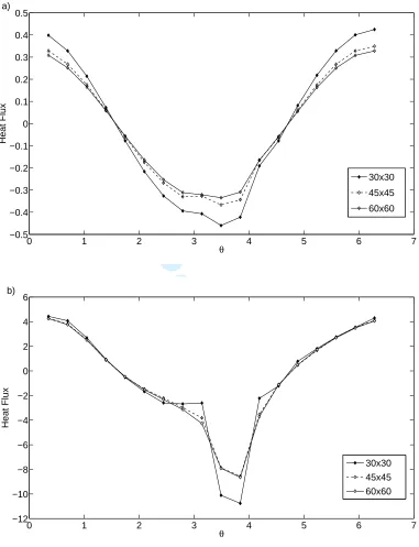
As described previously, the inverse problem here is a difficult non-linear ill-posed problem, and therefore it is necessary that extra information is supplied in order to satisfy the increased number of unknowns in order to reconstruct the boundary, ∂D(t), within the domain Ω. This information is in the form of the heat flux (4) on∂Ω. Since for the irregular bean shape (28) an analytical solution for the direct problem (1), (29)-(31) is not available, the forward problem is solved numerically using the MFS and the flux is generated for the required boundary collocation points on∂Ω. Figures 8 shows the heat flux values (4) at timest∈ {₁₈1,1}, respectively, obtained by solving the direct problem (1), (29)-(31), with various MFS parameter sizes M =N ∈ {30,45,60} and the regularisation parameterλ= 10−7_{. It can be deduced}

from Figure 8 that the numerical solutions did not change significantly when the MFS parameter sizes were in excess ofM =N= 60.

For Peer Review

0 1 2 3 4 5 6 7

−0.5 −0.4 −0.3 −0.2 −0.1 0 0.1 0.2 0.3 0.4 0.5

θ

Heat Flux

30x30

45x45

60x60 a)

0 1 2 3 4 5 6 7

−12 −10 −8 −6 −4 −2 0 2 4 6

θ

Heat Flux

30x30 45x45 60x60 b)

Figure 8: The heat flux values (4) across∂Ω at times a)t= 1

18, and b)t= 1, for various MFS parameters

sizes.

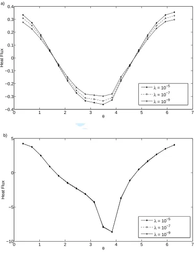
Next, the heat flux values (4) at times t ∈ {₁₈1,1}, obtained by solving the forward problem with the MFS parameter size M =N = 60 are plotted in Figure 9, for various regularisation parameters. The fluxes are output at 18 points across the boundary∂Ω which will be used as data for the inverse problem of Example 2. This way, the inverse problem will be run with the MFS parameter sizeM =N = 18. 6

For Peer Review

0 1 2 3 4 5 6 7

−0.4 −0.3 −0.2 −0.1 0 0.1 0.2 0.3 0.4

θ

Heat Flux

λ = 10−5

λ = 10−7

λ = 10−9 a)

0 1 2 3 4 5 6 7

−10 −5 0 5

θ

Heat Flux

λ = 10−5

λ = 10−7

λ = 10−9 b)

Figure 9: The flux values (4) across ∂Ω at times a) t = 1

18, and b) t = 1, for various regularisation

parameters.

When selecting a suitable regularisation parameter in equation (21) for solving the forward problem, a compromise value is taken, which should be large enough to remove the effects of ill-conditioning of the MFS system of equations, and small enough to have minimal effect on the accuracy of the solution. From Figure 9(a), whenλ= 10−9 _{the ill-conditioning of the system is still visible, however the solution}

appears to to be stable forλ= 10−7_{. As such this value shall be used when solving the forward problem}

for the MFS parameter sizeM =N = 60. 6

For Peer Review

4.2.1 Results

Analysis of the results for Example 2 follow a similar format to that of Example 1. Results for both the objective function (18) and the RMS value

RMS =

s

PN

j=1 rj−rj∗

2

N , (36)

where

r∗

j =r∗(θj) =

0.55 + 0.4cos(θj) + 0.15sin(2θj)

1 + 0.7cos(θj)

, θj =

2πj

N , j= 1, N . (37)

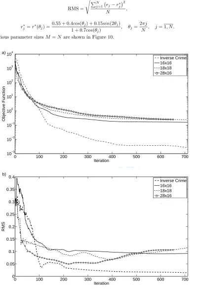
for various parameter sizesM =N are shown in Figure 10.

0 100 200 300 400 500 600 700

10−3 10−2 10−1 100 101 102 103 104

Iteration

Objective Function

Inverse Crime 16x16 18x18 28x16 data5 a)

0 100 200 300 400 500 600 700

0 0.05 0.1 0.15 0.2 0.25 0.3 0.35 0.4

RMS

Inverse Crime 16x16 18x18 28x16 data5 b)

For Peer Review

From Figure 10 it can be seen that as the MFS parameter size increases, the accuracy of the solution also increases. To further confirm the functionality of the optimisation process, an ’inverse crime’ is also committed (i.e. the heat flux data is generated using the same forward mesh size in the inverse problem). From these results it can be observed that the error is very small in relation to the other parameter sizes, hence providing further confirmation that the solver is functioning correctly.

Unlike the majority of previous works where the MFS is used to solve steady state inverse problems, the time-dependent case produces a much larger system of unknowns and as such, the objective function is more costly to evaluate. Due to this, parameter sizes typically have to be smaller than those used in aforementioned works otherwise, the computational time required to solve becomes unfeasibly large. A parameter size ofM = 26,N = 16 has been found to be the largest parameter size when drawing a com-promise between accuracy and computational expense. A two-dimensional plot of the results obtained is displayed in Figure 11. As the solution remains stationary in time, it is unnecessary to provide a full space-time plot of the inclusion.

As one can observe from Figures 10(a) and 11, as the parameter size increases, the accuracy of the numerical solution also increases. In order to further highlight this, a plot of the absolute errors squared versus the polar angleθ, is given in Figure 12.

0.2 0.4

0.6 0.8

1

30

210

60

240

90

270 120

300 150

330 180

Actual 28x16 18x18 16x16

Figure 11: Plot of the inclusion for various MFS parameter sizes. 6

For Peer Review

0 1 2 3 4 5 6 7

0 0.005 0.01 0.015 0.02 0.025 0.03 0.035 0.04 0.045

θ

Error

2

16x16 18x18 28x16 Inverse Crime

Figure 12: The absolute error squared versusθ for various MFS parameter sizes.

From examining Figure 12 it can be observed that as the mesh size increases the accuracy generally increases. One can also observe that the level of error from performing the inverse crime is very small, providing reassurance that the computational code and methodology are correct.

As explained in section 4.1.2, it is deemed necessary to consider noise in order to simulate data similar to that obtained from physical means of measurements. Previous works using the MFS for steady state problems have shown it beneficial to use Tikhonov regularisation (see section 3.3) for solving inverse problems with noisy data.

Trials were carried out using the generated noisy data for a variety of regularisation parametersλ. The residual (18) and RMS values (36) for these trials are shown in Figure 13. Note that the residual takes the form of (18), where (20) is the regularised objective function being minimised. The residual (18) was plotted in Figure 13(a) rather than the usual objective function (20), as this is necessary in order to use a discrepancy principle, the details of which are explained in later text.

For Peer Review

0 100 200 300 400 500 600 700

10−1 100 101 102 103 104

Iteration

Residual

λ = 0

λ = 10−1

λ = 10−2

λ = 10−3

ε2

a)

0 100 200 300 400 500 600 700

0.05 0.1 0.15 0.2 0.25 0.3 0.35 0.4

Iteration

RMS

λ = 0

λ = 10−1

λ = 10−2

λ = 10−3 b)

Figure 13: a) The residual (18), and b) the RMS values (36) for various regularisation parameters when the heat flux data (4) is contaminated with 1% noise.

In physical applications where the input data is likely to be contaminated with noise it is necessary to have a stopping criterion for the iterative procedure in order to prevent the solution becoming unstable. For trials were no regularisation was imposed, i.e. the objective function (18) is minimised, the iteration was stopped at the iteration number for which the residual (18) attains approximately the noise level,

ǫ2=

N

X

i=1

M

X

j=0

(gη(xj_i, tj)−g(xji, tj))2. (38)

This is known as the discrepancy principle and it is graphically illustrated in Figure 13(a) where the value ofǫ2_{is shown as the horizontal line. In cases where regularisation was imposed, a fixed number of}

For Peer Review

were plotted in Figure 14 for various values of λ, and λwas chosen based on which residual after 300 iterations was closest to the value of ǫ2_{(= 3.9 for 1% noise in Example 2). This is also termed as the}

discrepancy principle. Figure 14 shows that this value is betweenλ= 10−3 _{and 10}−2_.

10−6 10−5 10−4 10−3 10−2 10−1

0 2 4 6 8 10 12 14 16 18

λ

Residual

ε2

Figure 14: Residuals after 300 iterations for various values ofλ.

RMS values for trials with 1% noise and Tikhonov regularisation in conjunction with the two discrepancy principles described above are shown in Table 3. The corresponding numerical reconstructions of the inclusion are shown in Figure 15.

Noise (%) RMS Regularisation (λ) Iteration@Final Result

0 0.043 0 220

1 0.069 0 131

1 0.0616 0.001 300 1 0.1151 0.01 300

Table 3: Numerical results for the RMS (36) obtained withM = 28,N = 16 andK= 55. 6

For Peer Review

0.4 0.6

0.8 1

30

210

60

240

90

270 120

300 150

330

180 0

0% Noise (Optimal Solution) 1% Noise, λ = 0, 131 iterations (Discrepancy principle) Target Solution

a)

0.2 0.4

0.6 0.8

1

30

210

60

240

90

270 120

300 150

330

180 0

Target

1% Noise, λ = 0.01, 300 iterations 1% Noise, λ = 0.001, 300 iterations

b)

Figure 15: a) Plot of the inclusion for 0 and 1% noise. The iteration process is stopped according to the first discrepancy principle. b) Plot of the inclusion for 1% noise. The regularisation parameter is chosen according to the second discrepancy principle.

Figure 15(a) demonstrates that the method proposed is stable with respect to small amounts of noise in the input data. Results presented within this figure show that the formation shape, with no regularisation 6

For Peer Review

and stopped using the first discrepancy principle (based on Figure 15(a)) is very close to the optimal solution shown when using 0% noise, i.e. exact data. Both 0 and 1% input data generate good likeness to the target solution, with the largest error occurring near the cusp region. The numerical results presented in Figure 15(b), obtained using the regularisation parameterλchosen according to the second discrepancy principle (based on Figure 14), do not show much improvement over the results presented in Figure 15(a).

4.3

Example 3

As in Example 2, we attempt to locate a stationary star-shaped inclusionDparametrised by

r(θ) =0.55 + 0.4cos(θ) + 0.15sin(2θ)

1 + 0.7cos(θ) , (39) within the domain Ω =B(0,1). However, this time we impose no assumption that the boundary∂D(t) is stationary throughout timet∈(0, T = 1). The initial and boundary conditions are given by equations (29)-(31). In order to ensure a unique solution it is imposed that D(0) is known, see Kawakami and Tsuchiya (2010), and therefore we solve for a non-linear system of 5M N unknowns.

4.3.1 Results

Analysis of the results for Example 3 follow a similar format to that of the previous examples. The RMS now takes the form,

RMS =

v u u t

PN

j=1

PM

m=0 rmj −r∗j

2

N(M+ 1) , (40)

wherer∗

j are given by equation (37). Initial results presented correspond to MFS parameters of varying

sizes. 6

For Peer Review

0 100 200 300 400 500 600

10−1 100 101 102 103 104

Iteration

Objective Function

16x16 18x18 28x16 a)

0 100 200 300 400 500 600

0.1 0.15 0.2 0.25 0.3 0.35 0.4 0.45

Iteration

RMS

16x16 18x18 28x16 b)

Figure 16: a) The objective function (18), and b) the RMS values (40) for various MFS parameter sizes.

Figure 16(a) shows the objective function decreasing, and the solver attempting to locate the interior formation. Unlike Example 2, there only appears to be a small correlation between increasing the mesh size and RMS values. The minimum achievable RMS value, using the MFS parameters presented here, in Figure 16(b), appears to be around 0.1. In order to further understand the reasoning for these relatively low accuracies, Figure 17 plots the errors in both time and space. From Figure 17 it can be observed that the errors predominate close to the initial time (t= 0) and also close to the concave region of the cusp, but accuracy in other regions is generally of a good standard. In order to further confirm that this statement applies for all tested cases, Figure 18 shows the average absolute error for each given time. From this figure it can be seen that for all MFS parameters attempted within Example 3, the error is largest at times close tot= 0, and slowly decreases as time increases.

For Peer Review

0.1 0.2

0.3 0.4

0.5 0.6

0.7 0.8

0.9

1 0

1 2

3 4

5 6 0

0.1 0.2 0.3 0.4

θ

t

Absolute Error

0 0.05 0.1 0.15 0.2 0.25 0.3

Figure 17: The absolute error between the target and obtained solution for M =N = 18 at iteration 171.

0 0.1 0.2 0.3 0.4 0.5 0.6 0.7 0.8 0.9 1

0 0.02 0.04 0.06 0.08 0.1 0.12 0.14 0.16

Time

Mean absolute error at given time

28x16 18x18 16x16

Figure 18: The mean absolute error between the target and obtained solution over time for a variety of MFS parameters at optimal stopping iterations.

Finally, Figure 19 shows a full plot for the inclusion, as a function ofxand . From this figure it can be 6

For Peer Review

Figure 19: Plot of the inclusion forM =N = 18 after 171 iterations.

Despite the aforementioned problems when using the method proposed for Example 3, excluding the initial solution times, where noticeable errors were observed, the solver’s ability to reconstruct the internal structure appears to function well. An example of such a solution at the final timet=T = 1 is shown in Figure 20.

For Peer Review

0.4 0.6

0.8 1

30

210

60

240

90

270 120

300 150

330

180 0

16x16

18x18

28x16

Target

Figure 20: Plot of the inclusion at the final timet=T= 1, for various MFS parameter sizes.

It was considered unnecessary to illustrate trials with artificial noise imposed on the input data, though we report that the same stable numerical solutions, as in Example 2, are expected. Instead of this, we consider in the next example the case of a fully moving internal target.

4.4

Example 4

In this final example, we attempt to reconstruct an internal moving boundary star-shaped inclusionD(t) parametrised by

r(t) = 0.9− t

2, t∈[0, T], (41) within the domain Ω =B(0,1). The initial and boundary conditions (2) and (5) are given by (29) and (31), and the Dirichlet boundary condition is taken as,

u(x, t) =f(x, t) =t, (x, t)∈∂Ω×[0, T]. (42) As in Example 3, in order to ensure a unique solution to the inverse problem, we assume that the circular shaper(0) = 0.9 of the inclusionD(0) at the initial timet= 0 is known.

In this example we have chosen to remove the added complexity of the bean shaped formation, to see if the method has the ability to reconstruct a simple moving circular formation, as parametrised by equation (41). Due to the simplicity of the shape, MFS parameter sizes similar to those in Example 1 were used. Input data was obtained by solving the forward problem, as described in Example 2, specific parameters and resulting figures for which are omitted here.

For Peer Review

0 50 100 150 200 250 300 350

10−6 10−4 10−2 100 102 104

Iteration

Objective Function

8x8 10x10 12x12 a)

0 50 100 150 200 250 300 350

0 0.05 0.1 0.15 0.2 0.25 0.3 0.35 0.4

Iteration

RMS

8x8 10x10 12x12 b)

Figure 21: a) The objective function (18), and b) the RMS values (40) for various MFS parameters.

From Figure 21, numerical results with lower MFS parameter sizes appear to produce different results to what the previous examples would imply. Generally, the smaller parameter sizes produce more stable results. In order to look for reasoning behind this, Figure 22 shows the absolute error across the interior reconstruction for the MFS parameter sizes M = N = 8 and 12. From Figure 22 it can be seen that as the MFS parameter size increases, the effects of the ill-conditioning start to become apparent. These effects appear to be dominant close to t= 0, as in Example 3. The small MFS parameter sizes appear to reduce this error, however the errors remain larger at times away fromt= 0 than those for the larger MFS parameter sizes. In order to illustrate more clearly this point, Figure 23 shows the mean absolute errors, between the target and obtained solution at the various times.

For Peer Review

Figure 22: The absolute error between the target and obtained solution for a) M = N = 8, and b)

M =N = 12 at optimal stopping iterations.

0 0.1 0.2 0.3 0.4 0.5 0.6 0.7 0.8 0.9 1

0 0.05 0.1 0.15 0.2 0.25 0.3 0.35 t

Mean absolute error at given time

12x12 10x10 8x8

Figure 23: The mean absolute error between the target and obtained solution over time for a variety of MFS parameters at optimal stopping iterations.

Finally in order to further visualise and interpret the above numerical results, Figure 24 shows the full space-time solution for parametersM =N = 8 and 12.

For Peer Review

Figure 24: The moving inclusion for: a) M = N = 8, and b) M = N = 12 at the optimal stopping iterations.

5

Conclusions

This paper has used a variety of examples to test both the accuracy and stability of the proposed regularised MFS for solving a non-linear geometric inverse problem, namely the two-dimensional time dependent heat equation to locate an unknown internal boundary.

Example 1 demonstrates that simple boundaries can be located to high degrees of accuracy and sta-bility.

Example 2 demonstrates, assuming the boundary remains fixed in time, that complex ’bean-shaped’ boundaries can be located with a reasonable high level of accuracy and stability.

Example 3 no longer assumes that the boundary was fixed in time, removing this constraint severely impaired accuracy of the inclusion reconstruction, increasing mesh size had little effect rectifying this. Despite this, inclusions were approximated to a reasonable level of accuracy, with the largest errors ap-pearing at times close tot= 0.

Example 4 shows that the method presented here can successfully locate simple moving boundaries, however like Example 3, large errors are present at times close tot= 0. It was shown that these can be partially removed by using smaller MFS parameter sizes, however this was at the expense of both the accuracy when considering times away from the initial point and of the overall formation resolution.

Extension of the method to three-dimensions is a viable option and will likely provide useful to the practical application discussed in the introduction.

Acknowledgments

The authors would like to thank both the ESPRC and National Nuclear Laboratory for continual funding and support.

References

1. D. Borman, D. B. Ingham, B. T. Johansson and D. Lesnic (2009) The method of fundamental solu-tions for detection of cavities in EIT,Journal of Integral Equations and Applications, 21, 383-406. 6

For Peer Review

2. K. Bryan and L.F. Caudill, Jr (1998) Stability and reconstruction for an inverse problem for the heat equation,Inverse Problems,14, 1429-1453.

3. R. H. Byrd, J. C. Gilbert and J. Nocedal (2000) A trust region method based on interior point techniques for nonlinear programming,Mathematical Programming,89, 149-185.

4. K. Chaji and M. El Bagdouri (2008) Identification of an internal material boundary,Inverse Problems in Science and Engineering, 16, 511-522.

5. K. Chaji, M. El Bagdouri and R. Channa (2008) A 2D domain boundary estimation, Journal of Physics: Conference Series,135, 012029.

6. S. Chantasiriwan, B.T. Johansson and D. Lesnic (2009) The method of fundamental solutions for free surface Stefan problems,Engineering Analysis with Boundary Elements,33, 529-538.

7. R. Chapko, R. Kress and J.R. Yoon (1998) On the numerical solution of an inverse boundary value problem for the heat equation,Inverse Problems,14, 853.

8. R. Chapko, R. Kress and J.R. Yoon (1999) An inverse boundary value problem for the heat equation: the Neumann condition,Inverse Problems,15, 1033.

9. C.S. Chen, H. A. Cho, M.A. Golberg (2006) Some comments on the ill-conditioning of the method of fundamental solutions,Engineering Analysis with Boundary Elements, 30, 405-410.

10. Y.C. Hon and M. Li (2008) A computational method for inverse free boundary determination prob-lem, International Journal for Numerical Methods in Engineering,73, 1291-1309.

11. M. Ikehata and M. Kawashita (2010) On the reconstruction of inclusions in a heat conductive body from dynamical boundary data over a finite time interval,Inverse Problems,26, 095004 (15pp).

12. B.T. Johansson, D. Lesnic and T. Reeve (2011) A method of fundamental solutions for two-dimensional heat conduction,International Journal of Computer Mathematics,88, 1697-1713.

13. A. Karageorghis and D. Lesnic (2009) Dectection of cavities using the method of fundamental solu-tions,Inverse Problems in Science and Engineering,17, 803-820.

14. A. Karageorghis, and D. Lesnic (2011) Application of the MFS to inverse scattering problems, En-gineering Analysis with Boundary Elements,35, 631-638.

15. H. Kawakami, Y. Moriyama and M. Tsuchiya (2007) An estimation problem for the shape of a domain varying with time via parabolic equations,Inverse Problems,23, 755-783.

16. H. Kawakami and M. Tsuchiya (2010) Uniqueness in shape identification of a time-varying domain and related parabolic equations on non-cylindrical domains,Inverse Problems, 26, 125007 (34pp).

17. S. Vessella (2008) Quantitative estimates of unique continuation for parabolic equations, determina-tion of unknown time-varying boundaires and optimal stability estimates, Inverse Problems,24, 023001 (81pp).