Skew-varicose instability in two-dimensional generalized Swift-Hohenberg equations

promoting access to White Rose research papers

White Rose Research Online

[email protected]

Universities of Leeds, Sheffield and York

http://eprints.whiterose.ac.uk/

This is an author produced version of a paper published in

Physical Review E

White Rose Research Online URL for this paper:

http://eprints.whiterose.ac.uk/43322/

Paper:

Weliwita, JA, Rucklidge, AM and Tobias, SM (2011)

Skew-varicose instability in

two-dimensional generalized Swift-Hohenberg equations.

Physical Review E, 84

(3).

arXiv:1107.4917v2 [math.DS] 26 Jul 2011

SKEW-VARICOSE INSTABILITY IN TWO DIMENSIONAL

GENERALIZED SWIFT–HOHENBERG EQUATIONS

J. A. Weliwita,∗ _{A. M. Rucklidge,}† _{and S.M. Tobias}‡ Department of Applied Mathematics,

University of Leeds, Leeds LS2 9JT, UK. (Dated: August 12, 2011)

We apply analytical and numerical methods to study the linear stability of stripe patterns in two generalizations of the two-dimensional Swift–Hohenberg equation that include coupling to a mean flow. A projection operator is included in our models to allow exact stripe solutions. In the generalized models, stripes become unstable to the skew-varicose, oscillatory skew-varicose and cross-roll instabilities, in addition to the usual Eckhaus and zigzag instabilities. We analytically derive stability boundaries for the skew-varicose instability in various cases, including several asymptotic limits. We also use numerical techniques to determine eigenvalues and hence stability boundaries of other instabilities. We extend our analysis to both stress-free and no-slip boundary conditions and we note a cross over from the behaviour characteristic of no-slip to that of stress-free boundaries as the coupling to the mean flow increases or as the Prandtl number decreases.

Close to the critical value of the bifurcation parameter, the skew varicose instability has the same curvature as the Eckhaus instability provided the coupling to the mean flow is greater than a critical value. The region of stable stripes is completely eliminated by the cross-roll instability for large coupling to the mean flow.

I. INTRODUCTION

Spiral defect chaos (SDC) was discovered in low-viscosity convection nearly 20 years ago [1], and yet much of the detail of its origin remain unexplained. The Swift–Hohenberg equation (SHE), originally proposed as a model equation for fluctuations near the onset of con-vection [2], has yielded considerable insight into the ques-tion of wavenumber selecques-tion in pattern formaques-tion [3]. However the SHE has a major drawback as a model of low-viscosity convection: mean flows are excluded. The importance of the large scale mean flow on the stability of convection rolls was first investigated by Siggia and Zip-pelius [4]. Mean flows are known to play an important role in the dynamics of spiral defect chaos [5], and so two related generalizations of the SHE have been developed to include the effects of mean flows [6, 7].

SDC was found numerically in solutions of one of these generalized Swift–Hohenberg equations [7, 8] and of the Boussinesq equations for convection [5, 9–12]. The gen-eralized SHE can reproduce some qualitative features of spiral defect chaos, at least as transients, though direct comparison between the model and convection appears not to be appropriate [13].

Including mean flows in these models allows an inter-esting long-wavelength instability, the skew-varicose in-stability (SVI) [14] whose spatial dependence is neither entirely longitudinal nor transverse to the local pattern wavevector. The SVI resembles the Eckhaus instability but the most unstable modes are those at an angle to

∗_{[email protected]}

†_{http://www.maths.leeds.ac.uk/˜alastair/} ‡_{http://www.maths.leeds.ac.uk/˜smt/}

the original roll axes. In the SVI, rolls bend and become irregular in order to decrease their effective wavenum-ber, and often dislocation pairs will form [3]. Indeed, chaotic spiral patterns have been observed during the transition from the conducting state to rolls. Mean flows are also crucial to the formation of SDC: Chiamet al._[5]

showed that spiral defect chaos collapses to a stationary pattern when the mean flow is quenched. The onset of SDC and defect chaos has therefore been tentatively as-sociated with the occurrence of the SVI [12, 15, 16]. It is this connection that motivates this detailed investigation into the SVI.

The classical problem of linear stability of convection rolls with stress-free horizontal boundaries near the on-set of convection has been studied by a number of au-thors [17–20], while the linear stability of convection with no-slip boundaries [21] is much less well understood. An additional problem that occurs in the analysis of the SVI is that there is no consistent relative scaling of lengths parallel and perpendicular to the roll axes, owing to the singular nature of the slow length scale expansion of the stability problem, as detailed below.

SVI boundary for stress-free and no-slip convection from the Boussinesq equations for convection. However, the perturbation terms that they included in their calcula-tions do not adequately capture the mechanism of the SVI in all circumstances [24]. Milke [25] carried out a more comprehensive study of stability of rolls by means of a Lyapunov–Schmidt reduction. He recovered domains in Rayleigh, Prandtl and wave number space where con-vection rolls are unstable, the so-called Busse balloon.

In this paper, we revisit the two generalized SH models that include a coupling to the mean flow [6, 7, 26, 27], and analyse in detail how the skew-varicose instability depends on the parameters in the models.

Although the model equations of interest have been well studied, a complete analysis of the SVI in the models is not available. One difficulty in the analysis comes from the contribution of terms proportional tok2_l2_/(k2_+l2_),

where (k, l) is the small wavevector of the perturbations associated with the SVI. Terms like this are responsible for the absence of a consistent asymptotic scaling in the limit of small amplitude and small k and l [28]. This difficulty is resolved in this paper.

The remaining part of this paper is organized as fol-lows: in section (II), we present the two generalizations of the Swift–Hohenberg equation, both of which incorpo-rate the effect of a mean flow. We discuss two operators:

Pαis a projection operator included in the model to allow

exact stripe solutions, andFγ is a filtering operator that

suppresses the cross-roll instability. _Fγ is present in an

original formulation of the models [26];_Pαwas suggested

by Ian Melbourne [29]. In section (III), we present a de-tailed analysis of the linear stability of the stripe solution, showing how the SVI can be located analytically. We ex-plore the importance of the mean flow in long-wavelength instabilities. The structure of the maximum eigenvalue for instability for smallkandl is also presented.

In section (IV), we analyze the zigzag and Eckhaus long-wavelength instabilities. Section (V) describes the interesting skew-varicose instability. We also consider various asymptotic limits.

The work is extended in section (VI) to the stress-free boundary condition case, for which there are skew-varicose and oscillatory skew-skew-varicose instabilities. Sec-tion (VII) covers short-wavelength instabilities (the cross-roll instability) for stress-free and no-slip bound-ary conditions. Some numerical illustrations of stability boundaries with growth rates of perturbations are illus-trated in section (VIII), where we also discuss some cu-rious behavior of the growth rates of perturbations. Fi-nally, in section (IX), we show how the region of stable stripes is affected by the coupling to the mean flow and how it can be completely eliminated if the coupling is strong enough, in the stress-free case. We conclude in section (X).

II. PROBLEM DEFINITION

In this section, we set out the two models we will inves-tigate, and discuss basic properties of the models. Both models are generalizations of the two-dimensional Swift– Hohenberg equation, where a real fieldψ(x, y, t), repre-senting the amplitude of convection, couples to a mean flow given by a stream functionζ(x, y, t) and its vertical vorticityω(x, y, t) =_−∇2_ζ.

A. Description of Models

The standard Swift–Hohenberg equation [2] is

∂ψ

∂t =

µ−(1 +∇2)2ψ−ψ3, (1)

whereψ(x, y, t) represents the pattern-forming field, and

µ is the driving parameter (in convection,µ represents the temperature difference between the top and the bot-tom layer), taking the value zero at the onset of pattern formation. Both models introduce a (U_{· ∇)ψ term to} the right-hand side of (1), whereU_{(x, y, t) is a mean flow} calculated from the stream functionζ(x, y, t):

U₌

∂ζ

∂y,−

∂ζ ∂x

.

The mean flow has vertical vorticityω(x, y, t) = −∇2_ζ.

The way that vorticity is generated by nonlinear forcing fromψdiffers in the two models.

In the first model [7], the vertical vorticity ω(x, y, t) has its own independent dynamics:

∂ψ

∂t + (U· ∇)ψ=

µ₋(1 +_∇2₎2_ψ

− Pα ψ3

,

(2)

∂

∂t−P r(∇

2 −c2)

ω=−gmFγ

∇(∇2ψ)× ∇ψ·bz_, (3)

whereP r, c andgm are parameters. The Prandtl

num-berP r (the ratio between kinematic viscosity and ther-mal diffusivity) is effectively a viscosity parameter for the mean flow, which plays a much greater role in low Prandtl number convection. Indeed, in the limit of largeP r, the vertical vorticity is hardly excited and the dynamics ofψ

becomes purely relaxational [3, 13, 30], reducing model 1 back to the SHE. The coefficient gm is a coupling

pa-rameter that controls the strength of the mean flow ef-fects relative to the ordinary Swift–Hohenberg nonlinear term ₋ψ3_{. The parameter c models the effect of top}

0 1 0

K

σ

-1

µ= 0 -P rc2

FIG. 1. (Color online) Growth rates as functions of wavenum-berK =|K|. Dashed blue curve: σ1 forµ= 0, which peaks

atK=Kcritical= 1. Solid green curve: σ2, which takes the

value−P r c2 _{atK= 0 and decreases asK increases.}

zero in the absence of nonlinear forcing). The operators

Pα andFγ are explained in more detail below.

The second model [6, 26, 27] has the vertical vorticity slaved to the nonlinear driving term:

∂ψ

∂t + (U· ∇)ψ=

µ₋(1 +_∇2)2ψ_{− P}α ψ3

, (4)

ω=₋g_Fγ

∇(_∇2ψ)_{× ∇}ψ_·bz_{, (5)}

so the vertical vorticity responds instantly to the non-linear driving. The coefficientg is a coupling parameter that controls the relative strength of mean flow effects compared to the ordinary nonlinearity.

We use two operators_Pαand Fγ to ease the analysis

and to ensure that the SVI is not pre-empted by other instabilities. They both act as filters in Fourier space; the first is a projection:

Pα(eiK·x) =

eiK·x _if|K|≤α;

0 if|K|>α.

By settingα= 2.5, we allow stripes with a single Fourier mode with wavenumber close to one to be exact solu-tions of the PDEs (2–3) and (4–5) [29]. This is shown in section (II B) below. The second operator, _Fγ, reduces

short-wavelength modulations of the mean flow [26]: in Fourier space, the operator is defined by

Fγ(eiK·x) =e−γ 2

|K|2 eiK·x_.

Throughout this work, we setγ= 2.5. The effect of this filtering on short-wavelength instabilities, particularly the cross-roll instability, is discussed in section (VII).

B. Basic Properties of the Models

For model 1, linearisation yields:

∂ψ

∂t =

µ−(1 +∇2)2ψ and ∂ω

∂t =P r ∇

2

−c2ω;

only the first equation is relevant to model 2. Normal mode solutions to these linear equations are given by

ψ=F1eσ1t+iK·x and ω=F2eσ2t+iK·x, whereσ1 and σ2

are growth rates,K _{is a wavevector, andF1 and F2 are} constants. Substituting these into the linearized equa-tions givesσ1=µ− 1−K2

2

andσ2=−P r K2+c2.

These are shown in Figure 1 for µ = 0, when the trivial solution is marginally stable. The most unstable wavenumber is Kcritical = 1, and for µ > 0, a band of

wavenumbers close toK= 1 is linearly unstable, signal-ing the onset of pattern formation. The vorticityω (in model 1) is always linearly damped, unlessc= 0.

We defineq=K₋Kcriticaland thus the trivial solution

loses stability for anyqatµExistence, where

µExistence= (1−(1 +q)2)2.

Note that asq→0,µExistence →4q2.

In this paper, we are interested in the stability of the nonlinear equilibrium stripe solution of the PDEs. We note that

ψ0=

p

βei(1+q)x_+e−i(1+q)x_{, ω}

0= 0

with β= µ−(1−(1 +q)

2₎2

3 , (6)

is anexact _{solution of both models. This can be shown}

by substituting the expressions for ψ0 and ω0 into the

PDEs:

0 =µpβei(1+q)x+e−i(1+q)x−(1 +∇2)2pβei(1+q)x

+e−i(1+q)x_{− P} α

p

βei(1+q)x_+e−i(1+q)x3

.

The nonlinear term in the vorticity equation is zero. Next, we note that

(1 +_∇2₎2_e±i(1+q)x_{= (1}

−(1 +q)2₎2_e±i(1+q)x

and

P2.5 p

βei(1+q)x+e−i(1+q)x3

= 3βpβ

×ei(1+q)x_+e−i(1+q)x_,

provided thatq is between₋0.167 and 1.5. The conse-quence is that (ψ0, ω0) is an exact solution. In the limit

of smallq, we haveβ = (µ−4q2_{)/3, so stripe solutions}

exist whenµ >4q2_.

The advantage of using the projection_Pα is that it

al-lows this exact stripe solution of the PDEs [29]. The alternative would be to consider the limit of small µ

andβ, but by having an exact solution, which matches the asymptotic result we would obtain without the pro-jection, we do not have to be concerned with the relative sizes of these parameters compared to other small pa-rameters that will be introduced below.

The two models can be related to each other close to onset, regardless of the projection and filtering. By scal-ing µ = _O ǫ2 _{with ǫ}

scale ∂/∂t→ǫ2_{∂/∂t, and assuming that the}

wavenum-bers that are excited in the vorticity variable ω are of order _O(ǫ), the largest term on the left-hand side of the vorticity equation (2) in model 1 is P r c2_{ω. Thus}

model 1 reduces to model 2 in this limit, with the rela-tiong=gm/(P r c2).

III. LINEAR STABILITY OF STRIPES

The linear stability theory for stripes in the SHE is well known [28]: stripes with wavenumber 1 +q exist provided β > 4q2_{, and they are stable with respect to}

the Ekhaus and zigzag instabilities provided β > 12q2

and q > 0. Once mean flows are included, the zigzag

instability needs to be modified at finite Prandtl num-ber by the presence of mean-flow modes with non-zero vertical vorticity [17, 22]. The Eckhaus instability is un-changed. We consider the stability of the stripe solutions with respect to long-wavelength perturbations, deriving three (model 1) or two (model 2) linear ODEs for the perturbation amplitudes, and so determine the parame-ter regions in which the stripe configuration is stable, as well as the boundary of the SVI.

A. Linearisation

We proceed by considering perturbations to the basic stripe solution. We suppose that the vorticity pertur-bation contains wavevectors (k, l) and (₋k,₋l). These interact with the wavevectors (1 +q,0) and (−1−q,0) in the stripe solution to give four new wavevectors, and

so the perturbed solution can be written asψ=ψ0+ψ ′

andω=ω0+ω ′

, withω0= 0 and

ψ′ =A(t)ei(1+q+k,l)·x_+B(t)ei(−1−q+k,l)·x

+ ¯A(t)e−i(1+q+k,l)·x_{+ ¯B(t)e}i(1+q−k,−l)·x_{, (7)} ω′ =C(t)ei(k,l)·x+ ¯C(t)ei(−k,−l)·x. (8)

We can calculate the stream functionζ fromω(x, y, t) =

−∇2_{ζ by inverting the Laplacian, and hence obtain the}

mean flow:

U₌ i

k2_+l2

C(t)ei(k,l)·x_−C¯(t)e−i(k,l)·x_(l,−k).

We substitute the expression above into the two models and linearize (assuming thatA,B andCare small). Ex-amining the coefficients ofei(1+q+k,l)·x_andei(−1−q+k,l)·x

results in linear ODEs forAandB:

˙

A=

µ₋h1₋(1 +q+k)2+l2i2 −6β

A

−3βB+l(1 +q)

√

β

k2_+l2 C, (9)

˙

B=

µ₋h1₋(₋1₋q+k)2+l2i2₋6β

B

−3βA₋l(1 +q)

√

β

k2_+l2 C .(10)

The termk2_+l2_{, which appears in the denominator of}

the governing equations for ˙Aand ˙B, arises from invert-ing the Laplacian when calculatinvert-ingζand henceU_{in the} linearisation of the (U_{· ∇)ψterm. The equation for C} differs between the two models. In model 1, the coeffi-cient ofei(k,l)·x _yields

˙

C=₋P r k2_+l2_+c2_C+

Fγgml(1 +q) p

βh₋(1 +q₋k)2₋l2_{+ (1 +q)}2i_B+h_{(1 +q+k)}2

+l2

−(1 +q)2i_A.

(11) In model 2, with no intrinsic dynamics forω, there is an algebraic relation betweenC,AandB:

C=_Fγgl(1 +q) p

β ((1 +q+k)2+l2₋(1 +q)2)A+ (₋(1 +q₋k)2₋l2+ (1 +q)2)B. (12)

In Fourier space, the effect of the filtering,_Fγ, is to

re-duce the amplitude of a Fourier component; for the func-tionei(k,l)·x_,F

γreduces the amplitude by the

multiplica-tive factore−γ2 (k2

+l2 )_.

Equations (9–11) for model 1 can be succinctly ex-pressed as:

 

˙

A

˙

B

˙

C 

=



 MM12 MM24 −MM33

gmM5 gmM6 M7

 

 AB

C  =J1

 AB

C  .

Equations (9–10) and (12) for model 2 yield:

_˙

A

˙

B

=

M1+gM3M5 M2+gM3M6

M2−gM3M5 M4−gM3M6

A B

=J2

A B

.

Here, we use the abbreviations:

M1=µ−[1−((1 +q+k)2+l2)]2−6β,

M2=−3β,

M3=−l(1 +q) p

M4=µ−[1−((−1−q+k)2+l2)]2−6β,

M5=e−γ

2 (k2

+l2

)_{l(1 +q)}p_{β[2k(1 +q) +k}2_+l2_],

M6=e−γ

2 (k2

+l2

)_{l(1 +q)}p_{β[2k(1 +q)}

−k2₋l2], M7=−P r(k2+l2+c2).

We note that in the limit (k, l)_→(0,0), we have M7 ≈

−P r c2_{, so it is not surprising (looking at the bottom line}

of the 3×3 matrix for model 1) that long-wavelength in-stabilities in model 1 will depend only on the combination

gm/(P r c2).

B. Determinants in the limit of smallk and l

The characteristic polynomials (and hence the eigen-values, traces and determinants) of each of these Jacobian matrices are even inkandl. Bifurcations occur when an eigenvalue crosses through zero. The stripe solution is stable only if all eigenvalues are negative for all (k, l), so we are interested in extreme values of the eigenvalues as functions of k and l. It can be readily checked that a zero extreme value of the eigenvalue corresponds to a zero extreme value of the determinant. Consequently, we use the determinants ofJ1 andJ2 to assist our analysis

of instabilities. The determinant ofJ1,Det(J1), is:

P₁(1)k4_+P(1)

2 k2l2+P (1) 3 l4

+Q(1)₁ k6_{+· · ·+Q}(1) 4 l6

+R₁(1)k8_{+· · ·+R}(1) 5 l8

+S₁(1)k10_{+· · ·+S}(1) 6 l10

−P r(k2_+l2₎6

k2_+l2 ,

where all coefficientsP_i(1) etc. are functions of µ,q,P r, gm, c and the filtering e−γ 2

(k2 +l2

)_{. The determinant of J} 2, Det(J2), is:

P₁(2)k4_+P(2)

2 k2l2+P

(2)

3 l4

+Q(2)₁ k6_+Q(2)

2 k4l2+Q

(2)

3 k2l4+Q

(2)

4 l6

+R(2)₁ k8₊

· · ·+R(2)₅ l8_{+ (k}2_+l2₎5

k2_+l2 ,

where all coefficientsP_i(2)etc. are functions ofµ,q,gand the filteringe−γ2

(k2 +l2

)_{. The traces of the two Jacobians}

can be written as

T r(J1) =−6β−P r c2+ 4−P r−12(1 +q)2

k2

+ 4₋P r₋4(1 +q)2_l2

−2 k2_+l22

and

T r(J2) =−6β+ 4−12(1 +q)2k2+ 4−4(1 +q)2

−2βg(1 +q)2e−γ2(k2+l2)_l2

−2 k2+l22,

where we recall the relationship in (6) betweenβ andµ. Note that at this point, no approximations or trunca-tions have been made in the linear stability problem of the stripe solution, by virtue of having an exact solution. Our task is now to work out the most unstable eigen-values in the limit of small k and l; this is made more

challenging by the presence ofk2_+l2_{in the denominators}

of the determinants above.

We note that explicit expressions for eigenvalues of

J1 are not, in general, analytically attainable (though

the eigenvalues can be calculated numerically). For the matrix J2, in the limit (k, l) → (0,0), the trace

is T r(J2) = −6β and the determinant is zero, so, for

small (k, l), one eigenvalue will be−6β+O(k2_+l2_{), which}

is bounded away from zero for a finite-amplitude stripe. The other eigenvalue will be close to zero, approximately

Det(J2)/T r(J2). Similarly, in the limit (k, l) → (0,0), Det(J1) = 0, so J1 will have an eigenvalue close to zero

for small (k, l). Since bifurcations occur when an eigen-value is equal to zero, this can be detected in both cases by considering only the determinants of the two matrices. Hopf bifurcations (see section (VI)) require additional consideration. We will expand Det(J1) and Det(J2) in

powers ofk and l, including the filtering e−γ2 (k2

+l2

) _in

the expansion. This yields expressions of the form,

Det(J1,2) =

A1,2k4+B1,2k2l2+C1,2l4

+ D1,2k6+E1,2k4l2+F1,2k2l4+G1,2l6

+_O((k2_+l2₎4₎

k2_+l2 , (13)

where in model 2, the coefficients are:

A2= 12β(3(1 +q)2−1)−16q2(1 +q)2(2 +q)2,

B2=−24β(1−2(1 +q)2)−16q2(1 +q)2(2 +q)2

D2= 6β+ 4 + 4(1 +q)2 (1 +q)2+ 2,

E2=g4γ2(1 +q)2β 4(1 +q)4−3β−4(1 +q)2 −4β(1 +q)2 (1 +q)2+ 1+ 12 + 8(1 +q)2 + 18β₋4(1 +q)4,

and in model 1, the coefficients are:

A1=−P r c2A2, B1=−P r c2B2, C1=−P r c2C2,

D1=−P r c2D2−P rA2,

E1=−P r c2E2+β(−48−84q2−168q) + 32q2

(q+ 1)2(q+ 2)2.

We will hence refer to the determinants of two matrices in the general form with no subscripts:

Det(J) = Ak4_+Bk2_l2_+Cl4_{+ Dk}6_+Ek4_l2_{+F k}2_l4

+Gl6+O((k2+l2)4)/(k2+l2).

(14)

The values of F and G are not needed subsequently. Stripes are stable if all eigenvalues are less than zero, corresponding toDet(J1)<0 andDet(J2)>0. To

sim-plify the presentation, we focus onDet(J1) since the sign

of Det(J1) coincides with the sign of the most unstable

eigenvalue.

IV. LONG-WAVELENGTH INSTABILITIES:

ZIGZAG AND ECKHAUS

Bifurcation points correspond to parameter values for which an eigenvalue has zero real part. We first investi-gate how the determinants depend onkandl, and then use this information to explore how the bifurcation lines depend on the other parametersµ,qand eitherg orgm, P randc. In this section we examine the well known Eck-haus and zigzag instabilities, which correspond to pertur-bations withl= 0 and k= 0 respectively.

In the Eckhaus case, withl= 0, (14) yieldsDet(J) =

Ak2_+Dk4_{+. . .. For smallk, this is positive whenA >0.}

Thus for model 1, instability corresponds toA1>0 and

for model 2, instability corresponds toA2<0.

Accordingly, in both cases, the Eckhaus instability, which is independent of the mean flow, occurs when

A= 0:

µEck=

q2_(7q4_{+ 42q}3_{+ 90q}2_{+ 80q+ 24)}

(3q2_{+ 6q+ 2)} .

Note that in the limit ofq→0,µEck→12q2 and hence µEck→3µExistence.

Similarly, in the zigzag case, with k = 0, (14) yields

Det(J) =Cl2_+Gl4_{+. . ., which is positive for small l}

−0.10 −0.075 −0.05 −0.025 0 0.025 0.025

0.05 0.075

q

µ

g= 0.5

C= 0 zigzag

A= 0

Eckhaus

g= 5

g= 50

Existence

FIG. 2. (Color online) Location of the Eckhaus and zigzag sta-bility boundaries in the (q, µ) plane (q <0), forg= 0.5,5 and 50. The Eckhaus boundary derived from A= 0, is denoted in green thick curve. The dashed red curve is the existence boundary. The zigzag boundary (blue thin curves) crosses the Eckhaus boundary atq≈ −0.015 wheng= 50. The behavior for smallqis approximatelyµ=−6q/g. Stripes are stable to the right of the Eckhaus and zigzag boundaries.

whenC >0. Thus for model 1, instability corresponds

to C1 > 0 and for model 2, instability corresponds to C2<0. Accordingly, the zigzag instability in both

mod-els occurs whenC= 0:

µzigzag=µExistence−

3q(2 +q)

g(1 +q)2,

where for model 1 we have identifiedg=gm/P r c2.

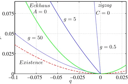
Unlike the Eckhaus instability, the zigzag instability is affected by the mean flow. Vorticity and mean flows act as a stabilizing influence on the zigzag instability, which is suppressed for larger values ofg, resulting in a larger region of stable stripes for q < 0 in the (µ, q) stabil-ity diagram. Figure 2 shows how the zigzag instabilstabil-ity boundary behaves for different values of g. Note that for large enoughg, it no longer forms the lower stability boundary except for very smallµ.

The zigzag and Eckhaus instabilities cross in parame-ter space whengandq are related by

g= 3(3(1 +q)

2 −1) 4q(1 +q)4_{(2 +q)},

where q < 0. Furthermore, when g _→ 0, we recover the standard result for the SHE without mean flow, and when g _{→ ∞}, we have µzigzag → µExistence. However,

even in this limit, for smallµand q, µzigzag is

V. LONG-WAVELENGTH INSTABILITIES: SKEW-VARICOSE

The skew-varicose instability, which is driven by the in-clusion of mean flow, the strength of which is determined by g, is associated with modes for which the maximum positive growth rate occurs whenk6= 0 andl 6= 0. Two conditions are required to characterize the SVI: the de-terminant should be zero and should have maximum or minimum value (for model 1 and model 2 respectively) fork6= 0 andl6= 0. We first express these conditions for the SVI in terms of the coefficientsA−Gof the expres-sion (14), the power series expanexpres-sion of the determinants ofJ1 andJ2, which we denote simply byDet. We then

express these conditions in terms of the parametersµ,q

and eitherg orgm,cand P r, in order to locate the SVI

boundary in the (µ, q) plane.

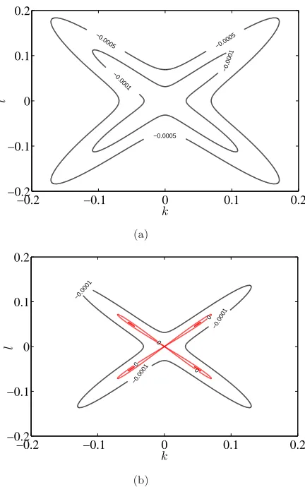
There are two different manifestations of the skew-varicose instability. In the first (case I), the instability emerges fromk=l= 0, as illustrated in figure 3. In this case, the determinant is negative for (k, l) close to (0,0), corresponding toA <0 andC <0. If we suppose in the first instance that we can write the leading order terms in the determinant as: Det=Ak

4 +Bk2

l2 +Cl4

+O((k2 +l2

)3

)

k2₊

l2 ,

then imposing Det = 0, along with ∂Det/∂k = 0 and

∂Det/∂l = 0, results in (B2

−4AC)(A₋B+C) = 0 and k2

l2 = B− 2C

B−2A. In order for k

2_/l2 _{to be positive, we}

needB > max(2A,2C), which excludes B=A+C and

B=−√4AC. We conclude that

B2₋4AC >0, A <0, C <0 andB >0 with k

2

l2 =

r C A

(15) is the condition for the SVI. However, the truncation of Det above is degenerate: the conditions are satisfied along a line in the (k, l) plane, rather than at a point. This degeneracy is resolved by restoring the higher order terms, as illustrated in figure 3.

The other possibility for the skew-varicose instability is that it can accompany the Eckhaus instability. This occurs when A > 0 andC < 0: for l = 0 and D < 0,

Detis positive for a range ofkand attains its maximum on the l = 0 axis at a finite k = kmax. In the (k, l)

plane, (kmax,0) can either be a maximum or a saddle, as

illustrated in figure 4. We define the SVI (case II) to be the point at which (kmax,0) changes from a maximum

to a saddle; at this point the maximum eigenvalue moves off thekaxis.

Unlike in the previous case, the growth rate at the SVI is positive, since stripes are already Eckhaus unsta-ble. Therefore the SVI occurs when there is a degenerate maximum atl = 0 andk=kmax, about to become

sad-dle. The conditions ∂Det

∂k2 = 0 and ∂Det

∂l2 = 0 at this point

yield the parameter values at which this variant of the skew-varicose instability occurs.

At l = 0, the first condition implies k2

max = −2AD +

O(A2_{), and the second condition implies (B}

−A) + (E₋

−0.0005

−0.0005 −0.0005

−0.0001

−0.0001

k

l

−0.2 −0.1 0 0.1 0.2 −0.2

−0.1 0 0.1 0.2

(a)

k

l

0

0

0

0

−0.0001

−0.0001

−0.0001

−0.2 −0.1 0 0.1 0.2 −0.2

−0.1 0 0.1 0.2

(b)

FIG. 3. (Color online) Case I of the SVI: behavior of theDet

in the (k, l) plane forA =−0.1 andC =−0.1 (A <0 and

C <0 makes stripes Eckhaus and zigzag stable). The other coefficients areD =−1, E = 2, F =−1 andG=−1. (a)

B= 0.195, giving stable stripes (B2<4AC). (b)B= 0.205, giving stripes that are unstable to the SVI (B2_{>4AC). The} positive maximum of the determinant emerges from (k, l) = (0,0) but occurs withk 6= 0 andl6= 0. A negative value of the determinant is indicated by black contours while zero and positive values of the determinant are in red(gray).

D) −A

2D

= 0 at k=kmax. Hence in the limit of small A, the condition for case II of the SVI is

B=

D+E

2D

A+O(A2), A >0 andD <0,

withk2₌ −A

2D +O(A

2_{) andl= 0. (16)}

Contours ofDet on either side of this boundary are il-lustrated in figure 4. Moreover, the conditions (15) and (16) are summarized in the schematic diagram in figure 5, which also indicates the regions affected by the SVI and the point (A, B) = (0,0), where the two cases coincide.

0

0

0

0

k

l

5e−006

5e−006 5e−006

−1e−005

−1e−005

−0.08 −0.04 0 0.04 0.08

−0.02 0 0.02

(a)

k

l

0

0

0 5e−006

5e−006

5e−006

−1e−005

−1e−005

−0.08 −0.04 0 0.04 0.08

−0.02 0 0.02

(b)

FIG. 4. (Color online) Case II of the SVI: behavior of theDet

in the (k, l) plane forA = 0.005 and C =−0.1 (A >0 and

C <0 makes stripes Eckhaus unstable but stable to zigzags). The other coefficients areD=−1,E= 2,F =−1 andG=

−1. (a)B=−0.003, giving SV stable and Eckhaus unstable stripes B <D+E

2D A

; the maximum occurs with l= 0. (b)

B=−0.001, giving stripes that are unstable to both SV and Eckhaus instabilities B > D+E

2D A

; the maximum moves off axis, and (kmax,0) is now a saddle. A negative value of the

determinant is indicated by black contours while zero and positive values of the Determinant are in red (gray).

bifurcation lines we have used a branch-following pack-age, MATCONT [31]. An example of the calculation for model 2 is given in figure 6, which was computed work-ing directly with numerically determined eigenvalues and computing ∂

∂k2 and ∂

∂l2 numerically. In case I, the SVI

boundaries derived using condition (15) coincide with the numerical computation. However, in case II, condition (16) agrees with the numerical computation only when

Ais close to zero, as would be expected. The transition from case I to case II occurs at (µ, q) = (0.1367,0.2387) forg = 0.5: for smallerµ, the stability region of stripes is bounded on the right by the Eckhaus instability, while for largerµ, the Eckhaus instability is preempted by the SVI. Forg= 5, the SVI pre-empts the Eckhaus instabil-ity for allµ.

0 0

A

B

<

0

B

B

>

0 SVI for case I

A >0

A <0

B2_{= 4AC}

SVI unstable stripes

Eckhaus unstable stripes

Eckhaus

stable stripes

SVI for case II

B=¡D+E 2D

¢

A

FIG. 5. (Color online) Schematic diagram of the conditions for the Eckhaus and SV instabilities in cases I and II in (A, B) plane. The Eckhaus instability occurs whenA = 0 (dashed red line). The blue curve shows the SV stability boundary:

B2 _{= 4AC in case I (A <0), and B =} D+E

2D A

in case II (A >0). At the intersection of the two stability boundaries, (A, B) = (0,0).

0 0.05 0.1 0.15 0.2 0.25 0

0.05 0.1 0.15 0.2 0.25

q

µ

Eckhaus

Existence SV, g= 0.5

SV, g= 5

FIG. 6. (Color online) Numerical computation (in model 2) of the SV stability boundary in the (µ, q) plane. For

g = 5, the SVI pre-empts the Eckhaus instability for all

µ and hence the region of stable stripes is bounded by the skew-varicose instability curve. However, for g = 0.5, the region of stripe stability is bounded by the skew-varicose in-stability curve only when µ > 0.2387. The crossing point, (0.1367,0.2387), of the two boundaries is denoted as a red square. For 0 < µ <0.2387, the Eckhaus precedes the SV curve, which reaches the origin as a parabolaµ= 9.33q2_{. The} green thick curve denoted by E is for the Eckhaus boundary whereas the dashed red curve is the boundary of existence of stripes.

log10(q)

µ

/µ

E

x

i

s

t

e

n

c

e

10−3 10−2 10−1 2.8

3 3.2

3.4 _{SV, g= 5}

Eckhaus

(a)

log10(q)

µ

/µ

E

x

i

s

t

e

n

c

e

10−4 10−3 10−2 10−1 2.4

2.6 2.8 3

B

Eckhaus

(A, B) = (0,0)

SV, g= 0.5

A

(b)

FIG. 7. (Color online) Numerical computation (in model 2) of the SVI boundary as a function of µ/µExistence and

log₁₀(q). µExistence= (1−(1 +q)2)2. The Eckhaus

bound-ary,A= 0, is denoted by a green thick curve and the shaded region corresponds to stable stripes. (a) g = 5 > gcritical.

Here, µSV/µExistence → 3 as q → 0. The SVI precedes

the Eckhaus for all q values. (b)g = 0.5 < gcritical. Here,

µSV/µExistence →2.3333 asq →0, which in turn becomes

µSV → 9.3333q2 as q → 0. The point of intersection of

the SVI boundary with the Eckhaus boundary is denoted by (A, B) = (0,0). A schematic illustration of theAandB axes at the crossing point is also shown (see figure 5).

for someg, saygEck, which is given by

gEck =

3 8

3(1 +q)2 −1 (1 +q)6

.

The condition A = 0 could be used to express gEck as

a function of µ if desired. In the limit µ → 0 and

q → 0, gEck goes to 0.75, which we call gcritical. The

expression for gEck and the value gcritical = 0.75 is

the same in models 1 and 2 provided we use the

rela-tion g = gm/(P r c2). The Eckhaus instability precedes

the SVI for some range of µ only if g < gcritical. We

have found that the SVI boundary for g > gcritical

ap-proaches the origin as µ = 12q2_{, as does the Eckhaus}

curve, whilst it approaches asµ=nq2_{, with 4< n <12}

wheng < gcritical. A detailed presentation of this

asymp-totic result will be discussed in section (V A). The dis-tinction between g > gcritical and g < gcritical is

illus-trated in figure 6 where we present SVI boundaries for

g= 5> gcriticalandg= 0.5< gcritical.

Interestingly, for a fixed q, g → 0 implies µSV → µExistence. Therefore when g → 0, the SVI boundary

coincides with the existence curve of stable stripes for smallµ.

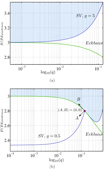
The Eckhaus and SVI boundaries are often very close, so we present our result in an alternative way in figure 7. Figures 7(a) and 7(b) present the SVI boundaries for

g= 5 andg= 0.5 in the (µ/µExistence , log10(q)) plane.

This is a better way of illustrating the regions of stable stripes (shaded regions) and the behavior of the Eckhaus and SVI boundaries asq → 0. Moreover, it shows how the coordinates axesA and B from (14) can be defined near the SVI–Eckhaus crossing point.

A. Asymptotic analysis of the SVI boundary

In this section we focus on the asymptotic behavior of the SVI boundary in model 2, in the two cases discussed above, g > gcritical and g < gcritical. Let us consider

the case when g > gcritical, where the SVI boundary

pre-empts the Eckhaus instability boundary. We use the conditionB2

−4AC= 0, which can be written as

F1g2+F2g+F3= 0, (17)

where theFi’s are functions of µand q. In the limit of

very smallµand q,

F1≈

1

9(16384q

6

−8192µq4_{+ 1024µ}2_q2

−256µ3_{q+ 16µ}4_),

(18a)

F2≈

1

3(−24576q

5_{+ 8192µq}3

−512µ2q₋64µ3), (18b)

F3≈(9216q4−1536µq2+ 64µ2). (18c)

We note at this point that equation (17) is valid for model 1 (with the same values of F1, F2 and F3) when

we identify g with gm/P r c2. For smallish g ≥gcritical,

as µ → 0, µ ∼ q2 _{as shown in figure 7(a) and hence}

functions in equation (18) can be taken asF1∼q6,F2∼

q5 _{and F}

3 ∼ q4. Therefore the equation (17) can be

approximated asF3 = 0, in which case µ= 12q2. This

can be improved by includingF2and henceF2g+F3= 0

in which case we obtain

µSV = 12q2

9−8qg

9−24qg

,(g > gcritical, q≪1/g) (19)

and hence µ _→ 12q2 _{when q}

→ 0. Therefore when

g > gcritical, the SVI boundary for smallµhas the same

10−5 10−4 10−3 10−2 10−4

10−2

log10(q)

log

1

0

(

µ

)

µ= 12q2

µ= 8q

g= 103

g= 104

g= 105

g= 107

g= 10

g= 102

FIG. 8. (Color online) Numerical computation of the SVI boundary on a logarithmic scale forg= 10i

fori= 1,2,3,4,5 and 7. The transition from µ ∼ q to µ ∼ q2 occurs when

g ∝ 1/q. In the limit of small q, the SVI curve is tangent to µ = 12q2_{, whereas in the limit of largeg, the SVI curve} goes asµ∼8q asµincreases. Both asymptotes,µ∼8qand

µ∼12q2 _{are denoted by red thick lines.}

is also of interest, as it corresponds to stress-free bound-ary conditions (see section (VI) below). In this limit, we expect the SVI boundary (as shown in figures 14 and 16 below) should haveµ∼q[19]. From equation (18) with

µ _∼ q, we have F1 ∼ q4, F2 ∼ q3 and F3 ∼ q2 and F1g2+F2g+F3 ∼ q2 q2g2+qg+ 1

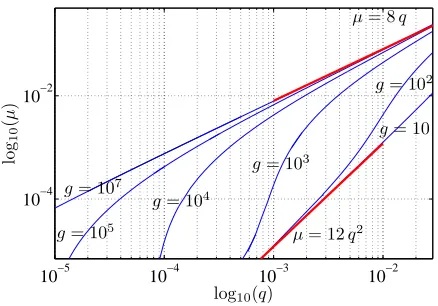
. If qg _≪ 1, we set F3 = 0 and recover µ = 12q2. If qg ≫ 1, we set F1= 0 and obtainµ∼8q. Again, this can be improved

by settingF1g+F2= 0, and we obtain

µSV = 8q

2qg+ 3 2qg₋3

,(g > gcritical, q≫1/g). (20)

Finally, we note that the transition between µ ∼ 12q2

and µ ∼ 8q will occur when qg is of order unity, so

qtransition ∼ 1_g. These three regimes are illustrated in

figure 8.

In the skew-varicose mechanism for g > gcritical, the

maximum ofDetis attained for perturbations of a mode, say (kmax, lmax), askmax→0 and lmax→0. As shown

by the equation (15), kmax 2

lmax 2 =

q C A and so

kmax

lmax =O(1).

Secondly, let us consider the case g < gcritical, for

which the SVI boundary lies in the Eckhaus band for small µ. We do not have an exact criterion for the SVI in this case, though equation (16) is an approximate cri-terion. However, for smallµ, we expect µSV to depend

approximately linearly on g. We know from equation (19) that for g = gcritical, µSV → 12q2 as q → 0 and

from conditions in equation (16) in the limitg _→0, we have µSV → 4q2 as q → 0. A linear interpolation

be-tween these yields

µSV ≈4

2

gcritical

g+ 1

q2,(g < gcritical, q≪1).

(21) This relation is shown numerically using MATCONT [31] to be a very good approximation; µSV/µExistence

be-haves linearly with g with a gradient 8/3. In addition, the numerical simulation illustrated in figure 7(b), shows at g = 0.06, µ/µExistence → 2.6 as q →0 which agrees

well with equation (21). All these explicit results are for model 2. When g > gcritical, the expressions for

con-ditions given in (15) are the same for model 1 with the relation g = gm/P r c2. Therefore, equations (19) and

(20) are the same for model 1. When g < gcritical, for

model 1, the condition for the SVI given by equation (16)

withg=gm/P r c2 is not the same as in model 2.

How-ever, for fixedP randc6= 0, we find thatµSV/µExistence

behaves linearly withgm and hence equation (21) holds

for model 1. The case wherec = 0 is considered in the next section.

VI. LONG-WAVELENGTH INSTABILITIES:

SKEW-VARICOSE AND OSCILLATORY SKEW-VARICOSE WITH STRESS-FREE

BOUNDARY CONDITIONS.

We now consider the case that models convection with stress-free boundary condition. In model 1,c is the pa-rameter that accounts for the boundary conditions at the top and bottom, and stress-free boundary conditions cor-respond toc = 0. Using the relation g = gm/P r c2 to

connect the two models, taking the limit g _{→ ∞} corre-sponds to stress-free boundary condition in model 2.

When c = 0, for any coupling constant gm, the SVI

boundary always pre-empts the Eckhaus boundary in the (µ, q) plane. To show this we can focus on model 1, for which the SVI condition isF1gm2+F2gmP r c2+

F3(P r c2)2 = 0 with F1, F2 and F3 given in equation

(18); this confirms the relation g = gm/P r c2. Hence c = 0 implies F1 = 0, and this gives the criterion for

instability asµ= 8qfor anygm, as above. A remarkable

property of the SVI in model 1 with stress-free boundary conditions is that the stability boundary is independent ofP r andgm.

Another instability of interest in the stress-free case is the oscillatory skew-varicose (OSV) instability, which consists of a long-wavelength transverse oscillations of the stripes that propagate along their axis [18]. For OSV modes, the associated eigenvalues are complex. This in-stability does not occur in model 2 becauseT r(J2)<0

−0.1 −0.05 0 0

0.05 0.1 0.15 0.2 0.25 0.3

µ

q

gm= 1000

gm= 100

gm= 25

Existence

gm= 5

Eckhaus

gm= 1

FIG. 9. (Color online) The location of the OSV instability boundary for model 1 for c= 0 (stress-free boundary condi-tions), P r = 1 andgm= 1000,100,25,5 and 1. Stripes are

OSV unstable to the left of the OSV boundary. For smallµ, the boundary is asymptotic toµ=−3+√5

3

qgm. The

Eck-haus boundary is denoted in green thick and the existence curve is in dashed red.

We derive the asymptotic behavior of the OSV insta-bility boundary. At the point of instainsta-bility, the eigen-values are purely imaginary; this gives two conditions,

C−AB = 0 and B >0, where the characteristic equa-tion ofJ1isλ3+Aλ2+Bλ+C= 0. The coefficientsA, B andC are functions ofgm,q,µ,kand l. We have set P r= 1 for illustrating this calculation. For small k and

l, the conditionC−AB = 0 gives,

G1

gmq µ

2

+G2

gmq µ

+G3= 0, (22)

after maximizingC₋AB over (k, l). TheGi’s are

func-tions of µandq. In the limit of very smallµand q, we find,

G1≈

1

9 1024−8192

q2

µ

+ 16384

q2

µ 2!

, (23a)

G2≈512−

26624 3

_q2

µ

+ 46421

_q2

µ 2

−76459

_q2

µ 3

,

(23b)

G3≈256−8192

_q2

µ

+ 90112

_q2

µ 2

−393216

_q2

µ 3

+589824

q2

µ 3

, (23c)

where we have dropped terms that can be shown to be smaller than those retained.

We note at this point that equations (22) and (23) with (q2_/µ)

≪ 1 give 1024 9

gmq

µ 2

+ 512gmq µ

+ 256 = 0,

which impliesµ=−3+₃√5qgm. Hence, the OSV

insta-bility boundary has a linear relationship betweenqandµ

−0.10 −0.05 0 0.05 0.1 0.15 0.05

0.1 0.15 0.2 0.25 0.3

q

µ stable stripes

SV, g= 50

Existence Eckhaus

FIG. 10. (Color online) Stability diagram in the neighborhood ofµ = 0 for model 1 with c2 _{= 2 (no-slip boundary} condi-tions), P r= 1, gm = 50 andγ = 2.5. Stable stripes are in

the region indicated, bounded by Eckhaus instability (green thick curve) from below and by the SVI boundary (blue thin curve) from above.

for smallµ, and it bounds the region of stable wavenum-bers for negativeq. Stripes are stable on the right of the boundary. In this asymptotic limit, the point of max-imum growth rate in the (k, l) plane can be found at the point of maximum of C ₋AB; this point satisfies

l/k=√5. Figure 9 shows the behavior of the OSV in-stability boundary in model 1 with c = 0, for different values of the coupling constantgm.

When c is increased from zero, the OSV instability turns into the so-called oscillatory instability [32]. This has the nature of an oscillatory cross-roll instability, set-ting in with non zero k and l. The boundary of this oscillatory instability emerges fromβ = 0, the existence curve. However, this instability is prominent only for

P r c2

≪ 1; for higher values of P r c2_{, the instability}

moves to larger negativeq.

VII. SHORT-WAVELENGTH INSTABILITIES:

THE CROSS-ROLL INSTABILITY.

The cross-roll (CR) instability is so-called because the fastest growing disturbances appear to take the form of stripes perpendicular to the basic steady stripe pattern: these disturbances have non-zerokandlin the limitµ_→

0 [30]. In contrast to the oscillatory cross-roll instability discussed above, the most unstable eigenvalue at the CR instability is zero.

We will show numerically in section (VIII) below that the CR instability only forms a boundary of the region of stability of stripes ifg is large. The filtering _Fγ,

−6 −4 −2 0 2 4 6 x 10−3 0

0.2 0.4 0.6 0.8

1x 10

−3

q

µ

Eckhaus

zigzag

Existence

CR

(f)

(e) (d)

(c) (b) SV (a) stable stripes

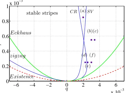
FIG. 11. (Color online) Stability diagram in the neighborhood of µ = 0 for model 1 withc2 _{= 2 (no-slip boundary} condi-tions), P r = 1, gm = 1000 andγ = 2.5. Stable stripes are

in the region indicated, bounded by the SV and CR instabil-ities from above, and by the zigzag and Eckhaus instabilinstabil-ities from below. Stable stripes exist atq= 0 for range ofµclose to zero. Growth rates as a function ofk and lat the points indicated by (a)–(f) are given in figure 12.

andq, asymptotic analysis of the type carried out above cannot be done. Numerical examples are shown in the next section.

VIII. NUMERICAL ILLUSTRATION OF

COMBINED STABILITY BOUNDARY.

We now present numerical results obtained with MAT-CONT [31]. Details of the specification of the conditions on the eigenvalues for each of the six types of instability are given in the Appendix. We choose two illustrative parameter values: gm= 50 and gm= 1000, and we

con-sider no-slip (c2 _{= 2) and stress-free (c = 0) boundary}

conditions.

Figure 10 shows the stability diagram for model 1 with parameter valuec2_{= 2 (corresponding to no-slip}

bound-ary conditions), P r = 1, gm= 50 and γ = 2.5. The

re-gion of stable stripes is bounded by the SVI from above and the Eckhaus instability from below. The zigzag in-stability boundary for this value ofgmlies below the left

Eckhaus boundary except for very small µand q (as in figure 2). The CR instability does not occur in this range of parameters.

Figure 11 and 13 show the stability diagram for model 1 with parameters c2 _{= 2 (no-slip), P r = 1, g}

m = 1000

andγ= 2.5. Close toµ= 0 (figure 11), a neighborhood of q = 0 is in the stable regime and the zigzag and the SV instabilities bound the region of stable stripes. For

µ >5_×10−4_{, the region of stable stripes is bounded by}

the CR instability from above and by the Eckhaus insta-bility from below. For this value ofgm, the CR instability

boundary crosses the SVI boundary, and the zigzag in-stability boundary has a linear behavior for smallµ.

For the same parameter values, the stability diagram

for a larger range ofq andµis shown in figure 13. The region of stable stripes is bounded by the Eckhaus in-stability from below and the CR inin-stability from above. The zigzag instability boundary lies close to the existence curve and is of less interest for this value ofgm.

Figure 12 shows the eigenvalue behavior at selected points in the (q, µ) space from figure 11, as a function of (k, l), showing how stripes can be unstable to one or both of the SV and CR instabilities. We note that the CR in-stability occurs for reasonably large values of k _≈ 0.04 and l _≈0.2. In contrast, in the SVI, contours of posi-tive growth rate emerge from (k, l) = (0,0). When both instabilities exist, two separate peaks of growth rates ap-pear. For largeq, these contours can join to form one large contour.

We have computed the stability diagrams for model 2 with g = 500 and g = 25, and these are qualitatively the same as 10 and 11, consistent with the relationg =

gm/P r c2.

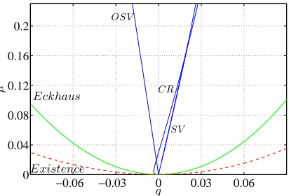
Figure 14 and 16 similarly show the instability bound-aries for model 1, with parametersc= 0 (corresponding to stress-free boundary conditions),P r= 1,γ= 2.5 and

gm= 50 and gm= 1000. The results agree qualitatively

with earlier calculations by Bernoff [19], who found a similar linear relation betweenµ and q for the SV and OSV instabilities in convection with stress-free boundary conditions; he did not consider the CR instability.

Disregarding the CR instability, stripes would be sta-ble between the OSV instability and SVI boundaries. However, as seen in figure 14, the SVI is always pre-empted by the CR instability; these boundaries appear to be parallel for largerµ. Forµ <0.32, there are no sta-ble stripes. For higherµ, the stable region is bounded by the CR instability from above and by the OSV instability from below.

Figure 15 shows the change of structure of the eigen-values when moving from left to right in the stability diagram shown in figure 14. At µ = 0.1, we selected four different wavenumbers: q = −0.05, where stripes are OSV unstable,q=₋0.02, where stripes are CR and OSV unstable,q= 0.0058, where stripes are CR unstable but OSV stable andq= 0.05, where stripes are CR and skew-varicose unstable, though the distinction between these two instabilities has become blurred.

Figure 16 presents instability boundaries for stress-free boundary conditions withP r= 1,gm= 50 andγ= 2.5.

This provides an illustration of the change of the CR instability boundary with gm. For gm = 50, the CR

instability boundary crosses the SVI boundary and the effect of the CR instability is reduced.

A. Curious behavior of growth rates

0

k

l

0 0.02 0.04 0.06

0 0.05 0.1 0.15 0.2 0.25 0.3

(a)

0

0

k

l

0 0.02 0.04 0.06

0 0.05 0.1 0.15 0.2 0.25 0.3

(b)

k

l

0 0

0 0.02 0.04 0.06

0 0.05 0.1 0.15 0.2 0.25 0.3

(c)

0

0

k

l

0 0.02 0.04 0.06

0 0.05 0.1 0.15 0.2 0.25 0.3

(d)

k

l

0

0

0 0.02 0.04 0.06

0 0.05 0.1 0.15 0.2 0.25 0.3

(e)

0

k

l

0 0.02 0.04

0 0.05 0.1 0.15 0.2 0.25 0.3

(f)

FIG. 12. (Color online) Growth rates of perturbations at selected (µ, q) indicated by (a)–(f) in figure 11. (a)µ= 8.5×10−4_,

q= 0.002; stripes are CR unstable, but growth rates forkandlclose enough to zero are negative. (b)µ= 5.5×10−4_{,q= 0.003;} stripes are CR and SV unstable. Growth rates fork andlclose enough to zero become positive due to the SVI and there are two distinct zero contours. (c) µ = 5.5×10−4_{,q = 0.0034; stripes are CR and skew-varicose unstable. One large contour} encloses both the SV and CR instabilities. (d) µ= 2.5×10−4_{,q = 0.00225; stripes are skew-varicose unstable, and growth} rates forkandlclose enough to zero are positive for a range of polar angles. (e)µ= 2.5×10−4_{,q= 0.0025; same as case (b),} but the maximum occurs in the SV region. (f)µ= 2.5×10−4_{,q= 0.003; same as case (c), but again the maximum occurs in} the SV region. The zero contour is denoted in black (outer) and contours of positive growth rate are denoted in red (inner in gray).

q

µ

−0.06 −0.04 −0.02 0 0.02 0.04 0.06 0

0.01 0.02 0.03 0.04 0.05 0.06

Existence zigzag

SV CR

Eckhaus

FIG. 13. (Color online) Stability diagram with parameters as in figure 11 covering a larger range of q and µ. Stripes are stable in the shaded region, bounded by the Eckhaus and CR instabilities.

These instabilities occur even in the SHE and so are not related to presence of the mean-flow. They have not been studied before, though they are of less interest since they do not bound the region of stable stripes. We consider

q

µ

−0.10 −0.05 0 0.05 0.1

0.1 0.2 0.3 0.4

(a)

Existence

(b) (c) (d)

CR

OSV _SV

Eckhaus

FIG. 14. (Color online) Stability diagram for model 1 with

c= 0 (stress-free boundary conditions), P r= 1, gm = 1000

k

l

0.09

0

0 0.2 0.4 0.6

0 0.1 0.2 0.3 0.4 0.5 0.6

(a)

k

l

0

0

0.05

0 0.2 0.4 0.6

0 0.1 0.2 0.3 0.4 0.5 0.6

(b)

k

l

0

0

0.17

0 0.2 0.4 0.6

0 0.1 0.2 0.3 0.4 0.5 0.6

(c)

k

l

0 0

0.41

0 0.2 0.4 0.6

0 0.1 0.2 0.3 0.4 0.5 0.6

(d)

FIG. 15. (Color online) Growth rates of perturbations at selected (µ, q) indicated in figure 14, all with µ = 0.1. (a)

q =−0.05, where stripes are OSV unstable. (b)q =−0.02, where stripes are CR and OSV unstable. (c) q = 0.0058, where stripes are CR unstable but OSV stable. (d)q= 0.05, where stripes are CR and skew-varicose unstable, though the distinction between these two instabilities has become blurred. The zero contour of the real part of the eigenvalue is denoted in black (outer) and contours of positive growth rate are in red (inner in gray). The eigenvalues in the OSV case are complex.

them briefly here.

Contours of the growth rates of perturbations for se-lected parameter values are shown in figure 17. As shown in figure 17(a), for a fixed smallµ, when q is increased from the left existence boundary (q < 0), modes ap-proximately in an annulus of unit radius centered at (k, l) = (1 +q,0) have positive real eigenvalues in addi-tion to unstable modes for smallk andl, corresponding to the Eckhaus and zigzag instabilities. This annulus dis-appears for largerqleaving only the Eckhaus and zigzag unstable modes close to (k, l) = (0,0), as shown in fig-ure 17(b). This process is in part reversed for q > 0 going towards the right existence boundary: here modes are Eckhaus unstable only, but for large enough q, the annulus of unstable modes reappears. The behavior of growth rates in the right Eckhaus band is illustrated in figure 17(c) and 17(d).

We have confirmed that this curious behaviour is not a result of using the projection operatorPαin the Swift–

Hohenberg equation.

−0.06 −0.03 0 0.03 0.06

0 0.04 0.08 0.12 0.16 0.2

q

µ

OSV

Eckhaus CR

SV

Existence

FIG. 16. (Color online) Stability diagram for model 1 with

c= 0 (stress-free boundary conditions),P r= 1,gm= 50 and

γ= 2.5. Stable stripes exist forµ >0.02; the region of stable stripes is bounded by the OSV boundary on the left and the CR boundary and then the SV on the right.

IX. ANALYSIS OF THE ROLE OF

MEAN-FLOWS

We now illustrate the stability diagrams in a different manner. For a fixedµ, we show how the coupling to the mean flow affects the region of stable stripes. This choice of presentation provides useful information for numerical simulations of the PDEs in large domains. Figure 18 represents the region of stable stripes for model 2 in the

(g, q/√µ) plane forµ= 0.1. We chooseq/√µas the

coor-dinate for ease of comparison between different values of

µ. Figure 18(a) shows the stability diagram for smallg, where the region of stable stripes is bounded from above by the Eckhaus instability forg <0.574 and by the SVI

forg >0.574, and by the zigzag instability from below.

Figure 18(b) shows how for largeg, the region of stable stripes is bounded by the CR instability from above and by the Eckhaus instability from below, and the region is eliminated wheng&2_×104_{. Figure 19 shows the}

loca-tion of the CR instability forµ= 0.01,0.001 and 0.0001. The upper bound ongbeyond which there are no stable stripes initially decreases withµand then increases. The behavior of model 1 is qualitatively the same.

Figure 20 presents stability diagrams for model 1 with

c= 0 (stress-free boundary conditions), forµ= 0.1 and

µ= 0.01. The SV and the OSV instabilities bound the region of stable rolls from above and below and the CR instability makes the upper bound ongm. Stable stripes

exists only for smallgmand the upper bound ongm

fur-ther reduces withµ.

X. CONCLUSION

k

l

0 0.5 1 1.5 2

0 0.2 0.4 0.6 0.8 1 1.2

(a)

k

l

0 0.5 1 1.5 2

0 0.2 0.4 0.6 0.8 1 1.2

(b)

k

l

0 0.5 1 1.5 2

0 0.2 0.4 0.6 0.8 1 1.2

(c)

k

l

0 0.5 1 1.5 2

0 0.2 0.4 0.6 0.8 1 1.2

(d)

FIG. 17. (Color online) Growth rates of perturbations as a function of (k, l) for the Swift–Hohenberg equation (1), with

ψ3 _{replaced by P}

α(ψ3). Figures (a) and (b) correspond to

points in the left Eckhaus band,q <0, whereas (c) and (d) correspond to points in the right Eckhaus band, q >0. (a) Stripes are zigzag and Eckhaus unstable and the unstable modes lie approximately in a annulus of unit radius centered at (k, l) = (1 +q,0) have positive real eigenvalues. (b) Stripes are zigzag and Eckhaus unstable. (c) Stripes are Eckhaus unstable. (d) Stripes are Eckhaus unstable and in addition, an annulus of unit radius centered at (k, l) = (1 +q,0) has positive real eigenvalues. Thick black: zero contour. thick Red (inner in gray): positive contour. Dotted curve: circle of unit radius centered at (k, l) = (1 +q,0).

vorticity has its own independent dynamics [7]. In the second, vorticity is directly slaved to the order param-eter [26]. These two models are related to each other through g = gm/(P r c2), wheregm and g are the

cou-plings to mean flow in model 1 and model 2 respectively. Two boundary conditions were considered in this work: stress-free (c= 0) and no-slip (c2_{= 2).}

In order to explore long-wavelength instabilities, we carried out a complete linear stability analysis of stripes. We expressed the relevant determinants as power series ink2 _andl2_{, where (k, l) is the perturbation wavevector.}

We were able to derive explicit expressions for the largest growth rates in most cases. This has led to an improved understanding of the instabilities of stripes. Unlike in previous work [19, 23, 28], we have not had to make as-sumptions on the relation betweenk,land the amplitude

0 2 4 6 8 10

−0.5 −0.25 0 0.25 0.5

g

q/

√

µ

SV

zigzag

Existence Eckhaus

(a)

0 0.5 1 1.5 2

x 104 −0.5

−0.25 0 0.25 0.5

g

q/

√

µ

Existence SV

zigzag

CR

Eckhaus

(b)

FIG. 18. (Color online) Stability diagrams in (g, q/√µ) plane for model 2 withµ = 0.1 and γ= 2.5. (a) For smallg: the region of stable stripes is mainly bounded by zigzag and SV instabilities. (b) For large g, the region of stable stripes is bounded by the Eckhaus (thick green) and CR instabilities. These instability boundaries cross aroundg= 2×104, elimi-nating the region of stable stripes. The region of stable stripes is hatched.

of the basic stripe solution. This approach has been made possible through the use of the projection operator,Pα,

which allows the exact stripe solution to be written down easily [29].

The skew-varicose instability, which was our main con-cern, has two different behaviors: if stripes are stable to the Eckhaus instability, in the limit of µ = 0, the SVI goes asµ∼12q2_{, providedg >0.75. The most unstable}

wavevector satisfiesk2_/l2_{=O(1). Forg <0.75, the SVI}

boundary crosses the Eckhaus curve, and in the limit of

µ= 0, it goes asµ_∼aq2 _{with 4< a <12. In model 1,}

the criticalgm is 0.75P r c2. In the largeglimit (that is,

for very lowP r, or for stress-free boundary conditions), there is a transition of the SVI boundary fromµ= 12q2

toµ= 8qat a wavenumber satisfying q_∝1/g.

An additional instability, the oscillatory skew-varicose (OSV) instability, is encountered for stress-free boundary conditions in model 1. The OSV instability boundary is approximatelyµ=−3+√5

3

0 500 1000 1500 2000 −0.5

−0.25 0 0.25 0.5

g

q/

√

µ

CR SV

Eckhaus

Existence zigzag

(a)

0 500 1000 1500 2000

−0.5 −0.25 0 0.25 0.5

g

q/

√

µ

zigzag SV

CR

Existence Eckhaus

(b)

0 500 1000 1500 2000

−0.5 −0.25 0 0.25 0.5

g

q/

√

µ

SV

CR

Existence

zigzag

Eckhaus

(c)

FIG. 19. (Color online) Stability diagrams in (g, q/√µ) plane for model 2 with γ = 2.5. (a) µ = 0.01 (b) µ = 0.001 (c)

µ= 0.0001. In all three cases CR instability reduces the region of stable stripes which is hatched.

0 200 400 600 800 1000

−0.5 −0.25 0 0.25 0.5

gm

q/

√

µ

Eckhaus

Existence CR SV

OSV

(a)

0 50 100 150 200

−0.5 −0.25 0 0.25 0.5

gm

q/

√

µ

OSV

CR SV

Existence Eckhaus

(b)

0 50 100 150 200

−0.5 −0.25 0 0.25 0.5

gm

q/

√

µ

Eckhaus

SV

Existence CR OSV

(c)

FIG. 20. (Color online) Stability diagrams in (gm, q/õ) plane with c = 0 (stress-free boundary conditions), P r = 1 and

γ= 2.5. (a)µ= 0.1 and for largegm: (b)µ= 0.1 and for smallgm: stable stripes are completely eliminated whengm&130.

(c)µ= 0.01 and for smallgm. In all three cases, the region of stable stripes (hatched ) is mainly bounded by the OSV, SV

and CR instabilities, and the CR instability makes the upper bound ingm and reduces the region of stable stripes withµ.

We confirmed our analytical results by numerical computations of the eigenvalues of the stability matri-ces. These eigenvalues also allow us to explore short-wavelength instabilities: cross-roll and the oscillatory in-stability. Finally, we have shown how the region of stabil-ity of stripes is eliminated for smallµ and large enough

g.

The use of the projection operatorPα, which is

equiva-lent to a truncation to selected wave numbers, made this analysis straightforward and allowed the complete un-derstanding of the skew-varicose instability in our mod-els. Numerical simulations of these projected models for smallµ have qualitatively the same solutions as the un-projected PDEs (for example, they have SDC solutions); this is our justifcation for using these projected models in the stability analysis for small µ. The projected and unprojected models will of course differ for largeµ. It is of interest to address the question whether a similar pro-jection could be used in the analysis of the Navier-Stokes equations.

We finally comment on the implications of our analy-sis on the direct numerical simulations of PDE’s in large domains. The most striking signature of the inclusion of

a mean-flow is the existence of the skew-varicose insta-bility, which can play an important role in the formation of the spiral defect chaos or defect chaos [12, 14]. Hence the improved understanding of the stability of stripes in this work provides a foundation for numerical simula-tions of spiral defect chaos and defect chaos. The SDC state exists inside the Busse balloon, where convection rolls are stable [1]. Thus we intend in a future paper to relate the SDC and defect chaotic states present in these generalized SH models to calculations carried out using Rayleigh–B´enard convection with stress-free [1] and no-slip [5] boundary conditions, aiming to improve the understanding of why SDC occurs in convection. The results of this work provide useful information for the choice of parameters for different instability regimes in model 1 and model 2. In particular we will be interested in numerical simulations with small µ and in large do-mains. This work also justifies using model 2 with large