Testing R-parity with geometry

City, University of London Institutional Repository

Citation

:

This is the published version of the paper.

This version of the publication may differ from the final published

version.

Permanent repository link:

Link to published version

:

Copyright and reuse:

City Research Online aims to make research

outputs of City, University of London available to a wider audience.

Copyright and Moral Rights remain with the author(s) and/or copyright

holders. URLs from City Research Online may be freely distributed and

linked to.

JHEP03(2016)079

Received_{: December 8, 2015}

Accepted_{: February 29, 2016}

Published_{: March 14, 2016}

Testing R-parity with geometry

Yang-Hui He,a,b,c Vishnu Jejjala,d Cyril Mattia,d and Brent D. Nelsone

a

Department of Mathematics, City University, London, Northampton Square, London EC1V 0HB, U.K. b

School of Physics, NanKai University, 94 Weijin Road, Tianjin, 300071, P.R. China c

Merton College, University of Oxford, Merton Street, OX1 4JD, U.K. d

Mandelstam Institute for Theoretical Physics, NITheP, and School of Physics, University of the Witwatersrand,

1 Jan Smuts Avenue, Johannesburg, WITS 2050, South Africa e

Department of Physics, Northeastern University, 360 Huntington Avenue, Boston, MA 02115, U.S.A.

E-mail: [email protected],[email protected], [email protected],[email protected]

Abstract: _{We present a complete classification of the vacuum geometries of all}

renor-malizable superpotentials built from the fields of the electroweak sector of the MSSM. In addition to the Severi and affine Calabi-Yau varieties previously found, new vacuum man-ifolds are identified; we thereby investigate the geometrical implication of theories which display a manifest matter parity (or R-parity) via the distinction between leptonic and Higgs doublets, and of the lepton number assignment of the right-handed neutrino fields.

We find that the traditional R-parity assignments of the MSSM more readily accommo-date the neutrino see-saw mechanism with non-trivial geometry than those superpotentials that violate R-parity. However there appears to be no geometrical preference for a fun-damental Higgs bilinear in the superpotential, with operators that violate lepton number, such as νHH, generating vacuum moduli spaces equivalent to those with a fundamental bilinear.

Keywords: _{Supersymmetric Effective Theories, Supersymmetric gauge theory}

JHEP03(2016)079

Contents

1 Introduction 1

2 Gauge invariant operators and syzygies 4

3 F-terms constraints 8

3.1 Cases with two elemental trilinears 9

3.2 Cases without any elemental trilinear 9

3.3 Cases with only one elemental trilinear 10

3.3.1 LHe 10

3.3.2 LLe 12

4 Right-handed neutrinos 16

4.1 Cases with two elemental trilinears 17

4.2 Cases without any elemental trilinear 17

4.3 Cases with only one elemental trilinear 19

4.3.1 LHe 19

4.3.2 LLe 20

4.4 Majorana mass term 21

5 Discussion and outlook 24

1 Introduction

The vacuum of anN = 1 supersymmetric quantum field theory consists of field configura-tions that satisfy the F-term and D-term constraints. Recent advances in understanding the vacuum moduli space of the minimal supersymmetric Standard Model (MSSM) estab-lish that non-trivial geometrical characteristics correlate to specific parameter choices of the theory such as the number of generations of matter fields, the number of pairs of Higgs doublets, and the vanishing of coupling constants [1–4]. These are the first hints that a bot-tom up strategy to studying low dimensional effective field theories might yield information about the structure of its higher energy completion [5]. Frequently, the vacuum geometries of semi-realistic quantum field theories have interesting mathematical properties. They may, for instance, be Calabi-Yau, as happens for orbifolds ofC3 _{by discrete subgroups of} SU(2) and SU(3) [6] or for supersymmetric QCD (SQCD) [7].

JHEP03(2016)079

this series has conclusively demonstrated that special geometrical structure, such as simple embedding maps from one projective space to another, are rare in the landscape of potential gauge theories. Thus, in the same spirit as “nautralness” applied to couplings, if topological invariants of the space assume special values, this should be regarded as a feature of the low-energy theory that demands explanation in terms of more foundational physics. Couched in terms of a phenomenological principle, this would suggest that if special geometry is present in the vacuum space at low-mass level, only higher-dimension operators compatible with the structure should be expected in the superpotential. We note that this principle has the potential to be predictive: in a given model, some higher-dimension operators consistent with gauge symmetry must nevertheless vanish in order to preserve the special structure. Furthermore, knowledge of the vacuum moduli space of gauge theories should inform top-down string constructions. For example, the relationship between string moduli space and the resulting gauge theory is by now well understood in constructions involving D-branes at singularities. It may well be that understanding the moduli space associated with phenomenologically attractive gauge theories, such as the MSSM, can help untangle the “web of quiver gauge theories” that relate to one another via flat directions in the brane moduli space [8,9].

Despite its importance, however, the full moduli space of the MSSM remains un-known. This is due to the computational complexity involved in deducing relations among the nearly one thousand holomorphic gauge invariant operators (GIOs) needed to param-eterize the vacuum as an algebraic variety. However, much is already known about the electroweak sector, namely the specific locus in the complete moduli space where the vac-uum expectation values of fields charged under SU(3) vanish. This ensures an unbroken color symmetry at low energies. We report in [4] that phenomenologically viable theories prefer a geometry described by Severi varieties. These are algebraic varieties whose secant variety is not a projective space, and only four such examples exist.1 The appearance of this rare feature may suggest that it has phenomenological significance.

In this paper, we seek to establish how special these Severi varieties are in the context of electroweak theories. That is, we consider all possible superpotentials with renormal-izable terms,2 irrespective of whether they are phenomenologically plausible, and study the corresponding vacuum structures. This comparison of theories enables us to isolate properties associated to the more phenomenologically interesting ones.

One phenomenological feature of particular interest for us will be the presence of a Z_{2 matter-parity, sometimes referred to as R-parity, in the structure of superpotential} interactions. This multiplicatively-conserved quantum number is typically defined as

PR= (−1)3(B−L)+2s, (1.1)

1

This is connected to the existence of four division algebras: the real numbers, the complex numbers, the quaternions, and the octonions.

2

JHEP03(2016)079

where B and L are the baryon and lepton numbers, respectively, of the fields in a super-multiplet, and s represents the spin of the individual components of the supermultiplet. When discussing the allowed terms in the superpotential, it is common to assign a PR value to the whole supermultiplet via the lowest component, thus using s = 0 in (1.1). Such a parity, when present, is effective at preventing rapid proton decay and may allow for a natural supersymmetric dark matter candidate [10]. It is thus of great moment to ask whether geometrical techniques can shed light on the nature of any such R-parity. Put simply, are there any geometrical arguments to suggest that R-parity violating operators should be absent from the superpotential?

In the context of the current analysis, PR effectively amounts to the assignment of definite lepton number to the supermultiplets, which in turn means asking whether there is any distinction between lepton and Higgs doublets, from a geometrical point of view. It also gets at the thorny question of the nature of neutrinos in string contexts, and the manner by which they receive masses in the MSSM [11]. In the current work we will address the emergence of a lepton-Higgs distinction in the vacuum moduli spaces of electroweak gauge theories, and correlate geometrical properties with the traditional R-parity assignments assumed in the construction of the MSSM.

In performing this analysis, we apply a well known algorithm for computing the vacuum moduli space. Recall that for a general N = 1 globally supersymmetric theory in four dimensions, we have the action

S= Z

d4x " Z

d4θ Φ†_ieVΦi+ 1 4g2

Z

d2θ trWαWα+ Z

d2θ W(Φ) + h.c. !#

, (1.2)

where Φi are chiral superfields, V is a vector superfield, Wα are chiral spinor superfields and the superpotentialW is a holomorphic function of the superfields Φi. The chiral spinor superfields are given by the gauge field strength Wα=iD2e−VDαeV. The vacuum of such a theory consists of the vacuum expectation values φi0 of the scalar components of the

superfields Φi that simultaneously solve the F-term equations,

Fi = ∂W(φ) ∂φi

_φ

i=φi0

= 0, (1.3)

and the D-term equations, which in Wess-Zumino gauge read

DA=X i

φ†_i0TAφi0 = 0, (1.4)

where TA _{are generators of the gauge group in the adjoint representation. Solutions to} the above equations describe the vacuum moduli space M as an algebraic variety in the fields φi0.

JHEP03(2016)079

there exists a unique solution to the D-terms in the completion of the complexified orbit of the gauge group [14–18]. Such orbits are specified by the minimal set of holomorphic gauge invariant operators in the theory, and it is therefore sufficient to consider the description of the moduli space as the symplectic quotient of the space of F-flat field configurations by the complexified gauge group.3 Algebraically, this corresponds to the ring map Dfrom the quotient ringF =C_{[φ1, . . . , φn]}.D∂W

∂φi E

to the ring S=C_{[yj=1,...,k],}

M ≃Im F

D={rj({φi})}

−−−−−−−−−→ S

!

, (1.5)

where rj({φi}) are polynomials in the scalar fields φi corresponding to the GIOs of the theory. Here,j= 1, . . . , kwithkthe total number of GIOs. We employ the computational algebraic geometry packages Macaulay 2 [19] and Singular [20] to solve the elimination problem. The coupling constants (or equivalently the GIO content) of the superpotential W thus determines the vacuum moduli space. The goal of this paper is to characterize the vacuum geometry with respect to choices of W.

Relatedly, there have been a number of parallel investigations that use techniques of computational algebraic geometry to probe the structure of the Standard Model, even without supersymmetry. For example, analysis of the Hilbert series to characterize the structure of the vacuum manifold, an idea which we introduced to the phenomenology community in [7], has been applied to study such diverse subjects as flavor invariants [21] and derivative operators in effective field theory [22,23].

The paper is organized as follows. In section 2, we present the structure of the elec-troweak GIOs and the related algebraic varieties defined by their relations and syzygies. The F-term equations represent additional constraints on these varieties and therefore lead to subvarieties. In section3, we classify the subvarieties according to all possible choices of superpotentials without right handed neutrinos. In section 4, we study the effect of intro-ducing right handed neutrinos to the theory. Finally in section5, we summarize the results of our investigations and compare the various models. We make some initial observations about the geometrical significance of R-parity and the nature of the neutrino multiplet, while outlining some future research directions inspired from these observations.

2 Gauge invariant operators and syzygies

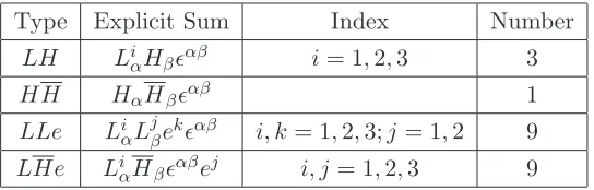
In the present work we restrict our attention to the fields that constitute the electroweak sector of the MSSM. In this particular section that will mean the fields Liα, ei, Hα, and Hα: the lepton doublet and singlet charged lepton, the up-type Higgs doublet, and the down-type Higgs doublet, respectively. The lepton and the electron have a flavor index i= 1,2,3. As they transform as doublets of SU(2), the lepton doublet and the up-type and down-type Higgs fields carry an SU(2) index α = 1,2. All other MSSM matter fields are endowed with a color index and thus have vanishing vacuum expectation values. For now, we do not include the right handed neutrinosνi, which are uncharged under the Standard

3

JHEP03(2016)079

Type Explicit Sum Index Number

LH Li

αHβǫαβ i= 1,2,3 3

HH HαHβǫαβ 1

LLe LiαL j βe

k_ǫαβ _{i, k = 1,2,3;j= 1,2 9}

LHe Li

αHβǫαβej i, j= 1,2,3 9

Table 1. Generators of the GIOs for the electroweak sector of the MSSM.

Model gauge group. As such, we have 13 component fields in the electroweak sector, which means that there is a priori as many F-term equations arising from derivatives of the superpotential. A minimal list of generators for the GIOs of the MSSM electroweak sector is given in table1.

Since the vacuum geometry lives in the image of the ring map (1.5), the F-term con-straints impose restrictions on the ideal of relations among the GIOs. These concon-straints have two effects:

i. they might simply lift some GIOs from the vacuum, by forcing these GIOs to have vanishing expectation values;

ii. they might introduce extra internal relations among the GIOs.

The geometry, or geometries plural, defined solely by the GIOs corresponds to the ideal of their relations, or syzygies.4 Such geometries serve, in some sense, as master spaces common to many of the outcomes we will study in this paper. These geometries may be thought of as the vacuum moduli spaces given by the non-vanishing GIOs when the F-term equations do not impose additional relations among themselves. This is the case when the effect of F-term equations is simply to lift some of the GIOs (outcome i. above). It is therefore important to understand what are the possible varieties arising in this way. First, let us consider the simplest cases. We begin with the set S = {LH, HH}, which consists of four objects (note that we are suppressing the generation indices in our notation). We observe that these are freely generated: there are no relations among the generators. The geometry described is thus trivial and corresponds to C4_{. This holds as} well for any subset of these operators, in which case the geometry is given byCn_{, wheren} is the number of elements in S.

The next-simplest case is the first for which non-trivial relations arise. We consider the nine objects defined by the set {LLe} or the nine objects defined by the set {LHe}. Both of these types of generators can be written as a product of two SU(2) singlets with opposite hypercharges:

χi₁χj₋₁ with i, j = 1, . . .3, (2.1) whereχ−1 stands for the electrone(hypercharge +1) andχ1is eitherLLorLH(both with

hypercharge −1). It is straightforward to realize that, considering each type individually,

4

JHEP03(2016)079

these GIOs are subject to relations,

(χi₁χj₋₁)(χk₁χl₋₁) = (χi₁χl₋₁)(χk₁χj₋₁). (2.2) These equations define the Segre embedding of P2 _×P2 _into P8_{, where} Pn _{is the n} -dimensional complex projective space. Indeed, each of the three χ±1 gives rise to a

coor-dinate in P2_{. The operator LL is described by a Grassmannian Gr(3,2) =}P2 _{due to the} antisymmetrization of the indices, and LH and e both have a free index running from 1 to 3 and therefore corresponds to aP2 _{upon projectivization. The embedding therefore is} the following. Take [x0 :x1 :x2] and [z0 :z1 :z2] as the homogeneous coordinates of two

P2_{s and consider the quadratic map}

LLorLH e LLeorLHe

P2 _× P2 _−→ P8

[x0:x1:x2] [z0 :z1:z2] 7→ xizj

, (2.3)

wherei, j= 0,1,2, giving precisely 32 _{= 9 homogeneous coordinates ofP}8_{. We can}

summa-rize this space with the standard notation (8|5,6|29), where (k|d, δ|mn1₁ mn2₂ . . .) means an affine variety of complex dimensiond, realized as an affine cone over a projective variety of dimensiond−1 and degreeδ, given as the intersection ofni polynomials of degreemi inPk. The Segre embedding is a Severi variety and its corresponding Hilbert series of the first kind is

1 + 4t+t2

(1−t)5 . (2.4)

Since the numerator has coefficients that are palindromic, the space is an affine Calabi-Yau manifold, in the sense that it has a trivial canonical sheaf.5 _{The exponent in the}

denominator gives the dimension of the variety.

One important point to emphasize is the fact that LLeandLHegive rise to the same varieties. This stems from the fact that we have threeLLcombinations as well as threeLH combinations. This coincidence is due to the number of particle generations and Higgses. From the anti-symmetrization of the SU(2) indices in LL, there are only three possible combinations: 3₂ = 3. The LL therefore yields a Grassmannian Gr(3,2), but we have Gr(3,2) =P2_{. On the other hand, the flavor index is free on LH, but, as the Higgs field} bears no index, there are also only three LH. The “symmetry” between LLe and LHe thus only holds for three generations of matter fields and one generation of Higgs fields. Thus far, vacua based solely on relations amongst GIOs fail to distinguish between leptons and Higgs fields.

Let us now consider the two sets togetherS′ _{={LLe, LHe}. Extra relations among the}

18 objects in this set will now appear due to the fact that both types share common fields. With the help of Macaulay 2, we find that these relations describe a seven-dimensional variety given by 51 quadratics (17|7,30|251). The Hilbert series obtained is

1 + 11t+ 15t2_{+ 3t}3

(1−t)7 . (2.5)

5

JHEP03(2016)079

Thus, because the numerator does not have palindromic coefficients, the geometry is no longer Calabi-Yau.

We can understand this variety in the following manner. SinceLandH bear the same quantum numbers, they are not distinguishable from a gauge theory standpoint. Each GIO in the set S′ is thus a product χ1χ−1, where χ−1 are the electron e and χ1 are the

4 2

= 6 possible field configurations φαφβǫαβ with φ ∈ {L, H}. This corresponds to the Grassmannian Gr(4,2). Therefore, we have the following embedding originating from the relations (2.2):

{LL, LH} e {LLe, LHe}

Gr(4,2) × P2 _−→ P17

[x0 :x1 :x2:x3:x4:x5] [z0 :z1:z2] 7→ xizj

, (2.6)

wherexi are Pl¨ucker coordinates subject to the relation,

x0x5 =x1x4−x2x3. (2.7)

The dimension of Gr(4,2) is four, as we have dim Gr(n, r) =r(n−r). Therefore, with the three additional electron coordinates, we obtain a seven dimensional variety as required.

Finally, we should compute the geometry when all possible generators of table 1 are considered together, S′′ _{= {LLe, LHe, LH, HH}. We obtain an irreducible nine}

dimen-sional variety given by 63 quadratic relations: (21|9,56|263_{). The Hilbert series is}

1 + 13t+ 28t2+ 13t3+t4

(1−t)9 . (2.8)

Remarkably, the variety is a Calabi-Yau again. This of course corresponds to the vacuum geometry for the MSSM electroweak theory when there is no superpotential: W = 0.

The geometry can be explained in the following way. The set of ten operators

{LL, LH, LH, HH}, (2.9)

describes a Grassmannian Gr(5,2) from the antisymmetrized product of the SU(2) indices. This is a six dimensional variety. The three electron fields give three additional dimensions and the resulting total variety is therefore nine dimensional:

{LL, LH, LH, HH} e {LLe, LHe, LH, HH}

Gr(5,2) × P2 _−→ C22

[x0 :x1:x2:x3:x4:x5 :x6 :x7 :x8 :x9] [z0:z1 :z2] → (xizj, x6, x7, x8, x9)

,

(2.10) where i= 0, . . .5 and j = 0, . . .2 and the Grassmannian coordinatesx are subject to the relations:

x0x5+x2x3−x1x4 = 0,

x0x8+x2x6−x1x7 = 0,

x0x9+x4x6−x3x7 = 0,

x1x9+x5x6−x3x8 = 0,

JHEP03(2016)079

In (2.10), thex0, . . . , x5 variables corresponding to {LL, LH}are contracted with an

elec-tron field zj, while the remaining four variables x6, . . . , x9 correspond to the hypercharge

neutral operators {LH, HH}. In this case the embedding space is not a projective space. We are now ready to understand the effects of F-term equations on the vacuum geom-etry resulting from the sets of GIOs considered. This is developed in the next section.

3 F-terms constraints

In addition to the syzygies of the GIOs, the vacuum geometry is governed by the constraints arising from F-term equations. The most general superpotential consistent with R-parity at the renormalisable level that can be written with GIOs of table1 corresponds to

Wminimal=C0

X

α,β

HαHβǫαβ+ X

i,j

C_ij3eiX α,β

Lj_αHβǫαβ, (3.1)

where C0 and C3 are coupling constants. This is the electroweak superpotential of the MSSM (without neutrinos). The imposition of R-parity, in the present context, amounts to requiring that each term inW contain an even number of multiplets which carry lepton number. In search of a selection mechanism based on geometrical principles, we would like to understand what, if anything, is special about the above superpotential from the per-spective of vacuum geometry. For this we will investigate deformations to (3.1), considering combinations of the electroweak GIOs, without necessarily insisting on conserved R-parity. We can then compare the corresponding vacuum geometry for each superpotential.

In the absence of right-handed neutrinos, the allowed supertpotential terms are also the GIOs listed in table 1. They can be grouped naturally into two categories. First, we consider the set,

T =LHe, LLe , (3.2)

which we will refer to aselemental trilinears. This terminology comes from the fact that they are the product of three fields (trilinear) that do not constitute a product of other GIOs. Thus they are elemental, as opposite to composite. In addition to these trilinears, we need to consider the elemental bilinears,

B=HH, LH . (3.3)

Again, they are products of two fields which are not GIOs themselves, hence the name elemental bilinears.

JHEP03(2016)079

W terms Vacuum moduli space

LLe+LHe LH HH dim geometry operators

X ₄ C4 _{LH, HH}

X X _{0 point at the origin –}

X X _{0 point at the origin –}

X X X _{0 point at the origin –}

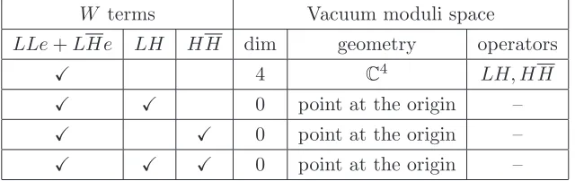
Table 2. Vacuum moduli space for superpotentials W including two elemental trilinears. The dimension (dim), a description of the geometry, and which operators are non-vanishing in the vacuum are presented against the GIOs present in the superpotential (marked with a tick).

3.1 Cases with two elemental trilinears

The first thing to note is that non-trivial geometry can only arise from relations between the LLe and/or LHe operators, as described in section 2. Including either term in the superpotential lifts the corresponding GIO. This is clear from the requirement that the F-term expressions arising from the singlet lepton vanish in the vacuum: ∂W/∂ei _{= 0.} Thus, inclusion of both trilinears simultaneously in the superpotential can only lead to a trivial geometry (consisting of points or planes). When W = LLe+LHe the vacuum is determined exclusively by the GIOs in the set S ={LH, HH}, so the vacuum geometry isC4_{. Further adding elemental bilinears from (3.3) introduces the up-type Higgs fieldH,} whose F-term equation immediately lifts the bilinear GIOs from the vacuum as well. The four possible combinations of superpotentials are summarized in table 2.

3.2 Cases without any elemental trilinear

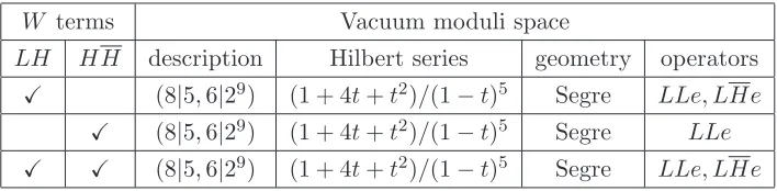
When considering superpotentials without any trilinear, we obtain the Segre variety as the vacuum geometry for all three combinations of LH and HH. Indeed, it is not possible to lift LLeorLHewithLH andHH terms only. The LH andHH GIOs are lifted from the vacuum either by the FL-term and/or the F_H-term equations, both of which impose the vanishing of theH-field in the vacuum for the three superpotential cases.

JHEP03(2016)079

W terms Vacuum moduli space

LH HH description Hilbert series geometry operators

X _(8|5,6|29_{) (1 + 4t+t}2_)/(1−t)5 _{Segre LLe, LHe} X _(8|5,6|29_{) (1 + 4t+t}2_)/(1−t)5 _{Segre LLe} X X _(8|5,6|29_{) (1 + 4t+t}2_)/(1−t)5 _{Segre LLe, LHe}

Table 3. Vacuum moduli space for superpotentialsW without any elemental trilinear. The descrip-tion according to our standard notadescrip-tion, the Hilbert series, the geometry, and which operators are non-vanishing in the vacuum are presented against the GIOs present in the superpotential (marked with a tick).

the vacuum geometry. We will revisit this circumstance in the presence of right-handed neutrino fields in section4. The three cases are summarised in table 3.

3.3 Cases with only one elemental trilinear

Let us now turn to the more complicated cases of superpotentials with one, and only one, trilinear fromT. We can easily observe that the trilinear present in the superpotential will be lifted from the vacuum due to the Fe-term equation. However, the geometry will be different for the two possible sets of superpotentials, and it is convenient to develop each case separately.

3.3.1 LH e

Let us start with only one term — the LHeelemental trilinear — in the superpotential:

W =C_ij3 Li_αHβǫαβej. (3.4)

Assuming a non-singular C3

ij coefficient matrix, it immediately follows from the Fe-term equations that LH, and henceLHe, must vanish. We also have threeL-term equations,

Hβǫαβej = 0, (3.5)

where we have used the inverse of the coefficient matrix C_ij3. These constraints imply HHei _{= 0, which has two kind of solutions. Either e}i _{6= 0, which implies HH = 0, or} ei _{= 0, which implies that LLe = 0 and HH is unconstrained. In this latter case, LH} is also unconstrained, and we have a copy of C4 _{given by {LH, HH}. The full vacuum} geometry thus consists of two branches, a trivial branch C4_{, and another non-trivial one} including the operators LLeand LH.

The variety described by the ideal of relations among the LLe and LH operators are given by the following embedding,

{LL, LH} e {LLe, LH, HH}

Gr(4,2) × P2 _−→ C13

[x0 :x1 :x2 :x3 :x4 :x5] [z0 :z1 :z2] → (xizj, x3, x4, x5)

JHEP03(2016)079

where i = 0, . . .2 and j = 0, . . .2 and the Grassmann coordinates xi are subject to the Pl¨ucker relation

x0x5 =x1x4−x2x3. (3.7)

We still have one condition left to satisfy from the F-term equation arising from the H-field

C_ij3 Li_αǫαβej = 0. (3.8)

Since the two indicesi, jare contracted, we cannot invert the coefficient matrix to simplify the equations. However, we can redefine the ei _{variables as}

˜

ei≡Cijej. (3.9)

Contracting (3.8) withLk_β we obtain a set of three equations

L1_β(˜e2L2αǫαβ+ ˜e3L3αǫαβ) = 0, L2_β(˜e1L1αǫαβ+ ˜e3L3αǫαβ) = 0,

L3_β(˜e1L1αǫαβ+ ˜e2L2αǫαβ) = 0. (3.10) This suggests that the embedding variablesziin (3.6) can be redefined in a related manner, such that the above conditions reduce to

xi= ˜zi, (3.11)

fori= 0. . .2. This coordinate redefinition and identification was explored in greater detail in previous work [3,4]. In the absence of the extrax3, . . . x5 variables (the LH GIOs) this

would lead to the Veronese embedding ofP2 _intoP5_{. Instead, we here obtain:}

{LL∼e, LH}˜ {LL˜e, LH, HH}

Gr(4,2) −→ C10

[x0:x1:x2:x3:x4 :x5] → (xixj, x3, x4, x5, x6)

, (3.12)

wherei, j= 0, . . .2 andi≤jby symmetry. The notationLLe∼eindicates that here they are not independent degrees of freedom because there is a linear relation between them; we will use this notation henceforth. This embedding gives in fact the same Hilbert series as the Segre embedding and we will refer this vacuum moduli space for the superpotential (3.4) as Segre ∪C4_.

Let us now consider deformations of the superpotential by includingLH. These extra GIOs modify the FL-term equations and introduce FH-term equations. The effect of the FL-term equations is to liftLH andHH. Indeed, we have,

C_ij3 Hβǫαβej+CiHβǫαβ = 0. (3.13)

Contracting back withLk

αimplies thatLH= 0, since the first term vanishes upon contrac-tion by virtue of LH = 0 from the Fe-term equation. Similarly, contracting with Hα, we obtain HH= 0 as the first term vanishes from antisymmetrisation of theα and β indices. Moreover, the new constraintFHβ = 0, contracted back withL

j α, gives

JHEP03(2016)079

W terms Vacuum moduli space

LHe LH HH description Hilbert series geometry operators

X _(8|5,6|29₎† _{(1 + 4t+t}2_)/(1−t)5† _{Segre ∪}C4 _{LLe, LH, HH}

X X trivial trivial C _LLe

X X _(8|5,6|29_{) (1 + 4t+t}2_)/(1−t)5 _{Segre LLe, LH}

X X X trivial trivial C _LLe

† _{Segre branch only.}

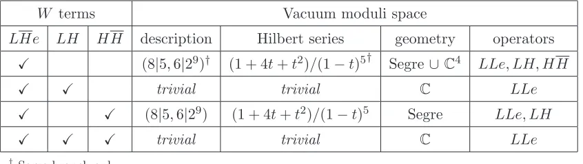
Table 4. Vacuum moduli space for superpotentials W with LHe elemental trilinear. The de-scription according to our standard notation, the Hilbert series, geometry, and which operators are non-vanishing in the vacuum are presented against the GIOs present in the superpotential (marked with a tick).

This holds for the case whenHH is present in the superpotential and when it is not, since any additional terms in FHβ = 0 involving H vanish upon contraction withLby virtue of theFe-term equations, as mentioned earlier. The conditions in (3.14) imply that only one LLeGIO is free, and the geometry becomes a trivial lineC _{with all other GIOs lifted.}

The last case to consider is the superpotential with LHe and HH. It corresponds to the MSSM and the vacuum geometry corresponds to the Segre variety. This has been discussed in great detail in [3, 4]. The vacuum geometries encountered with the LHe trilinear can thus be summarised as in table4.

3.3.2 LLe

Comparing cases with superpotentials containingLLeinstead of LHe, we notice a couple of differences. As before, we start by considering the elemental trilinear only,

W =CijkLiαL j βǫ

αβ_ek_{, (3.15)}

where the coupling coefficients Cijk can be considered antisymmetric in the i, j indices due to the ǫαβ factor. Therefore, the e-term equations will impose the following linear constraints on theLL operators,

  

C121 C131 C231

C122 C132 C232

C123 C133 C233

  ·

  

L1

αL2βǫαβ L1

αL3βǫαβ L2

αL3βǫαβ  

= 0. (3.16)

With generic coefficients, the coefficient matrix will be non-singular. Hence, LL must vanish implying that LLe = 0 in the vacuum. This is somewhat similar to the vanishing of LH in the previous case. However, there is a major difference intrinsic to the relations among GIOs which will lead to a different vacuum geometry.

The non-vanishing GIOs are organised in the following way:

LH e {LH, HH} LHe {LH, HH}

P2 _× P2 _× C4 _−→ P8 _× C4

[x0 :x1 :x2] [z0 :z1 :z2] (x3, x4, x5, x6) → xizj (x3, x4, x5, x6)

JHEP03(2016)079

where i, j = 0, . . . ,2. The fundamental difference with the previous LHe case is that no intrinsic relations exist between LHe and LH as was the case for LLe and LH. The embedding (3.17) simply corresponds to the variety Segre×C4_{, as can be seen from direct} comparison with (2.3).

Turning to the effect of the other F-term equations, we have from theLi

α-term equation,

CijkLj_βǫαβek= 0. (3.18)

Since the coupling coefficients are antisymmetric in i and j we can redefine the electric fields, via a rotation in the field space in the following way,

   ˜ e1 ˜ e2 ˜ e3   =   

C121 C122 C123

C131 C132 C133

C231 C232 C233

  ·    e1 e2 e3  

 . (3.19)

Thus, contracting the conditions (3.18) withHβ, we obtain

L2αHβǫαβe˜1+L3αHβǫαβ˜e2 = 0 L1_αHβǫαβe˜1−L3αHβǫαβ˜e3 = 0

−L1αHβǫαβe˜2−L2αHβǫαβ˜e3 = 0. (3.20)

These equations are similar to the LHe˜case (3.3.1). With an adequate choice of labeling we again havexi= ˜zi and the embedding (3.17) becomes,

LH ∼e˜ {LH, HH} LHe˜ {LH, HH}

P2 _× C4 _−→ P5 _× C4

[x0:x1 :x2] (x3, x4, x5, x6) → xixj (x3, x4, x5, x6)

, (3.21)

where i, j = 0, . . . ,2 and i ≤ j. However, we still have an additional constraint relating LH andLH. Indeed, we can contract (3.18) withHαand multiply withLH. This leads to a set of relations involving LH andLH˜e. In fact, we will obtain the same set of relations linkingx0, x1, x2 with ˜z0,z˜1,z˜2 for the set of variables x3, x4, x5. Thus we have xi+3 ∼xi and x3, x4, x5 can be represented by a factor of proportionality λ. The vacuum geometry

for this superpotential is thus described by,

LH ∼˜e LH HH {LHe, LH}˜ HH

P2 _× C _× C _−→ C9 _× C

[x0:x1:x2] λ x6 → (xixj, λxi) (x6)

. (3.22)

The Hilbert series corresponding to the {LHe, LH}˜ part of the embedding (ignoring x6)

is given by,

(1 + 5t+t2₎

(1−t)4 . (3.23)

JHEP03(2016)079

Let us now consider deformation of the superpotential involving elemental bilinears. First, we should observe that incorporatingHH will trivialise the vacuum. Effectively, the F_H-term equations imply that H = 0 and, thus, LH = HH = 0 in the vacuum. From the FH-term equations, we have two cases depending on whether we include LH in the superpotential or not. If we do not include it, we simply have H = 0 and thusLHe= 0, giving a trivial vacuum where all GIOs vanish. If we do includeLH in the superpotential, we obtain,

C_i′Li_αǫαβ +C0Hαǫαβ = 0, (3.24)

where C_i′ are the coupling constants of theLH operators. Contracting this with Lj_β, and remembering that the LL combinations must vanish from the Fe-term equations, we can conclude that LH= 0. Thus we again have a trivial vacuum where all GIOs vanish.

Finally, we still need to consider the last case of a superpotential with LLeand LH,

W =CijkLiαL j βǫ

αβ_ek_+C′

iLiαHβǫαβ. (3.25)

Again, theFe-term equations imply thatLLemust vanish. The FH-term equation implies that C_i′Li

α = 0. Redefining the L variables by absorbing the coupling constants Ci′, we obtain

˜

L1_α+ ˜L2_α+ ˜L3_α= 0. (3.26)

Moreover, the F_Li

α-term equation leads to

CijkLjβǫ

αβ_ek_+C′

iHβǫαβ = 0. (3.27)

Contracting with Ll

α, and knowing that LLe= 0, we can conclude thatLH = 0.

Equation (3.27) gives us a second relation amongst the GIOs, upon contraction with Hα. For clarity of presentation, we can again absorb the coefficients Ci′ into the lepton doublets ˜Li

α, and redefine the singlet leptons in the same manner as was done in (3.19) previously, to obtain

−L˜2_αHβǫαβe˜1−L˜α3Hβǫαβe˜2=HαHβǫαβ (3.28) ˜

L1_αHβǫαβe˜1−L˜3αHβǫαβe˜3=HαHβǫαβ (3.29) ˜

L1_αHβǫαβe˜2+ ˜L2αHβǫαβe˜3=HαHβǫαβ. (3.30)

We thus have three equations for seven variables (˜e, ˜LH, andHH). They can be interpreted as providing some linear embedding for the HH degree of freedom, which is consequently irrelevant for the geometry. Moreover, only four degrees of freedom remains from theLHe operators. To see this, one may take the difference of equations (3.30) and (3.29), and use the sum rule in (3.26) to arrive at the constraint

−L˜1αHβǫαβe˜1+ ˜L1αHβǫαβe˜2−L˜1αHβǫαβe˜3 = 0. (3.31)

The other combinations arising from (3.28)–(3.30) simply lead to the same constraint equa-tion with ˜L1 _↔L˜2 _↔L˜3 _{interchanged. In the language of the embedding (3.17), the}

JHEP03(2016)079

W terms Vacuum moduli space

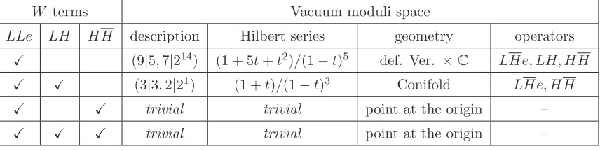
LLe LH HH description Hilbert series geometry operators

X _(9|5,7|214_{) (1 + 5t+t}2_)/(1−t)5 _{def. Ver. ×}C _{LHe, LH, HH} X X _(3|3,2|21_{) (1 +t)/(1−t)}3 _{Conifold LHe, HH} X X trivial trivial point at the origin –

X X X trivial trivial point at the origin –

Table 5. Vacuum moduli space for superpotentialsWwithLLeelemental trilinear. The description according to our standard notation, the Hilbert series, geometry, and which operators are non-vanishing in the vacuum are presented against the GIOs present in the superpotential (marked with a tick).

choice of labeling ˜xi = ˜LiαHβǫαβ and ˜zi=±e˜i, we have,

˜

z0+ ˜z1+ ˜z2 = 0,

˜

x0+ ˜x1+ ˜x2 = 0. (3.32)

Thus, the geometry is described from the following embedding (eliminating the irrelevant HH variables),

˜

LH e˜ LH˜ ˜e

P2 _× P2 _−→ P8

[˜x0 : ˜x1 : ˜x2] [˜z0 : ˜z1 : ˜z2] → x˜iz˜j

, (3.33)

where the ˜x and ˜z are subject to the same relations as above. It turns out that this geometry corresponds to a conifold, and its Hilbert series is given by

(1 +t)

(1−t)3. (3.34)

JHEP03(2016)079

4 Right-handed neutrinos

We now consider how F-term constraints are modified when three generations of right-handed neutrinos are included in the theory. From the standpoint of the MSSM electroweak sector, a neutrino is an absolute singlet, with no charges under SU(2)L×U(1)Y. This makes it unique among the fields we consider, in that it is itself a GIO. It also means that a so-called Majorana mass termW ∋ν2_{is allowed by the gauge symmetries we are considering.}

The sterility of the neutrino under the MSSM gauge group (and its SU(5) GUT ex-tension) is simply a fact. But if the MSSM were to descend from a string construction through an intermediary stage of SO(10) or E6, then we would certainly not expect the

neutrino to be an overall gauge singlet, and ν would not be part of the set of GIOs that establish the vacuum moduli space. Of course, in the case of SO(10) there is a built in matter parity in the form of a gauged U(1)B−L, and neutrinos are clearly identified as leptons. But in the present context the lepton number assignment of the neutrino remains ambiguous: in this case, callingν a “neutrino” field presumes a Yukawa interaction ofLHν in the superpotential. In the present work we hope to understand how singlet extensions of the MSSM with a right handed-neutrino alter the geometrical classification arrived at in the previous section.

Working only at the renormalizable level, the superpotential combinations we consider can contain the standard Dirac mass term built from theLH bilinear, as well as a trilinear coupling built from the HH bilinear. That is, the superpotential couplings can now be enlarged to include the following composite trilinears:

Tν =HHν, LHν , (4.1)

whereν are the right-handed neutrino fields. In principle we could consider superpotential terms linear, quadratic and cubic in the presumed singlet neutrino. In practice, we elimi-nate the tadpole-like linear term, as any such term is unlikely to arise in the superpotential from a fundamental, UV-complete theory. We will also not explicitly include the cubic ν3 term, restricting ourselves to only the putative Majorana mass term,

M =ν2 (4.2)

in our superpotential. More explicitly, any superpotential containing one or more operators from the set

M′ =ν2, ν3 (4.3)

will yield the same vacuum geometry. Thus including the ν3 as an explicit term in the superpotential is redundant.

JHEP03(2016)079

mass term as in (4.2), considering this perturbation only at the end. We then proceed by again splitting the cases according to the number of elemental trilinears present in the superpotential.

4.1 Cases with two elemental trilinears

The first thing to note is that any superpotential with two elemental trilinearsLLe+LHe again lead to trivial vacuum geometries, in the sense that it is composed of points and/or lines. Again, the corresponding GIOs LLe and LHe are lifted from the vacuum and the remaining combinations of LH, HH and ν are only present as invariant polynomials that do not have any relations and syzygies among themselves. We thus arrive at a situation analogous to table 2 with the vacuum moduli space of C7 _{for the case without bilinear} deformation. Addition of aLH orHH removes these bilinears, leavingC3_{, parameterized} by the undetermined neutrino fields.

4.2 Cases without any elemental trilinear

The vacuum moduli space for all possible cases without any elemental trilinear are presented in table 6. Due to the composite nature of some of the superpotential terms, as in (4.1), some vacua can be constituted of two non-trivial branches. We can also observe that all branches have palindromic Hilbert series and are thus Calabi-Yau varieties. This was also true before we introduced right-handed neutrinos, as is evident from table3. For the sake of brevity, from this point onward we will only present the numerator coefficients of the Hilbert series, ordered according the degree oft. That is, (a, b, c, . . .) meansa+bt+ct2+. . ., and the numerator always takes the form (1−t)d_{where dis the dimension of the variety.} In the present case, only two geometries occur. First, we find the Segre variety again with the Hilbert series coefficients (1,4,1) in the numerator. These are the cases from table3. The variation in dimension is simply given by Segre×Cn_{, wheren= 1,3 to obtain} the corresponding dimensions. These additional flat directions are given by the three neutrino fieldsνor theHHoperator, for which no relations are possible withLLeorLHe. The other branches are given by the Hilbert series (1,13,28,13,1) which is the same as the ideal of relations among the GIOs LLe, LHe, LH, HH . However, in the neutrino case, we have an eight-dimensional variety constituted of LLe, LHe, ν . We also have a 10-dimensional one which can be decomposed as CY8 ×C2, where CY8 is an

eight-dimensional Calabi-Yau with Hilbert series (1,13,28,13,1) built out of LLe, LHe, LH . The extra C2 _{comes from neutrino flat directions.}

The appearance of this eight-dimensional Calabi-Yau CY8 is remarkable, in so far as

the Hilbert series numerator (1,13,28,13,1) is also that of the nine-dimensional Calabi-Yau CY9 that defined the vacuum moduli space of the MSSM electroweak sector (2.8).

Recall that this was the vacuum manifold defined by relations amongst the GIOs in the set S′′ _{= {LLe, LHe, LH, HH}, when W = 0. The defining polynomials of the CY}

8 are

those of the CY9 intersected with the surface defined by HH = 0. But, for the cases with

JHEP03(2016)079

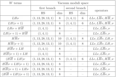
W terms Vacuum moduli space

first branch second branch

operators

HS dim HS dim

LHν (1,13,28,13,1) 8 (1,4,1) 6 LLe, LHe, HH, ν LH(ν+ 1) (1,13,28,13,1) 8 (1,4,1) 6 LLe, LHe, HH, ν

LHν+HH (1,4,1) 8 – – LLe, LHe, ν

LH(ν+ 1) +HH (1,4,1) 8 – – LLe, LHe, ν

HHν (1,13,28,13,1) 10 (1,4,1) 8 LLe, LHe, LH, ν

HH(ν+ 1) (1,13,28,13,1) 10 (1,4,1) 8 LLe, LHe, LH, ν

HHν+LH (1,4,1) 8 – – LLe, LHe, ν

HH(ν+ 1) +LH (1,4,1) 8 – – LLe, LHe, ν

(HH+LH)ν (1,13,28,13,1) 8 (1,4,1) 6 LLe, LHe, HH, ν HHν+LH(ν+ 1) (1,13,28,13,1) 8 – – LLe, LHe, ν

HH(ν+ 1) +LHν (1,13,28,13,1) 8 – – LLe, LHe, ν

(HH+LH)(ν+ 1) (1,13,28,13,1) 8 – – LLe, LHe, ν

Table 6. Vacuum moduli space for superpotentials without any elemental trilinears, including possible bilinear and composite trilinear deformations. The Hilbert series (HS) and dimension (dim) of the different branches of the algebraic varieties are presented in relation to the operators present in the superpotential. The final column lists the type of GIOs that do not vanish in the vacuum. Each of the (1,13,28,13,1) varieties are made out of 63 quadratics and each of the (1,4,1) varieties are made out of 9 quadratics. We would also remind the reader that the degree is easily obtained from the sum of the HS coefficients. Hence the (1,4,1) are of degree 6 and the other ones are of degree 56.

In comparing the various entries in table6, it is clear that in the absence of fundamental trilinears in the superpotential, there is no distinction betweenLandHin terms of vacuum geometry. This is akin to the perfect symmetry in assigning lepton number to the SU(2) doublets that obtained in sections3.1 and 3.2. Another way of stating this finding is that there is nothing geometrically special about the standard Dirac mass term for the neutrino W ∋ LHν in the absence of other fundamental trilinears in the superpotential. Their presence will be the subject of the next subsection.

JHEP03(2016)079

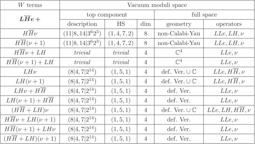
W terms Vacuum moduli space

LH e₊ top component full space

description HS dim geometry operators HHν (11|8,14|3623) (1,4,7,2) 8 non-Calabi-Yau LLe, LH, ν HH(ν+ 1) (11|8,14|3623) (1,4,7,2) 8 non-Calabi-Yau LLe, LH, ν HHν+LH trivial trivial 4 C4 _{LLe, ν}

HH(ν+ 1) +LH trivial trivial 4 C4 _{LLe, ν}

LHν (8|4,7|214) (1,5,1) 4 def.Ver.∪C _{LLe, HH, ν}

LH(ν+ 1) (8|4,7|214) (1,5,1) 4 def.Ver.∪C _{LLe, HH, ν}

LHν+HH (8|4,7|214) (1,5,1) 4 def. Ver. LLe, ν LH(ν+ 1) +HH (8|4,7|214_{) (1,5,1) 4 def. Ver. LLe, ν}

(HH +LH)ν (8|4,7|214_{) (1,5,1) 4 def.Ver.∪C LLe, LH, HH, ν}

HHν+LH(ν+ 1) (8|4,7|214) (1,5,1) 4 def. Ver. LLe, ν HH(ν+ 1) +LHν (8|4,7|214) (1,5,1) 4 def. Ver. LLe, ν (HH+LH)(ν+ 1) (8|4,7|214_{) (1,5,1) 4 def. Ver. LLe, ν}

Table 7. Vacuum moduli space for superpotentials withLHeelemental trilinear, including possible bilinear and composite trilinear deformations. The description, Hilbert series (HS) and dimension (dim) of the top component are presented. The geometry and the type of operators that do not vanish in the vacuum corresponds to the full moduli space.

4.3 Cases with only one elemental trilinear

4.3.1 LH e

Let us consider cases with theLHeoperators first. Results are presented in table7. Again, theFe-term equations lift theLHeoperators from the vacuum in all cases. As with table4, inclusion of the fundamental bilinear LH, alone, will continue to produce a trivial back-ground. But by including the composite trilinearLHν the geometry is altered by relations imposed by the new Fν-term equations. All superpotentials in table7 which contain this Dirac operator for the neutrino result in a deformed Veronese (3.23), independent of other operators that may be present (fundamental bilinears or composite trilinears). But the realization of the deformed Veronese variety in terms of the underlying GIOs is markedly different than in section 3.3.1. In this case, the fieldν takes the role ofLH in the embed-ding, in the same sense that we saw in the previous subsection. Specifically, the embedding is given by:

LL∼e˜ ν {LLe, ν}˜

P2 _× C _−→ C9

[x0 :x1 :x2] λ → (xixj, λxi)

, (4.4)

withi, j= 1,2,3. See [4] for details.

JHEP03(2016)079

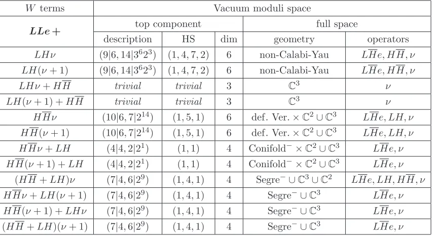
W terms Vacuum moduli space

LLe₊ top component full space

description HS dim geometry operators LHν (9|6,14|36₂3_{) (1,4,7,2) 6 non-Calabi-Yau LHe, HH, ν}

LH(ν+ 1) (9|6,14|3623) (1,4,7,2) 6 non-Calabi-Yau LHe, HH, ν LHν+HH trivial trivial 3 C3 _ν

LH(ν+ 1) +HH trivial trivial 3 C3 _ν

HHν (10|6,7|214_{) (1,5,1) 6 def.Ver.×C}2_∪C3 _{LHe, LH, ν}

HH(ν+ 1) (10|6,7|214_{) (1,5,1) 6 def.Ver.×C}2_∪C3 _{LHe, LH, ν}

HHν+LH (4|4,2|21_{) (1,1) 4 Conifold}−_×C2_∪C3 _{LHe, ν}

HH(ν+ 1) +LH (4|4,2|21_{) (1,1) 4 Conifold}−_×C2_∪C3 _{LHe, ν}

(HH+LH)ν (7|4,6|29_{) (1,4,1) 4 Segre}−_∪C3_∪C2 _{LHe, LH, HH, ν}

HHν+LH(ν+ 1) (7|4,6|29) (1,4,1) 4 Segre−∪C3 _{LHe, ν}

HH(ν+ 1) +LHν (7|4,6|29) (1,4,1) 4 Segre−∪C3 _{LHe, ν}

(HH+LH)(ν+ 1) (7|4,6|29) (1,4,1) 4 Segre−∪C3 _{LHe, ν}

Table 8. Vacuum moduli space for superpotentials withLLeelemental trilinear, including possible bilinear and composite trilinear deformations. The description, Hilbert series (HS) and dimension (dim) of the top component are presented. The geometry and the type of operators that do not vanish in the vacuum corresponds to the full moduli space. The − superscript denotes spaces

analogous to the one indicated, but of one dimension less.

defined by the intersection of three quadratics with six cubic polynomials. This is the only instance in our study in which the variety is defined by a set of cubic relations. The corresponding Hilbert series is

(1 + 4t+ 7t2+ 2t3)

(1−t)8 . (4.5)

The variety is not Calabi-Yau since the Hilbert series is not palindromic.

4.3.2 LLe

Let us now turn to the cases involving the LLe operator. All results are presented in table 8. The LLe GIOs are lifted from the vacuum and we again find a trivial vacuum when including both LLe and HH terms, provided that no HHν terms are present, in complete analogy with the previous case with LHeand LH. We also have the same non-Calabi-Yau variety with Hilbert series coefficients (1,4,7,2) for the case withLHν and no HH operators at all, very similarly to the previous case. However, the dimension of this space is now 6, as opposed to 8. This can be accounted by the fact that the LH operators are being replaced by HH and thus two less degrees of freedom are present.

JHEP03(2016)079

Veronese surface, but instead obtain new vacuum structures. The defining polynomials and Hilbert series data are those of the conifold and the Segre embedding. However, the dimensions are always one less than the usual varieties, despite being described by similar polynomials. That is, we find the Hilbert series (3.34) and (2.4), but with denominators (1−t)2 and (1−t)4, respectively. Therefore, we denote these spaces with the superscript

− _{to differentiate them from the Segre and conifold.}

4.4 Majorana mass term

Thus far, the singlet object denoted by “ν” shows no particular geometric predilection for behaving like the traditional neutrino. The coupling represented by the Yukawa interaction W ∋LHν does not prefer a traditional lepton number assignment for ν. In the absence of fundamental trilinears in the superpotential, both putative lepton number assignments (equivalently, both possible R-parity assignments) yield identical results. This was the principal conclusion drawn from table 6. There is a distinction between, for example, W =LHe+LHν (which gives a deformed Veronese), and W =LLe+LHν (which gives the six-dimensional non-Calabi-Yau geometry). But overall there seems to be nothing about tables7 and 8that suggests a clear lepton number assignment forν.

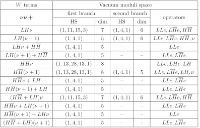
The addition of a quadratic term W ∋ ν2, or Majorana mass term, for the neutrino candidate sharpens the issue considerably. Such a term is commonly invoked to incorporate the see-saw mechanism for neutrino masses, though it is not strictly necessary to explain the neutrino sector of the Standard Model. From the physics point of view, if R-parity is nothing more than a discrete symmetry, here effectively amounting to the rule that all allowed operators must have an even number of “leptons”, then such an operator is consistent with the traditional R-parity assignment when the field ν is designated as a lepton. From the geometrical point of view, including such a Majorana term has the effect of lifting, either partially or completely, the neutrino degrees of freedom from the vacuum manifold. As a result, some of the vacuum structures in tables6through8will change. We will here ask whether these changes tend to favor the cases in which the superpotential is consistent with the traditional R-parity assignments. Our results are presented in table 9 (no fundamental trilinears) and table10 (cases involvingLHeorLLe).

Two kinds of geometries appear which where not present before. In table9, which gives results for superpotentials containing no elemental trilinears, we find the 7-dimensional variety constituted of the relations and syzygies among{LLe, LHe}operators, as presented in (2.6). This is the case for the two superpotentialsW =νν+LHν andW =νν+LHν+ HHν. The remaining vacuum varieties for the case without elemental trilinears are CY8,

Segre and Segre×C_.

JHEP03(2016)079

W terms Vacuum moduli space

ν ν₊ first branch second branch _operators

HS dim HS dim

LHν (1,11,15,3) 7 (1,4,1) 6 LLe, LHe, HH LH(ν+ 1) (1,4,1) 5 (1,4,1) 6 LLe, LHe, HH, ν

LHν+HH (1,4,1) 5 – – LLe

LH(ν+ 1) +HH (1,4,1) 5 – – LLe, LHe

HHν (1,13,28,13,1) 8 – – LLe, LHe, LH HH(ν+ 1) (1,13,28,13,1) 8 (1,4,1) 5 LLe, LHe, LH, ν

HHν+LH (1,4,1) 5 – – LLe, LHe

HH(ν+ 1) +LH (1,4,1) 5 – – LLe, LHe

(HH+LH)ν (1,11,15,3) 7 (1,4,1) 6 LLe, LHe, HH HHν+LH(ν+ 1) (1,4,1) 5 – – LLe, LHe

HH(ν+ 1) +LHν (1,4,1) 5 – – LLe

(HH+LH)(ν+ 1) (1,4,1) 5 – – LLe, LHe

Table 9. Vacuum moduli space for superpotentials including Majorana mass term, without any elemental trilinears. The Hilbert series (HS) and dimension (dim) of the different branches of the algebraic varieties are presented in relation to the GIO types present in the superpotential. The op-erators correspond to the type of opop-erators that do not vanish in the vacuum. Each (1,13,28,13,1) variety is of degree 56 and made out of 63 quadratics. Each (1,4,1) variety is of degree 6 and made out of 9 quadratics. Each (1,11,15,3) variety is of degree 30 and made out of 51 quadratics.

The addition of a Majorana operator ν2 does not trivialize any geometries from ta-bles 6,7 and 8 that were previously non-trivial. In the absence of fundamental trilinears (table6and 9), the impact of adding the Majorana mass term is rather muted, but (signfi-cantly), its impact differentiates between superpotentials involving the lepton doublet and the Higgs doublet, thus breaking the perfect symmetry between these fields seen in table6.

For example, W =LHν and W = HHν both led to the vacuum moduli space CY8

× Segre, in the absence of the Majorana term. Its inclusion deforms the caseW =LHν to the non-Calabi-Yau variety defined by the Hilbert series (2.5) and embedding (2.6), but merely eliminates the Segre component for the caseW =HHν. The caseW =LH(ν+ 1) is deformed even further, from CY8 ×Segre to Segre ×Segre, while only the dimension of

the second Segre factor changes forW =HH(ν+ 1). Thus, in this simple system of super-potentials, the inclusion of a Majorana mass term can distinguish between pairs of cases in whichL↔H, but not every such pair sees a distinction, and the differences are subtle.

JHEP03(2016)079

W terms Vacuum moduli space

LH e₊ν ν₊ top component full space

description HS dim geometry operators LHν (5|3,4|26) (1,3) 3 Veronese ∪C _{LLe, LH, HH, ν}

LH(ν+ 1) (2|2,2|21_{) (1,1) 2 Conifold}−_{∪C∪C LLe, LH, HH, ν}

LHν+HH (5|3,4|26) (1,3) 3 Veronese LLe, LH, ν LH(ν+ 1) +HH (2|2,2|21) (1,1) 2 Conifold−∪C _{LLe, LH, ν}

HHν (8|5,6|29_{) (1,4,1) 5 Segre LLe, LH, HH, ν}

HH(ν+ 1) (8|5,6|29) (1,4,1) 5 Segre ∪C3 _{LLe, LH, HH, ν}

HHν+LH trivial trivial 1 C _LLe

HH(ν+ 1) +LH trivial trivial 1 C _LLe

(HH+LH)ν (5|3,4|26_{) (1,3) 3 Veronese ∪C LLe, LH, HH, ν}

HHν+LH(ν+ 1) (2|2,2|21) (1,1) 2 Conifold−∪C _{LLe, LH, ν}

HH(ν+ 1) +LHν (5|3,4|26_{) (1,3) 3 Veronese LLe, LH, ν}

(HH+LH)(ν+ 1) (2|2,2|21) (1,1) 2 Conifold−∪C _{LLe, LH, ν}

LLe₊ν ν₊ top component full space

description HS dim geometry operators LHν (6|4,4|26_{) (1,3) 4 Veronese×C LHe, HH}

LH(ν+ 1) (3|3,2|21) (1,1) 3 Conifold−×C_∪C2 _{LHe, HH, ν}

LHν+HH trivial trivial 0 point – LH(ν+ 1) +HH trivial trivial 0 point –

HHν (8|4,7|214_{) (1,5,1) 4 def. Ver. LH, LHe}

HH(ν+ 1) (8|4,7|214) (1,5,1) 4 def. Ver.∪point LH, LHe, ν HHν+LH (2|2,2|21_{) (1,1) 2 Conifold}− _LHe

HH(ν+ 1) +LH (2|2,2|21) (1,1) 2 Conifold−∪point LHe, ν (HH+LH)ν (5|3,4|26) (1,3) 3 Veronese ∪C2 _{LHe, HH}

HHν+LH(ν+ 1) (2|2,2|21_{) (1,1) 2 Conifold}− _LHe

HH(ν+ 1) +LHν (2|2,2|21) (1,1) 2 Conifold−∪point LHe, ν (HH+LH)(ν+ 1) (2|2,2|21_{) (1,1) 2 Conifold}−_{∪point LHe, ν}

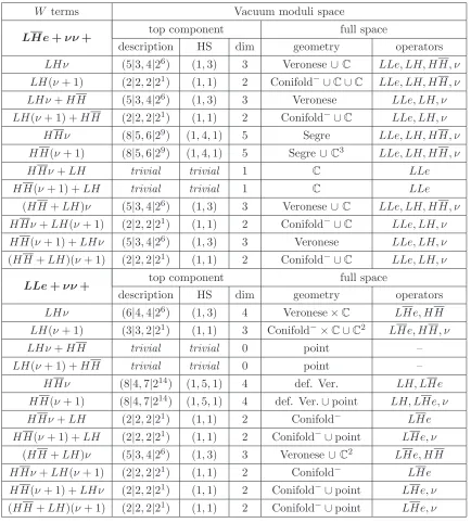
Table 10. Vacuum moduli space for superpotentials with Majorana mass term and one elemental trilinear. The description, Hilbert series (HS) and dimension (dim) of the top component are presented. The geometry and the type of operators that do not vanish in the vacuum corresponds to the full moduli space.

variety arising from cubic relations, with Hilbert series (4.5), is deformed to the previously analyzed Segre variety for W = LHe+HHν +ν2 _{and W = LHe+HH(ν + 1) +ν}2_,

to the Veronese surface for W =LLe+LHν+ν2, and to the two-dimensional conifold− variety for W = LLe+LH(ν+ 1) +ν2_{. Without the Majorana mass term, all of these}

JHEP03(2016)079

So the addition of the Majorana mass term can produce a distinction between a su-perpotential W and its “R-parity dual” Wf(L ↔ H) when none existed in its absence. It can also make pre-existing distinctions more complex. Let us consider the fate of en-tries 5-8 in table 7. In all of these cases (which include the MSSM EW sector with Dirac neutrino masses) the vacuum geometry is that of the deformed Veronese. All four en-tries change when the Majorana mass term is included. The traditional MSSM-like cases, W = LHe+LHν +ν2 and W = LHe+LHν+ν2 +HH, each become the Veronese surface, while the addition of the R-parity violating term LH reduces the variety to the conifold−_{. The R-parity dual cases fW are the entries 5-8 in table 8. The addition of the}

Majorana mass term has far less impact on these cases, and the Veronese surface never appears in this subset when the elemental trilinear isLLe.

This subset of cases is particularly relevant in that it contains the superpotential for the MSSM electroweak sector with a see-saw mechanism for the right-handed neutrinos. Both the case with and without a bilinear for the Higgs fields produce the Veronese sur-face, whereas inclusion of R-parity violating terms such as LLeand LH would produce a trivial vacuum or a 2D conifold, respectively. Only at this stage in our analysis does some geometrical preference start to emerge for the conventional R-parity-conserving MSSM electroweak sector — the Veronese variety prefers the fundamental trilinear LHe, though the presence of a fundamental Higgs bilinear is not particularly preferred, with its the cases HHν and HH(ν + 1) also producing the Veronese variety. These latter cases leave the lepton-number assignment of the neutrino ambiguous, but continue to forbid fundamental operators such asLH and LLein the superpotential.

5 Discussion and outlook

This paper provides a complete classification of the vacuum geometries of all possible renor-malizable theories built from the fields of the MSSM electroweak sector. This represents the culmination of a research program that began one decade ago [1, 2]. At that time, computational algebraic geometry techniques allowed for a determination of the dimension of the vacuum moduli space, and little else. Today a much richer understanding of these spaces is possible. The non-trivial geometries in a system as simple as the SU(2)L×U(1)Y sector of the MSSM are surprisingly diverse, comprising Severi varieties, Calabi-Yau spaces, conifolds of various dimension, and various deformations on these spaces.

JHEP03(2016)079

The complete classification achieved in this work includes cases for which the standard R-parity is conserved, and those for which some R-parity violation is allowed. In a related vein, it also includes cases for which an unambiguous (conserved) lepton number can be assigned to the right handed neutrino, and cases in which the superpotential would make such an assignment ambiguous, or lead to the non-conservation of this lepton number. We find non-trivial geometries emerge in all of these superpotential categories.

Distinctions between a superpotential W and its R-parity dual Wf, obtained via the transposition L ↔ H, do indeed emerge, even in the absence of right-handed neutrinos, in certain circumstances. We began by studying the vacuum geometries determined by the relations that arise solely among the GIOs of the theory. Intriguingly, the geometries generated by the blilinear portion of the GIOs show precisely zero distinction between the fields Land H. The algebraic variety defined by the relations amongst theLLeGIOs and the LHe GIOs are also identical, but in this case this is an accidental symmetry, made possible by the simple fact that there are three species of L fields, but a single H field in the MSSM.

When we add F-term constraints, we continue to see that no distinction between L and H emerges when the superpotential contains only fundamental, gauge-invariant bilinear terms. Allowing for composite trilinears, in which the singlet field ν is allowed to couple to fundamental bilinears, producing terms likeLHν andHHν, continues to exhibit a fundamental invariance under the R-parity swapL↔H. If the superpotential is further augmented to include a Majorana mass term, then these cases do produce slightly different vacuum geometries, but it would be difficult to argue that any one particular configuration was somehow privileged over the others.

On the other hand, we have clear evidence that the vacuum geometry of the MSSM electroweak sector is not completely silent on the issue of R-parity and lepton number conservation. The most obvious evidence for this is that superpotentials which contain both elemental trilinears,LLe+LHe, always generate trivial vacuum moduli spaces. Thus, geometrical considerations seem to force the model-builder to take sides, between admitting LHeas a fundamental trilinear, orLLe. The presence of these objects in the superpotential always lifts the corresponding GIO from the description of the vacuum moduli space. The difference between the resulting moduli spaces can then be identified in the nature of the syzygies between the trilinear operator with the opposite R-parity assignment and the bilinear GIOs. As these constraints descend from the Fe-term equations (arising from the F-terms associated with the charged lepton superfields), it is reasonable to assume that these lessons carry forward into a treatment of the full MSSM.

JHEP03(2016)079

neutrino mass operator LHν perturbs the vacuum manifold to the deformed Veronese. Severi varieties are only recovered when a Majorana mass term is included as well.

However, the Veronese variety is not unique to the R-parity even fundamental trilinear. Both the caseW =LHe+LHν+ν2andW =LLe+LHν+ν2 give a Veronese surface. We can say that the non-trivial vacuum geometries clearly favor cases driven by the relations amongst the LLe GIOs, and therefore a superpotential where this term is absent. But they are not restricted to these cases. More interesting is the ambiguity about the nature of lepton number assignments. The presence of a fundamental Higgs bilinear HH is not necessary to generate a rich vacuum structure, and superpotentials containing HHν and HH(ν+ 1) are equally capable of producing the Veronese variety.

It seems that the ultimate understanding of the geometrical nature of R-parity con-servation may require a definite answer to the logically prior question of the geometrical implication of a conserved lepton number, carried by the neutrino field ν. In such a world the set of GIOs to consider would change. Vacuum geometries would be different, even in the absence of superpotentials, because the relations between the new GIOs in a theory such as SU(2)L×U(1)Y ×U(1)L would be different. We expect that such relations would be more complex, in that operators neutral under the combined gauge group would need to be larger in mass dimension, suggesting a larger elimination problem to compute. The defining polynomials of the vacuum varieties would likely have larger degree, for example. It would be of great interest to determine whether Severi varieties continue to arise in such circumstances, and whether a clearer preference for R-parity even superpotentials can be inferred.

Acknowledgments

We thank James Gray and Mike Stillman for enjoyable collaborations on related themes. YHH would like to thank the Science and Technology Facilities Council, U.K., for grant ST/J00037X/1, the Chinese Ministry of Education, for a Chang-Jiang Chair Professorship at NanKai University as well as the City of Tian-Jin for a Qian-Ren Scholarship, as well as City University, London and Merton College, Oxford, for their enduring support. VJ is supported by the DST/NRF South African Research Chairs Initiative. CM is grateful to Damien Matti and EPFL for providing computing resources and is indebted to the National Institute for Theoretical Physics, the Mandelstam Institute for Theoretical Physics, and the University of the Witwatersrand for hospitality and financial support. BDN would like to thank the International Centre for Theoretical Physics (ICTP) in Trieste, Italy for hospitality during formative stages of this work. His work is supported by the U.S. National Science Foundation under grant PHY-0757959.