An airborne acoustic method to reconstruct a dynamically rough flow surface

This is a repository copy of An airborne acoustic method to reconstruct a dynamically rough flow surface.

White Rose Research Online URL for this paper: http://eprints.whiterose.ac.uk/105121/

Version: Accepted Version

Article:

Krynkin, A. orcid.org/0000-0002-8495-691X, Horoshenkov, K.V. and Van Renterghem, T. (2016) An airborne acoustic method to reconstruct a dynamically rough flow surface. Journal of the Acoustical Society of America, 140 (3). pp. 2064-2073. ISSN 0001-4966 https://doi.org/10.1121/1.4962559

Reuse

Unless indicated otherwise, fulltext items are protected by copyright with all rights reserved. The copyright exception in section 29 of the Copyright, Designs and Patents Act 1988 allows the making of a single copy solely for the purpose of non-commercial research or private study within the limits of fair dealing. The publisher or other rights-holder may allow further reproduction and re-use of this version - refer to the White Rose Research Online record for this item. Where records identify the publisher as the copyright holder, users can verify any specific terms of use on the publisher’s website.

Takedown

If you consider content in White Rose Research Online to be in breach of UK law, please notify us by

An airborne acoustic method to reconstruct a dynamically rough flow

1

surface

2

Anton Krynkin1

, Kirill V. Horoshenkov

3

Department of Mechanical Engineering, University of Sheffield,

4

Sheffield, S1 3JD, UK

5

Timothy Van Renterghem

6

Department of Information Technology, Ghent University, St.-Pietersnieuwstraat

7

41, 9000 Gent, Belgium

8

Abstract 9

Currently, there is no airborne in-situ method to reconstruct with high 10

fidelity the instantaneous elevation of a dynamically rough surface of a turbu-11

lent flow. This work proposes a new holographic method that reconstructs the 12

elevation of a 1-D rough water surface from airborne acoustic pressure data. 13

This method can be implemented practically using an array of microphones 14

deployed over a dynamically rough surface or using a single microphone which 15

is traversed above the surface at a speed that is much higher than the phase 16

velocity of the roughness pattern. In this work, the theory is validated using 17

synthetic data calculated with the Kirchhoff approximation and a finite dif-18

ference, time domain method over a number of measured surface roughness 19

patterns. The proposed method is able to reconstruct the surface elevation 20

with a sub-millimetre accuracy and over a representatively large area of the 21

surface. Since it has been previously shown that the surface roughness pattern 22

reflects accurately the underlying hydraulic processes in open channel flow (e.g. 23

[Horoshenkov, et al, J. Geoph. Res.,118(3), 18641876 (2013)]), the proposed 24

method paves the way for the development of new non-invasive instrumen-25

tation for flow mapping and characterization that are based on the acoustic 26

holography principle. 27

PACS: 43.20.Ye, 43.30.Hw, 43.28.Gq

28

Keywords: Acoustic scattering, roughness, dynamic surface, inverse method

I

Introduction

30

Understanding the spatial and temporal hydraulic changes in rivers and other types

31

of open channels is of paramount importance for predicting flood risk, sediment

32

movement and consequent morphological change. Understanding the spatial and

33

temporal variability of flows has become a core element in assessing the water quality

34

and ecological status of rivers (EU Water Framework Directive (WFD)). However,

35

there is a significant shortcoming in our ability to monitor these flows at sufficient

36

temporal and spatial resolution particularly during extreme events because there is

37

no technology that can be deployed rapidly to accurately map the hydraulic and

38

topographical information of rivers at a reach scale. Although attempts have been

39

made to measure the dynamic surface roughness pattern underwater (e.g. [1, 2]),

40

there is still a lack of real time airborne methods to measure the instantaneous surface

41

elevation with sub-millimeter accuracy and at a very high temporal resolution. This

42

information is of great importance for us to advance the existing theoretical link

43

between the free surface behaviour and the underlying turbulent flow structures

44

which carry information about the flow and sediment bed [3]. This link can be

45

used to study the changes in the turbulent flow structures and velocity depth profile

46

remotely for a range of open channel flows in the laboratory and in the field using an

47

array of acoustic sensors deployed on a large scale, e.g. with a swarm of unmanned

48

aerial vehicles (UAV).

49

The main focus of this paper is to present a new method based on acoustic

50

boundary integral equations and a pseudo-inverse technique applied to a matrix

51

based equation to recover the instantaneous elevation of a dynamically rough surface

52

at sub-millimeter accuracy, high temporal resolution and a representatively large

53

spatial scale. In particular, this approach enables us to study the acoustic scattering

from an inhomogeneous roughness that supports multiple scales.

55

The paper is organized in the following manner. Section II presents the underlying

56

theory of acoustic scattering. This theory is then used in combination with the matrix

57

inversion method which is described in Section III. Section IV presents the results

58

of the application of the proposed inversion method to the acoustic pressure data

59

which were predicted with the standard Kirchhoff approximation and with the Finite

60

Difference Time Domain (FDTD) method. The conclusions are drawn in Section V.

61

II

Scattering of acoustic waves from a rough

sur-62

face

63

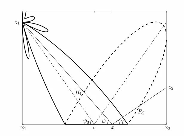
Let us consider a semi-infinite space in Cartesian coordinate system Oxyz bounded

64

by rough surfaceSwhich mean plane S0 coincide withOxycoordinate plane. Spatial 65

scales and distribution of surface elevation ζ(x) are assumed to be arbitrary within

66

the validity range of the proposed method and in this paper both deterministic

67

and random profiles are tested. In order to simplify the numerical calculations, it

68

is assumed that the surface is uniform in Oy-direction and the acoustic source is a

69

directional line source which directivity patternA(x, z) is defined in Section IV. This

70

makes the stated problem one dimensional. The main axis of the far-field directivity

71

pattern is inclined at the angleψ0 with respect to theOxaxis and it is aligned with 72

the centre of coordinates. The coordinates of the source and receiver are defined

73

by (x1, z1) and (x2, z2), respectively. The source emits a continuous harmonic wave 74

exp(₋iωt) with angular frequency ω and constant amplitude in time.

75

In this paper the roughness is defined by the dynamic behaviour of the water flow

76

free surface. To maintain harmonic dependence on time, as suggested above, it is

assumed that the roughness is frozen over a short time period at which the complex

78

acoustic pressure of the scattered harmonic wave needs to be measured. This is true

79

because the speed of sound in air c0 = 340 m/s is much faster than the maximum 80

phase velocityU =U0+cp at which the surface roughness pattern on the flow surface

81

of a typical shallow water river with the mean depth h will propagate, i.e. c0 ≫ U. 82

HereU0 denotes the flow velocity and cp =√gh is the phase velocity of the gravity

83

waves, g is the gravity.

84

In this paper the scattering from a rough surface is approximated by the

tan-85

gent plane approximation as suggested in [4]. We assume that the surface is rigid

86

which is a good approximation for the case when sound propagates in air above a

87

dynamically rough water surface, e.g. free surface of a turbulent open channel flow.

88

The approximation is based on the Kirchhoff method and principles of geometrical

89

optics (e.g. [5]), and it is valid if local curvature radius a of the rough surface is

90

much greater than the acoustic wavelength λ= 2π/k, wherek is wavenumber of the

91

acoustic wave. For the diffraction on a sphere, this condition can be stated in the

92

following form

93

sinψ _≫ 1

(ka)1/3, (1)

whereais a radius of the sphere locally inscribed in rough surface. The condition in

94

eq. (1) can be relaxed to [6]

95

sinψ > 1

(ka)1/3, (2)

so that the Kirchhoff approach remains accurate for the incident angles far from the

96

low grazing angles. In this paper condition (2) is used in the numerical simulation

97

to define the surface.

98

Assuming that the distances from the sourceR1 and receiver R2 to a given point 99

on the mean surface (see Figure 1) are much greater than the acoustic wavelength

0

R1

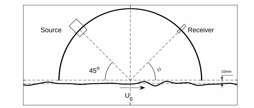
R2

z1

z2

x x2

ψ0 ψ χ

x1

Figure 1: The geometry of the acoustic problem of rough surface scattering.

and using the Kirchhoff method, the scattered acoustic pressure can be approximated

101

by [4, 7]

102

p(x2, z2) =−

i 2πk

Z

S0

A(x)

√

R1R2

exp [ik(R1+R2)−iqzζ(x)]

qz−q ∂ζ(x)

∂x

dx, (3)

whereζ(x) is surface elevation and

qz =k

z1

R1

+ z2 R2

, (4)

q=₋k

x1−x

R1

+ x2 −x R2

, (5)

R1 =

q

(x₋x1) 2

+z2

1, (6)

R2 =

q

(x₋x2) 2

+z2

2. (7)

Assuming that the surface is smooth, ∂ζ(x)/∂x_≪1, equation (3) can be simplified

to

104

p(x2, z2) =−

i 2πk

Z

S0

A(x)

√

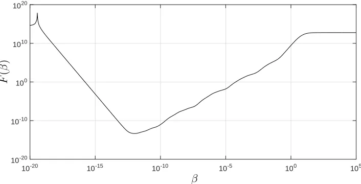
R1R2

exp [ik(R1+R2)−iqzζ(x)]qzdx. (8)

If the profile of the surface ζ(x) is known than the integral in equation (8) can be

105

solved numerically. However, the surface in the above integral is assumed to be

106

unknown and it is the acoustic pressure in the left hand side which is known from

107

experiments or from synthetic data (obtained with the Kirchhoff approximation and

108

FDTD method in this paper). This formulates an inversion problem where the

109

variable ζ(x) needs to be recovered from the available acoustic pressure data.

110

III

Matrix inverse method

111

In order to invert the surface elevationζ(x) it is proposed to use a numerical approach

112

to solve integral equation (8). For this purpose the integral is discretised over the

113

surface S0 with the M uniform spatial elements ∆x = xm+1 − xm, m = 1, ..., M

114

and approximated by the sum over these elements. It is noted that the size of the

115

element ∆x has to be at least five times smaller than the acoustic wavelength λ[6]

116

(i.e. ∆x < λ/5). The scattered acoustic pressure at the receiver position (x2, z2) can 117

be approximated by

118

p(x2, z2) =−

i 2πk

M X

m=1

A(xm) p

R1,mR2,m

exp [ik(R1,m+R2,m)−iqz,mζ(xm)]qz,m∆x, (9)

where all the terms with the index m are defined at points xm, m = 1, ..., M on the

119

surface S0. Equation (9) can be rewritten in the form of a scalar product of two 120

vectors

121

where

D_M =

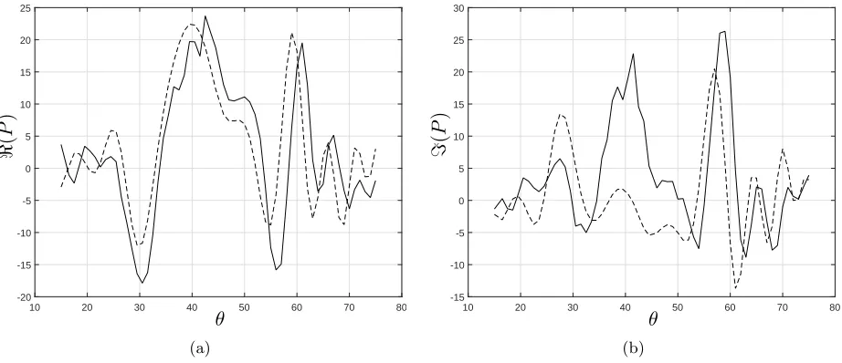
( − i

2πk

A(xm) p

R1_,mR2_,m

exp [ik(R1,m+R2,m)]qz,m∆x )

m=1,...,M

, (11)

E_M =_{exp [₋iqz,mζ(xm)]}_m=1,...,M. (12)

In order to retrieve the surface profile ζ(x) it is necessary to have acoustic pressure

122

data recorded at more than one receiver positions that the acoustic pressure vector

123

P with N elements can be formed. With multiple receiver positions defined by the

124

coordinates (x2,n, z2,n), n = 1, ..., N, equation (10) needs to be converted into the 125

matrix form in order to apply the matrix inversion.

126

One way of deriving the matrix form is to isolate the unknown elevation of the

127

rough surface ζ(x) at the points xm, m = 1, ..., M for all receiver positions in one

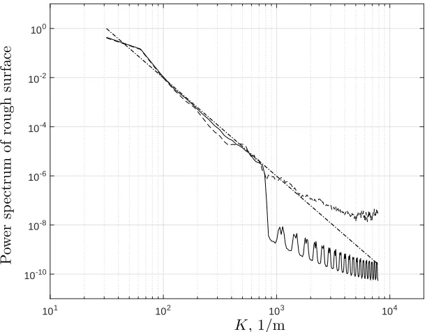
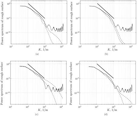
128

single vector E_M. In doing so it is assumed that for fixed index m the variability of

129

qz,mn, n= 1..N with respect to the position on the surface is negligible in the vicinity

130

of the specular point defined by the angle ψ0 as shown in Figure 1. This gives 131

PN×1 =HN×MEM×1, (13)

where the elements of the matrix H_N×M are defined by

132

hmn= (

− i

2πk

A(xmn) p

R1,mnR2,mn

exp [ik(R1,mn +R2,mn)]qz,mn∆x

)

m=1,...,M,n=1,...,N (14)

and unknown vectorEM×1is given by equation (12) withqz,mdefined by the receiver

133

positioned at the specular angle ψ0. The form of equation (13) is identical to that 134

used in inverse frequency response function (IFRF) techniques with HN×M

repre-135

senting transfer matrix for an array of microphones and vector E_M×1 representing 136

velocity potentials on the surface [11]. This allows us to apply previously developed

137

techniques to recover surface profile.

It is practical to assume that the number M of unknown points on the surface is

139

greater than the number of receivers N (M > N). However, this leads to an

under-140

determined system of equations which may result in an ill-conditioned matrix and a

141

non-unique inverse solution to problem stated in equation (13). In order to invert

142

the matrix HN×M in equation (13) it is proposed to use a pseudo-inverse method

143

based on the singular value decomposition technique (SVD) (e.g. [8]). Applied to

144

matrix HN×M this gives

145

HN×M =UN×NSN×MV¯

T

M×M, (15)

where UN×N and VM×M are unitary matrices (defined by AA¯

T

= I), SN×M is

146

a diagonal matrix with nonnegative elements arranged in the descending order of

147

smallness, ¯A stands for complex conjugate and AT denotes matrix transpose. In

148

order to apply pseudo-inverse techniques and decrease the computational time, in

149

this paper the truncated form of matricesS andV in equation (15) was used so that

150

HN×M =UN×NSN×NV¯

T

N×M. (16)

Applying the SVD to equation (13) and using the definition of the unitary matrix

151

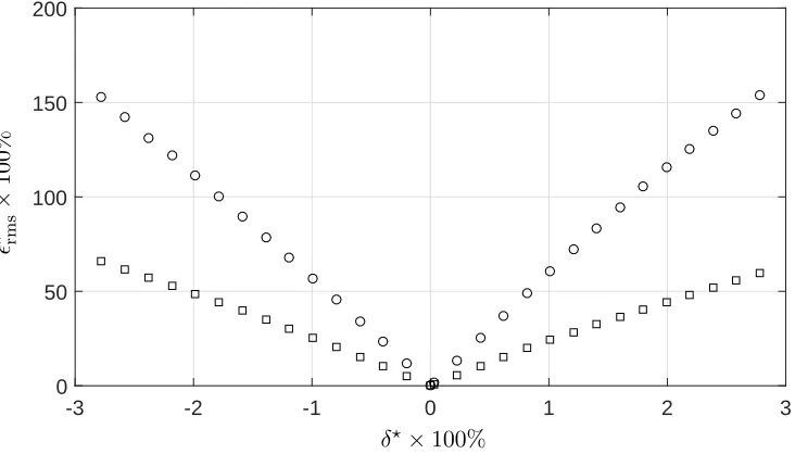
the unknown vector EM×1 can be expressed in the following form 152

EM×1 =VM×NS

−1

N×NU¯

T

N×NPN×1, (17)

where S−1

N×N indicates the matrix inverse. The matrix SN×N may contain small

153

order elements resulting in singular values in the inverted matrixS−1

N×N. In order to

154

regularize ill-conditioned matrix and to filter the singular elements from the inverse

155

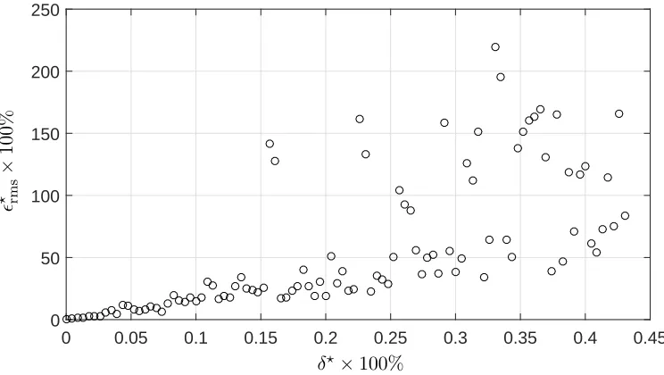
matrix it is proposed to use the Tikhonov regularization technique (e.g. [11] and [9])

156

that gives

157

E_M×1 =VM×NS

−1

β,N×NU¯

T

whereS−1

β,N×N =

SN×N +β

2

S−1

N×N

−1

andβ is the regularization parameter. In

or-158

der to adjust parameterβ we used the generalised cross validation (GCV) technique.

159

This technique requires to minimize the following function

160

F(β) = r

2

β

T rI_N×N −UN×NSN×NS −1

β,N×NU¯

T N×N

2, (19)

in whichrβ is the residue defined by l2-vector norm

161

rβ =

IN×N −UN×NSN×NS

−1

β,N×_NU¯

T N×N

PN×1

. (20)

The argument (phase) of each element of vectorE_M×1provides information about 162

the surface elevation. In order to retrieve the phase from matrix equation (18)

163

the complex natural logarithm is applied element-wise to the results of the matrix

164

product. This yields

165

Qζ_M×1 =−ℑ[Ln(EM×1)], (21)

where

166

Qζ_M×1 ={qz,mζ(xm)}_m=1_,...,M, (22)

with _ℑ(<_·>) representing the imaginary part of the natural logarithm. It is noted

167

that the application of Ln in equation (21) is restricted to the case when ₋π <

168

qz,mζ(xm)< π that enables us to uniquely define the elements of the vector Qζ_M×1. 169

This condition holds in the vicinity of a specular point defined by the angle ψ0 170

and fails as distance between specular point and xm, m = 1, ..., M increases. The

171

discretized roughness profile_{ζm} at the points{xm} can then be deduced as

172

{ζm}m=1,...,M =

−ℑ[Ln(em)] qz,m

m=1,...,M

, (23)

The fact that the proposed inversion largely depends on the proximity of a surface

174

point to the specular point leads to the idea of replacing the directional source with

175

simple monopole with a unit amplitude. As a result, the elements of the matrix

176

H_N×M can be simplified to

177

hmn= (

− i

2πk

exp [ik(R1,mn+R2,mn)]

p

R1,mnR2,mn

qz,mn∆x )

m=1,...,M,n=1,...,N

. (24)

This reduces input data to geometrical parameters defined by the position of source

178

and receivers with respect to the surface S0 and data recorded on the array of re-179

ceivers.

180

IV

Results

181

In this paper, validation of the proposed inversion method (equation (23)) is based on

182

two sets of synthetic data generated using the Kirchhoff integral and FDTD method.

183

The former demonstrates the implementation of the proposed inverse technique and

184

the latter shows application of this technique to independent set of data obtained in

185

order to retrieve unknown surface profile.

186

A

Simulated roughness

187

In this section the acoustic pressure scattered by the rough surface was modelled with

188

the Kirchhoff integral (equation (8)). In order to reconstruct the surface elevation it

189

was proposed to use an array ofN = 121 receivers arranged on a circular arch with the

190

radius ofR = 0.4 m as illustrated in Figure 2. The receivers and source are positioned

191

on the opposite sides of the arch. The arch is suspended at d = 0.01 m above the

192

U 0

10mm

Source Receiver

φ 45o

Figure 2: The acoustic setup used to reconstruct the rough surface in the numerical

experiment.

Ox axis. The source was installed at the angle of ψ0 = 45o and its coordinates were 194

(Rcosψ0, Rsinψ0 +d), where d is the vertical distance of the circular arch base to 195

the planeS0. The position of receivers is defined by (−Rcosφ, Rsinφ+d), where φ 196

varies from 15o _{to 75}o _{with 0.5}o _{resolution that produces 121 receiver positions. The}

197

sound source emitted a continuous harmonic wave at f = 43 kHz and its far-field

198

directivity pattern was defined by

199

A(θ) = J1(kasinθ)

kasinθ , (25)

wherea = 0.02 m is the radius of the source aperture. The position of the receivers

200

was characterized by the angle φ which was taken from the horizontal line. The

201

number of the receivers in the array, N, and the adopted geometry were consistent

202

with that used in the experiments reported by Nichols [10]. Increasing the number

203

of receivers may result in more singular values and it may lead to a more unstable

204

inverse solution. Decreasing the number of the receivers may lead to a poorer spatial

205

resolution of the surface elevation and higher ambiguity.

In the calculations reported in this section the 1-D rough surface ζ(x) was

sim-207

ulated with the Fourier series containing random phase and amplitudes assigned in

208

accordance with the typical characteristics of gravity-capillary waves [12]. This gives

209

ζ(x) =σX n

Cncos (Knx+τn), (26)

where σ is the standard deviation of the rough surface elevation (mean roughness

210

height), Kn is wavenumber in the surface roughness spatial spectrum, τn is phase

211

which value is randomly generated and amplitude Cn is defined by the correlation

212

function of the waves of which the surface roughness pattern is composed and it is

213

proportional to the wavelength ln of the n-th harmonic in the Fourier expansion so

214

that

215

Cn∼

2π ln

α/2

. (27)

In particular the amplitude of each term in the Fourier expansion is linked to the

216

power spectrum slope defined by the power of α = ₋4 [13]. The surface elevation

217

constructed with this kind of spatial spectrum supported multiple scales ranging

218

from 8 mm to 115 mm and satisfied the condition (2) on the validity of Kirchhoff

219

approximation. The standard deviation of the surface is set toσ = 1 mm.

220

Figure 3(a) shows the surface elevation simulated with the Fourier series using

221

the range of spatial wavelengths of 8mm< ln <115 mm and compared with surface

222

elevation reconstructed with the proposed inversion method. This figure also shows

223

the absolute error in the surface reconstruction which was calculated as ǫζ(x) =

224

|ζp(x)−ζs(x)|, whereζp(x) is the surface elevation predicted with the inverse method

225

and ζs(x) is the surface elevation simulated with equation (26). The inversion was

226

applied to the surface interval containingM = 3000 surface points that included the

227

specular reflection point and its vicinity. It can be seen from the data presented in

228

Figure 3 that the range ofxfor which the surface roughness reconstruction could be

x, m

-0.4 -0.3 -0.2 -0.1 0 0.1 0.2 0.3

ζ

(

x

),

m

×10-3

-3 -2 -1 0 1 2 3 4

(a)

(a)

x, m

-0.4 -0.3 -0.2 -0.1 0 0.1 0.2 0.3

ǫζ

(

x

),

m

×10-3

0 1 2 3 4 5 6 7

(b)

(b)

Figure 3: (a) An example of the surface realization, ζ(x), (dashed line) used in

equation (8) and its reconstruction from the Kirchhoff approximation (solid line)

based on equation (23). (b) Absolute error of the reconstructed surface.

achieved was limited by the position of the specular reflection point which was in the

230

range of -0.1 m< x <0.1 m. In particular, this is illustrated in Figure 3(b) where the

231

absolute error of the surface reconstructed within this interval is limited and does not

232

exceed 0.22 mm which is considerably smaller than the maximum roughness height

233

of 2.5 mm. The root mean square (RMS) error for this range does not exceed 0.12

234

mm that is 12% of the true mean roughness height. In this analysis the root mean

235

square error was calculated as

236

ǫrms=

v u u

t1

N N X

n=1

[ζp(xn)₋ζs(xn)]2_{, (28)}

where the deduced surface elevation ζp(xn) and simulated surface elevation ζs(xn)

237

are taken at the point xn. It is noted that these errors are comparable or smaller to

238

those which are typical for an alternative laser-induced fluorescence (LIF) method

10-20 10-15 10-10 10-5 100 105 10-20

10-10 100 1010 1020

β

F

(

β

)

Figure 4: An example of the behaviour of the functionF(β) for the range of 10−20

<

β <105

.

(e.g. _±0.14 mm for the LIF method used in ref. [10]).

240

The regularization parameter β was selected in accordance with equation (19).

241

Figure 4 illustrates the variation of the GCV functionF for the reconstruction process

242

for the surface shown in Figure 3(a). The parameter β is small (β _∼ 10−12

) and

243

defines the threshold below which equation (18) becomes unstable. It increases with

244

the decrease in the number of receivers causing the inversion process to become more

245

unstable.

246

In order to understand the range of scales which can be recovered with equation

247

(18) we compared the power spectrum of the surface roughness for a representative

248

number of realizations obtained by varying randomly phase with the amplitudes

249

of the Fourier expansion (equation (26)). The power spectrum was calculated by

250

applying the Hanning window and Fourier transform to the original and recovered

251

surface elevation data for each of the surface realization. It was then averaged over

252

all the surface realizations. It was found that the average power spectrum converges

101 102 103 104 10-10

10-8 10-6 10-4 10-2 100

K, 1/m

P

ow

er

sp

ec

tr

u

m

of

ro

u

gh

su

rf

ac

e

Figure 5: The normalized power spectrum averaged over 100 surface elevation

re-alizations. Dash-dot line - the spectrum based on equation (27); dashed line - the

inverted spectrum; solid line - the spectrum of the surfaces generated with equation

(26).

to the true mean value to within 1% provided that at least 100 surface realizations

254

were used. The average power spectrum inverted with the proposed method follows

255

the slope α = ₋4 defined by equation (27) for K < 800 1/m (Figure 5). This

256

corresponds to the lowest scale present in the simulated surface roughness wavelength

257

of ln ≈ 8 mm. For the spectrum of larger scales (centimetre scale) when K < 800

258

the agreement between the average spectrum inverted with the proposed technique

259

and that defined by equation (26) was within 15%.

B

Measured roughness

In order to illustrate the application of the inversion method developed in Section III

262

we used the acoustic pressure dataP_N×1calculated with the Kirchhoff approximation 263

and with the full-wave 2-D FDTD method [14] for a range of roughness realizations

264

measured with the light-induced fluorescence method detailed in [10]. In the case of

265

the Kirchhoff approximation the acoustic pressure was calculated as described in the

266

previous section.

267

In the case of the FDTD method the acoustic pressure was computed for a source

268

with directivity pattern defined by (25). This source directivity was simulated by

269

setting up a 33 mm long line array of 49 point sources operated in phase. The

270

frequency of the acoustic wave emitted by the source wasf = 43 kHz. The time and

271

space discretization intervals in the FDTD calculations were 1.03 µs and 0.5 mm,

272

respectively [15].

273

The surface roughness data used in this work were obtained in a hydraulic flume

274

with the method detailed in [10] and these were assumed to be exact in our

calcu-275

lations. The flume had a bed of hexagonally packed spheres with a diameter of 25

276

mm, and was tilted to a slope of S0 = 0.004. The flow was turbulent, uniform and 277

constant velocity was maintained across the length of the measured spatial interval.

278

The surface elevation data was collected for four flow regimes which corresponded to

279

the flow with the 60, 70, 80 and 90 mm of uniform water depth, respectively. These

280

regimes corresponded to the mean flow velocity of 0.43, 0.50, 0.57 and 0.65 m/s,

281

respectively. The arrangement of the receiver positions in the models was identical

282

to that detailed in the previous section for a given realization of ζ(x).

283

In Figure 6 the real and imaginary parts of the angular dependent acoustic

pres-284

sure predicted with the FDTD method is compared against that predicted with the

10 20 30 40 50 60 70 80 -20

-15 -10 -5 0 5 10 15 20 25

θ

ℜ

(

P

)

(a)

10 20 30 40 50 60 70 80

-15 -10 -5 0 5 10 15 20 25 30

θ

ℑ

(

P

)

(b)

Figure 6: The scattered acoustic pressure for a single realization of the rough

sur-face elevation for flow depth 60 mm predicted with FDTD method(solid line) and

Kirchhoff approximation (8) (dashed line). (a) Real part, (b) imaginary part.

Kirchhoff approximation (8). These results correspond to a realistic flow surface

286

roughness realization measured for the 60 mm deep flow regime. The results suggest

287

that the Kirchhoff approximation generally underpredicts the acoustic pressure in

288

comparison to that predicted by the FDTD method. This is particularly

notice-289

able in the case of the imaginary part and for the angles of incidence close to 45o_.

290

These acoustic pressure data were then used with the proposed inversion technique

291

to reconstruct the flow surface roughness.

292

Figures 7 (a)-(d) present the results of the application of the inverse technique

293

to the acoustic pressure data predicted with the Kirchhoff approximation and with

294

the FDTD method for flow surface realizations representing each of the four flow

295

regimes. The inversion results are shown in the range ₋0.1< x <0.1 m where the

296

maximum relative error was within 45% when the acoustic pressure was predicted

with the FDTD method and 20% when the acoustic pressure was predicted with the

298

Kirchhoff approximation. Within this interval the effects of shadowing and multiple

299

scattering are relatively small that enables us to use equation (8) as an accurate

300

approximation to the full-wave FDTD results. In all cases the minimum of β was

301

in the interval [0,1] and its values is listed in Table 1. The accuracy we achieved

302

depended on how far the point on the surface was from the nominal specular reflection

303

point.

304

Figure 8 presents the mean spatial spectra which demonstrate the range of scales

305

of roughness which were recovered through the proposed inversion technique. These

306

spectra were inverted using the acoustic pressure data predicted with the Kirchhoff

307

approximation and with the FDTD method. As it was noted in the previous section

308

IV A, the normalized power spectrum provides information on the contribution of

309

different roughness scales to the pattern of waves observed on the surface. For the

310

four flow regimes considered in this work the recovered surface predicts the actual

311

slope of the power spectrum closely for K < 1000 1/m. However, it is clear that

312

the accuracy of the proposed inversion techniques deteriorates asK approaches 1000

313

1/m that limits the use of the technique to identify the correct range of roughness

314

scales, i.e. those scales which are at a ln < 6.3 mm spatial wavelength. This can

315

be explained by the limitations of the Kirchhoff approximation (equation (8)) as the

316

local radius of curvature increases with the decrease of the surface scales. It is also

317

noted that, although in this paper the coordinates of the receivers are exact, the

318

implementation of the method can be limited by the uncertainties in the receiver

319

positions. The sensitivity of the proposed method is analysed on Appendix A.

320

It is difficult to obtain a useful measure of the error between the measured

spec-321

trum and that reconstructed with the proposed inversion method by comparing these

322

spectra directly. This is because the spectral power shown in Figure 8 varies by 10

-0.1 -0.08 -0.06 -0.04 -0.02 0 0.02 0.04 0.06 0.08 0.1 ×10-3

-1 -0.5 0 0.5 1 1.5 2 2.5 3

x, m

ζ ( x ), m (a)

-0.1 -0.08 -0.06 -0.04 -0.02 0 0.02 0.04 0.06 0.08 0.1

×10-3

-2 -1.5 -1 -0.5 0 0.5 1 1.5

x, m

ζ ( x ), m (b)

-0.1 -0.08 -0.06 -0.04 -0.02 0 0.02 0.04 0.06 0.08 0.1

×10-3

-3 -2 -1 0 1 2 3 4

x, m

ζ ( x ), m (c)

-0.1 -0.08 -0.06 -0.04 -0.02 0 0.02 0.04 0.06 0.08 0.1

×10-3

-1.5 -1 -0.5 0 0.5 1 1.5 2 2.5

x, m

ζ ( x ), m (d)

Figure 7: Examples of the surface elevation ζ(x) for the four flow regimes. Solid

line - measured with the LIF method; dashed line - reconstructed with the sound

pressure data predicted with the FDTD mode; dashed-dot line - reconstructed with

the acoustic pressure data predicted with the Kirchhoff approximation. (a) Flow

101 102 103 104 10-10

10-5 100

K, 1/m

P ow er sp ec tr u m of ro u gh su rf ac e (a)

101 102 103 104

10-10 10-5 100

K, 1/m

P ow er sp ec tr u m of ro u gh su rf ac e (b)

101 102 103 104

10-10 10-5 100

K, 1/m

P ow er sp ec tr u m of ro u gh su rf ac e (c)

101 102 103 104

10-10 10-5 100

K, 1/m

P ow er sp ec tr u m of ro u gh su rf ac e (d)

Figure 8: The normalized power spectrum of rough surface (solid line) compared

against the power spectrum of the reconstructed surface where dashed and

dashed-dot lines represent the use of FDTD and Kirchhoff approximation data, respectively.

Thick solid line represents slope of the reconstructed power spectrum. (a) Flow depth

orders of magnitude over the considered range of wavenumbers. For this purpose

324

all results in Figure 8 are compared against slope of the measured surface which is

325

deduced with the linear regression technique between K > 100 andK < 1000 1/m.

326

The slope of the measured power spectrum for all flow regimes is approximated by

327

α=₋5. A comparison between fitted line with slope₋5 and spectra recovered with

328

the proposed acoustic method suggests that the method provides adequate prediction

329

of the surface power spectrum.

330

V

Conclusion

331

In this paper we demonstrate the derivation of an inversion method based on the

332

Kirchhoff approximation of the boundary integral equation and the application of an

333

inverse technique based on SVD and Tikhonov regularization to an underdetermined

334

system of equations. The surface roughness data we used in our work were simulated

335

surface roughness and surface roughness measured with the LIF method that were

336

assumed to be exact. The proposed inversion method enables us to determine the

337

1-D surface roughness with a maximum RMS error of 45% (FDTD method) and 20%

338

(Kirchhoff approximation), both being sub-millimeter scale errors. This method also

339

enables us to estimate the average spatial power spectrum of the surface roughness for

340

the range of wavenumbers K < 1000 1/m. This corresponds to spatial wavelengths

341

of ln >6.3 mm. For the simulated surface roughness this spectrum converges to its

342

true mean value to within 15% provided that at least 100 realizations are used in

343

the averaging process. The area of the rough surface which can be reconstructed

344

with the proposed acoustic setup and with the reported accuracy is within _±0.1 m

345

range. This range determines the maximum wavelength in the spatial spectrum of

346

surface which can be estimated with the proposed acoustic setup and it is limited

by the wavelength of the incident acoustic waves, by the number and arrangement

348

of the receivers in the microphone array and by the adopted directivity of the sound

349

source. It is shown that the reconstructed surface roughness power spectrum follow

350

a power law characterising the simulated/measured surfaces.

351

The inversion method requires further improvements to increase accuracy for the

352

scales in the centimeter and sub-centimeter range of spatial wavelength. This should

353

involve the use of an extension of Kirchhoff approximation which can account for

354

higher roughness slopes or a more refined 3D numerical model for 2D roughness.

355

The retrieved roughness profiles can be used to find key statistical and spectral

356

characteristics of the water surface. The proposed method can potentially be used

357

together with the acoustic array measurements to accurately retrieve the temporal

358

and spatial profile of the dynamic shallow water flow.

359

Acknowledgments

360

The authors are grateful to Dr. Andrew Nichols (University of Sheffield) for the

361

provision of the LIF data some of which we used for the analysis reported in Section

362

IV B. The authors would like to thank unanimous reviewer of this paper for valuable

363

comments and suggestions.

364

Appendix A: Sensitivity

365

In order to test the sensitivity of the proposed inverse method it is necessary to

simulate some type of geometrical uncertainty. In the case when position of all

receivers are fixed the uncertainty in position is linked to the coordinates of the

-3 -2 -1 0 1 2 3 0

50 100 150 200

δ⋆_×100%

ǫ

⋆ rm

s

×

10

0%

Figure 9: The relative variation in the RMS surface roughness height reconstructed

for a given uncertainty in thex(squares) and z-coordinates (circles) for the receiver

the 1D surface roughness the coordinates of the array frame can be varied alongOz

and Ox axis. Introducing a small perturbation δ = δ⋆_{R, where δ}⋆ _{is dimensionless}

small parameter, to the distances R1 and R2 shown in equations (6) and (7) the

uncertainty along Oxaxis can be defined by

R1 =

q

(x₋x1+δ) 2

+z2

1, (29)

R2 =

q

(x₋x2+δ) 2

+z2

2. (30)

whereas the uncertainty alongOz axis is given by

R1 =

q

(x₋x1) 2

+ (z1+δ)2, (31)

R2 =

q

(x₋x2) 2

+ (z2+δ)2. (32)

In both cases dimensionless parameter δ⋆ _{varies within 3% of frame radius R around}

366

frame initial coordinates. The results are shown in Figure 9 where the uncertainty

367

is introduced in the inversion with the FDTD simulation of acoustic scattering. It is

368

observed that the variation along the Oz axis depicted in circles results in a higher

369

relative deviation in the RMS roughness height defined by

370

ǫ⋆rms(δ

⋆_{) =} q

PN

n=1[ζp(xn, δ⋆)−ζp(xn, δ⋆ = 0)] 2

q

PN

n=1[ζp(xn, δ⋆= 0)] 2

, (33)

within which ζp represents the predicted surface roughness with the inverse method.

371

The root mean square (RMS) roughness hight reconstructed in the [₋0.1,0.1] m

372

spatial interval deviates linearly from the predicted initial (δ = 0) RMS roughness

373

hight as the position of the frame varies within 3% from the initial position. The

374

uncertainty in Ox coordinate of the frame δ⋆ _{×100% = ±1% with respect to its}

375

radius R results in 25% variation in the RMS roughness height. Applying the same

0 0.05 0.1 0.15 0.2 0.25 0.3 0.35 0.4 0.45 0

50 100 150 200 250

δ⋆_×100%

ǫ

⋆ rm

s

×

10

0%

Figure 10: Relative variation in RMS surface roughness height computed for

ran-domly perturbed positions of the receivers

uncertainty to thez coordinate of the receiver position results in approximately 50%

377

deviation in the RMS roughness height from the initial solution.

378

To test the uncertainty in the receiver position it is proposed to introduce a

ran-379

dom perturbation. The coordinates of all the 121 receivers are perturbed randomly

380

with a uniform distribution in the circle which radiusδ⋆ _{does not exceed half of the}

381

distance between two adjacent receivers which is approximately 3 mm. The results

382

are shown in Figure 10. It is suggested that increasing the radius of the perturbation

383

results in a significant increase in the variation of the RMS roughness height

calcu-384

lated with equation (33). For 0.1% uncertainty in the position of each sensor the

385

relative variation of the RMS roughness height is below 20% whereas at uncertainty

386

approaching 0.5% (i.e. receiver is randomly positioned in the circle with radius

ap-387

proaching 1.5 mm) of frame radiusR the relative variationǫ⋆

that makes the inverse method invalid for reconstruction of roughness in the given

389

spatial interval. It is clear that method is 10 times more sensitive to the uncertainty

390

in the individual position of each receiver in the array compared to the uncertainty

391

in the position of the whole array.

392

References

393

[1] R.J. Wombell and J.A. DeSanto, ”The reconstruction of shallow rough-surface

394

profiles from scattered field data,” Inverse Problems, 7, 7–12 (1991).

395

[2] S.P. Walstead and G.B. Deane, ”Reconstructing surface wave profiles from

re-396

flected acoustic pulses,” J. Acoust. Soc. Am., 133, 2597–2611 (2013).

397

[3] K. V. Horoshenkov, A. Nichols, S. J. Tait, G. A. Maximov, The pattern of

398

surface waves in a shallow free surface flow, J. Geoph. Res., 118, 1864-1876

399

(2013).

400

[4] A. Krynkin, K. V. Horoshenkov, A. Nichols and S. J. Tait, ”A non-invasive

401

acoustical method to measure the mean roughness height of the free surface of a

402

turbulent shallow water flow,” Review of Scientific Instruments, 85 (11), 114902,

403

(2014).

404

[5] A. Ishimaru, Wave Propagation and Scattering in Random Media (Academic

405

Press, Inc., New York, 1978), pp. 484–487.

406

[6] E.I. Thorsos, ”The validity of the Kirchhoff approximation for rough surface

407

scattering using a Gaussian roughness spectrum,” J. Acoust. Soc. Am., 83, 78–

408

92 (1988).

[7] F. G. Bass and I. M Fuks, Wave Scattering from Statistically Rough Surfaces

410

(Pergamon Press, Ltd, Oxford, 1979), p. 228.

411

[8] W. H. Press, S. A. Teukolsky, W. T. Vetterling and B. P. Flannery, Numerical

412

Recipes: The Art of Scientific Computing (3rd Edition, Cambridge University

413

Press, Cambridge, 2007), pp. 65–75.

414

[9] H.W. Engl, M. Hanke and A. Neubauer, Regularization of Inverse Problems,

415

(Kluwer Academic Publ., Dordrecht, 2000), pp. 221–237.

416

[10] A. Nichols,The Interaction Mechanism of Airborne Acoustic Fields with

Turbu-417

lent Shallow Flows (Ph.D. thesis, University of Bradford, UK, 2014), pp. 76–79.

418

[11] Q. Lecl´ere, ”Acoustic imaging using under-determined inverse approaches:

Fre-419

quency limitations and optimal regularization”, J. Sound Vib., 321, 605–619,

420

(2009).

421

[12] J.A. Toporkov and G.S. Brown, ”Numerical Simulations of Scattering from

422

Time-Varying, Randomly Rough Surfaces”, IEEE T. Geosci. Remote, 38, 1616–

423

1625 (2000).

424

[13] O. M. Phillips, ”On the generation of waves by turbulent wind,” J. Fluid Mech.,

425

2, 417–445 (1957).

426

[14] T. Van Renterghem, ”Efficient outdoor sound propagation modeling with the

427

finite-difference time-domain (FDTD) method: a review,” Int. J. Aeroacoustics,

428

13 (5-6), 385–404 (2014).

429

[15] K. V. Horoshenkov, T. Van Renterghem, A. Nichols and A. Krynkin, “Finite

430

difference time domain modelling of sound scattering by the dynamically rough

431

surface of a turbulent open channel flow,” Applied Acoustics, 110, 13–22 (2016)

Table 1: Examples of the minimum values of the regularization parameter β

ob-tained for 4 realizations of the surface elevation associated with the four adopted

flow regimes.

60 mm 70 mm 80 mm 90 mm

β_×107

8.4 8.4 8.4 13

.

List of Figures

434

1 The geometry of the acoustic problem of rough surface scattering. . . 5

435

2 The acoustic setup used to reconstruct the rough surface in the

nu-436

merical experiment. . . 11

437

3 (a) An example of the surface realization, ζ(x), (dashed line) used

438

in equation (8) and its reconstruction from the Kirchhoff

approxima-439

tion (solid line) based on equation (23). (b) Absolute error of the

440

reconstructed surface. . . 13

441

4 An example of the behaviour of the function F(β) for the range of

442

10−20

< β <105

. . . 14

443

5 The normalized power spectrum averaged over 100 surface elevation

444

realizations. Dash-dot line - the spectrum based on equation (27);

445

dashed line - the inverted spectrum; solid line - the spectrum of the

446

surfaces generated with equation (26). . . 15

447

6 The scattered acoustic pressure for a single realization of the rough

448

surface elevation for flow depth 60 mm predicted with FDTD method(solid

449

line) and Kirchhoff approximation (8) (dashed line). (a) Real part, (b)

450

imaginary part. . . 17

451

7 Examples of the surface elevation ζ(x) for the four flow regimes. Solid

452

line - measured with the LIF method; dashed line - reconstructed with

453

the sound pressure data predicted with the FDTD mode; dashed-dot

454

line - reconstructed with the acoustic pressure data predicted with the

455

Kirchhoff approximation. (a) Flow depth 60 mm, (b) flow depth 70

456

mm, (c) flow depth 80 mm, (d) flow depth 90 mm. . . 19

8 The normalized power spectrum of rough surface (solid line)

com-458

pared against the power spectrum of the reconstructed surface where

459

dashed and dashed-dot lines represent the use of FDTD and Kirchhoff

460

approximation data, respectively. Thick solid line represents slope of

461

the reconstructed power spectrum. (a) Flow depth 60 mm, (b) Flow

462

depth 70 mm, (c) Flow depth 80 mm, (d) Flow depth 90 mm. . . 20

463

9 The relative variation in the RMS surface roughness height

recon-464

structed for a given uncertainty in the x (squares) and z-coordinates

465

(circles) for the receiver position . . . 23

466

10 Relative variation in RMS surface roughness height computed for

ran-467

domly perturbed positions of the receivers . . . 25