Rochester Institute of Technology
RIT Scholar Works
Theses
Thesis/Dissertation Collections
4-24-2010
Wireless security proportional to county
development
Guillermo M. Martinez
Follow this and additional works at:
http://scholarworks.rit.edu/theses
This Thesis is brought to you for free and open access by the Thesis/Dissertation Collections at RIT Scholar Works. It has been accepted for inclusion in Theses by an authorized administrator of RIT Scholar Works. For more information, please [email protected].
Recommended Citation
I
Wireless security proportional to county
development
By
Guillermo M. Martinez N.
Thesis submitted in partial fulfillment of the requirements
for the degree of
Master of Science in
Computer Security and Information Assurance
Rochester Institute of Technology
B. Thomas Golisano College
of
Computing and Information Sciences
II
Rochester Institute of Technology
B. Thomas Golisano College
of
Computing and Information Sciences
Master of Science in
Computer Security and Information Assurance
Thesis Approval Form
Student Name: ___Guillermo M. Martinez N. ____
Thesis Title: Wireless Security proportional to county development
Thesis Committee
Name
Signature
Date
Bo Yuan
Chair
Charles Border
Committee Member
IV Table of Contents
I - ABSTRACT ... V
II - INTRODUCTION ... VI
1. Phenomenon of Interest ... VI
2. Type Study to be conducted. ... VIII
3. Describe the theoretical perspective, assumptions and concepts. ... IX
4. Questions and Objectives of the Study ... IX
5. Describe the significance of the study. ... IX
III - REVIEW OF LITERATURE ... XI
1. Review ... XI
1. Tools ... XV
2. Data Selection Process. ... XV
3. Analysis ... XVI
V – RESULTS ... XXVI
VI - REFERENCE ... XXX
VII – APENDIX ... XXXI
A. Income per capita Dominican Republic By Year... XXXI
B. Growth Rates Dominican Republic by Year ... XXXII
V
I - ABSTRACT
This paper verify the hypothesis “developed counties have a higher wireless security
level than undeveloped counties”, this is performed by doing a quantitative study to a
group of 50 samples gathered from a war drive database. In further sections of the paper
will be explained the importance of wireless security and how companies like RSA have
performed studies to determinate the wireless security level of several major cities
around the world.
By following the binomial test and median comparison, the reader will understand why in
this paper the hypothesis was rejected. All the results indicate that no relation existed
between the two variables, but the human behavior can be affected by many factors not
only economical. Plenty of variables exist to study human behavior, for further studies
VI
II - INTRODUCTION
1. Phenomenon of Interest
We can appreciate today how wireless networks have invaded our home, works and
recreational environments. A high percentage of the population in an average
technologically developed city can state, that in most of the places they frequent, an
active wireless networks exist. Another possible statement is that they own one or more
wireless networks.
The popularity of this technology has grown because of several properties it poses. In
my opinion, the most influent characteristic at the time of considering this technology is
the fact of been able to connect several equipments without having any wired
infrastructure, which represents a lower installation cost to the interested user. A
seconds but not less important is the flexibility that the users obtains in terms of mobility,
without any existing wired attaching the user to a location it can move freely, as long as
it has a good signal strength to keep the communication channels.
With the accelerated growth in terms of usage of this technology has also come the
need of developing better authentication mechanism, to secure the communication
channels. Today wireless networks owners use this technology for many security
sensitive tasks, like on-line shopping, internet banking, work and file sharing. Several
risks can come if any of these tasks is performed in an insecure channel, work emails
and conversation could be intercepted by an intruder if a weak or none encryption
mechanism exist. This also apply for online shopping and internet banking, an intruder
could get your account user name and password used to log in to the bank or favorite
VII Because of the importance of security several institutions have dedicated part of their
budget to study how wireless security has improved in cities and other geographical
entities. Institutions like RSA performs annual surveys to determinate the percentage of
secure and unsecure wireless networks in major cities like London, New York and Paris.
In their surveys they determinate the amount of users using wireless authentication
mechanisms like WEP, WPA and WPA2.
The city with the most unsecured networks was London, with 14% of the 11657 samples
taken. Compared to the Dominican Republic, the city of Santo Domingo to be specific,
where it appears that at least 5 of 10 networks do not have an encryption mechanism
active, the London security level seems far more superior to the one in Santo Domingo.
Considerer the 50% of insecure networks in Santo Domingo a shy value, since no study
have been made to measure the level of unsecure networks we can only speculate, but
the percentage if at least 10% higher by what IT professionals think and by what you see
when you perform a quick war drive around an area.
Because of the difference of security between these two cities, the study will analyze the
relation between income per capita and wireless security of counties. Cities will not be
taken because the Data found to perform the analysis corresponds to Counties in the
United States of America, but the result obtained by the analysis can be considered true
independently of the geographical entity. In case that a relation exist between this two
variables the county with more economical developed cities will have more security than
the one with less economical activity.
In case this hypothesis turns to be true, it will be demonstrated that education and
access to information have an important role in the fight against unsecure wireless
VIII 2. Type Study to be conducted.
The study will be analyzed using the quantitative paradigm, this paradigm consists in
explaining or verify phenomenon by using mathematical models. The data used in this
type of study is numerical, for example, temperature, income per capita and in our case
wireless security percentage.
In order to prove the hypothesis a statistical analysis of the data will be performed, this
analysis will be described in detail in the methodology section. We will calculate the
median income per capita of the 50 samples, in order to separate them into two groups
of counties. Group A will be formed by counties with an income per capita below the
median which we will be called undeveloped counties and Group B will have counties
with an income per capita above the median which will be called developed counties.
After separating the two groups the median security level of each group will be
calculated, in order to determinate if the undeveloped counties have a security level
below the developed counties. Also will be calculated the probability of having the X
amount of items that satisfy the null hypothesis to determinate the occurrence of our
result and determinate if was a product of chance or if in fact the hypothesis is true.
After analyzing the county data, the Dominican Republic position in terms of security and
income per capita will be analyzed in order to determinate if the less developed counties
or regions in the Dominican Republic have a wireless security level that relates to its
IX 3. Describe the theoretical perspective, assumptions and concepts.
In this study wireless networks are separated by two categories, none secure and
secure. Secure networks are all the networks with any type of authentication mechanism
present in them, as contrast, non secure networks will be all networks without an
authentication mechanism present.
The counties will be treated as equal by assuming that the amount of networks obtained
by www.wiggle.com are equal, since the purpose of this investigation is to determinate
the relation between income per capita and wireless security. The samples will not be
pond rate.
The grade of development will be defined by the amount of income per capita of the
county, high income per capita will define a well developed city. The reader must
understand that the meaning of income per capita which is the amount money
corresponding to each individual in a particular county from the total income of the
county.
4. Questions and Objectives of the Study
The objective of the study is to determinate if a county with high income per capita has
higher wireless security level than counties with less income per capita.
X This study can impact directly the way manufactures use to incentive user to secure their
equipment, for example, today we see wizards in modern access point that allow the
user to set an authentication mechanism in a few easy steps.
If the hypothesis turns to be true, educational articles could be incorporated in these
wizards to achieve a high level of comprehension of the user about the wireless security
relevance in today world. By having knowledge of the consequences the users would
take more responsible decisions when the time of choosing a secure mechanism for
networks comes.
If it turns to be false, new scopes to create consciousness about the importance of
wireless security will need to be planed, today efforts have been giving result, the
amount of information and the easy access to this information have improved the
XI
III - REVIEW OF LITERATURE
1. Review
In order to understand the investigation the reader needs to understand what is
considered a developed county, as mention before the metric to be used will be income
per capita. If we search in any dictionary, we will see that income per capita is defined as
the division of the national income of a country, county, city or group divided by the total
population of any of the four element or geographic entities. As mentioned before, in our
case will be used the income per capita of the county since the samples of wireless
networks taken by wiggle are group by county.
Income per capita is commonly used to measure the level of economical development of
a particular zone, but several disadvantages exist of using this to measure the wealth of
a geographic entity. For example, informal economy is not taken under consideration
because the government does not keep track of this type of business and transactions.
An example of this type of economic practice could be a garage sale. In some cases
informal economy represent a sizeable portion of the overall economy of the geographic
entity. Another disadvantage is that the income per capita does not indicate the income
of all citizens of the geographical entity since one could have a higher income than
others. [8]
Another topic which the reader needs to be familiar with is wireless networks or 802.11.
The 802.11 is the name given by the IEEE (Institute of Electrical and Electronics
Engineers) after creating the standard in 1990. The IEEE in 1997 approved the standard
witch worked at 2.4GHz with transition rates of 1 and 2 Mbps. At the time was the only
XII After the first 802.11 several changes have been made to improve the transmission rate
of the networks, now we see the popular 802.11g which can manage a transfer speed of
54Mbits. With the growing popularity of this technology several security challenges
came. Because of the nature of wireless networks data could be intercepted by anyone
with an antenna. Several mechanism of authentication and encryption of the data were
developed to protect the networks and one of them is WEP.
WEP or Wired Equivalent Privacy is a cipher system that was included in the 802.11
standard. It utilizes keys of 64bits or 128bits to encrypt the data which nowadays can be
easily cracked. This is why in several years after it released WPA and WPA2 were
created. Both have a stronger encryption mechanism than WEP and also can be
cracked today, but require certain level of knowledge and computational power that
normally conventional users don’t poses.
Even though many encryption mechanisms have been created to protect the
communication, they are still several equipment that because of their limited
computational capabilities and power cannot have a strong encryption mechanism.
Sandra Kay Miller in her article “Facing the Challenge of Wireless Security” states “ the
accelerated growth of wireless networks had made the equipment manufactures
incorporate wireless modules in big devices like Routers, Computers, Gaming Consoles
and others. This growth is not only seen in this big equipment also in small equipment
like cell phones and sensors which are devices with a small power source and low
processing power, in addiction implementing robust wireless security to this small
devices becomes a challenge because of its characteristics. ” [7]
A typical user normally doesn’t think about the consequences of letting their Bluetooth
XIII concern is that a stranger will get advantage of their internet connection for free ignoring
other more important threads [9]
Is good to keep in mind that security, in order to exist, requires a certain level of
education among the individuals in the area, this is why this thesis will determinate if a
relation between more developed counties with a high income per capita are more
secure than the less developed counties.
Because of the amount of diverse uses that are given to wireless networks, several
organization have dedicated their resources to study wireless security of geographic
entities, one example of this institutions is the RSA. Several surveys about wireless
security have been done over the world; for example, the RSA which is the security
division of EMC performed surveys in New York, London and Paris.
This survey reveals that cities like New York only had a 3% of home and business
wireless networks unsecured. Also reveals that WEP authentication is one of the most
popular mechanisms in business networks having a 47% of the business networks
samples. On the other hand home networks seem to adventure to more secure
authentication mechanisms, 61% prefer WPA and other advance mechanism than WEP.
[2]
London on the other hand has an issue with wireless security. 20% of business wireless
networks are unsecured, but has a higher percentage of users with advance
authentication mechanisms. Instead of WEP which is used by a 32% of the networks,
home owners seem to be more conscious of security. Only a 10% of networks are
unsecured in the city and 48% use advance authentication mechanisms like WPA and
XIV Paris, according to the surveys has the most secured networks as we all know, WEP
can be easily compromised today, only a 24% of the overall networks evaluated use
WEP, 71% use advance authentications mechanism which is more reliable, and 5% are
unsecured. [3].
Overall with the studies made by RSA, we can appreciate the high security level of 3
cities with a high income per capita .To improve wireless security vendors of wireless
equipment have worried to provide the latest encryption algorithms in their equipments.
Also, considerable changes had been made through the years to wireless configuration
wizards and now we see interfaces that ask if you want to setup security in your
equipment at the time of initialization. These interfaces are highly helpful since most of
the users do not have knowledge of how the technology works and even less how to set
it up.
Currently, no studies have been made about the relation of income per capita or
economical development of a county with wireless networks security. In theory we could
say that counties with higher income per capita have a higher quality of life and better
access to technology, which at the same time means more ways to access information
which increases the education level of the citizens of the geographical entity.
By understanding the paragraph above, we can say that more economical developed
geographic entities should have higher wireless security than the ones with lower
XV
IV - METHODS
1. Tools
The tool used to calculate the statistic is called SPSS. The free trial version offers
several options that allow the user to perform fast calculus of the Mean, Standard
Deviation and other important statistical data that will be required in this study.
In order to gather the information about the amount of secure and insecure wireless
networks in a county, the jigle client application from www.wiggle.net is used to access
their war drive database, that provides all the information needed to determinate the
wireless security level of the selected counties.
The demographic information of the counties was obtained from the
http://quickfacts.census.gov. This useful online tool gives a wide range of information
about counties, states and cities in the United States, information like the income per
capita, percentage of undergraduate and others.
2. Data Selection Process.
To select the data, an investigation of the income per capita of several counties was
done in the website “http://quickfacts.census.gov” which provides a wide range of
information like, income per capita, population size, high school graduate percentage,
and others of each geographical entity of the United States.
After selecting randomly 50 counties within different ranges of income per capita,
information about the amount of insecure and secured networks was gathered from
www.wigle.net by using their client application jigle. The data about wireless networks
XVI The Dominican Republic data comes from previews worked done by myself, a total of 3
cities were war drive, which are Santo Domingo the capital city of the country, Santiago
the second largest city in the country and Moca one of the small cities of the country.
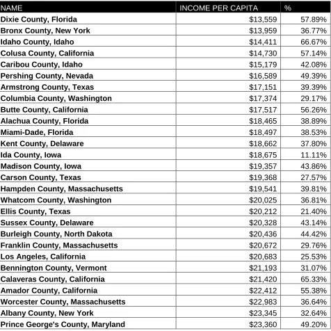
[image:16.612.94.570.239.715.2]3. Analysis
Table #1 “Global Samples”
NAME INCOME PER CAPITA %
Dixie County, Florida $13,559 57.89%
Bronx County, New York $13,959 36.77%
Idaho County, Idaho $14,411 66.67%
Colusa County, California $14,730 57.14%
Caribou County, Idaho $15,179 42.08%
Pershing County, Nevada $16,589 49.39%
Armstrong County, Texas $17,151 39.39%
Columbia County, Washington $17,374 29.17%
Butte County, California $17,517 56.26%
Alachua County, Florida $18,465 38.89%
Miami-Dade, Florida $18,497 38.53%
Kent County, Delaware $18,662 37.80%
Ida County, Iowa $18,675 11.11%
Madison County, Iowa $19,357 43.86%
Carson County, Texas $19,368 27.57%
Hampden County, Massachusetts $19,541 39.81%
Whatcom County, Washington $20,025 36.81%
Ellis County, Texas $20,212 21.40%
Sussex County, Delaware $20,328 43.14%
Burleigh County, North Dakota $20,436 44.42%
Franklin County, Massachusetts $20,672 29.76%
Los Angeles, California $20,683 25.53%
Bennington County, Vermont $21,193 31.07%
Calaveras County, California $21,420 65.33%
Amador County, California $22,412 55.38%
Worcester County, Massachusetts $22,983 36.64%
Albany County, New York $23,345 32.64%
XVII
Storey County, Nevada $23,642 51.30%
Washoe County, Nevada $24,277 52.12%
Alpine County, California $24,431 32.82%
New London County, Connecticut $24,678 56.38%
Essex County, New Jersey $24,943 26.66%
Barnstable County, Massachusetts $25,318 41.04%
Calvert County, Maryland $25,410 64.36%
Tolland County, Connecticut $25,474 44.77%
Hartford County, Connecticut $26,047 37.38%
Burlington County, New Jersey $26,339 21.27%
Alameda County, California $26,680 35.61%
Juneau County, Alaska $26,719 48.18%
Douglas County, Georgia $27,288 35.31%
Talbot County, Maryland $28,164 46.27%
Middlesex County, Connecticut $28,251 46.41%
DC, WASHINGTON $28,659 30.40%
Contra Costa County, California $30,615 37.97%
Norfolk County, Massachusetts $32,484 21.31%
Bergen County, New Jersey $33,638 29.64%
San Francisco County, California $34,556 37.91%
Fairfield County, Connecticut $38,350 25.78%
New York County, New York $42,922 26.59%
In order to perform the analysis we first need to state the hypothesis that will be tested.
As a Null hypothesis or H0 this study will part from the following reasoning. There is a
relation between income per capita and the wireless security level of a particular
geographic entity. Always, no matter the amount of samples, if we separate the samples
in two groups, Group A conformed by items with an income per capita lower than the
median and Group B conformed by items with an income per capita higher than the
median income per capita. Group A will have all its items with a security level below the
XVIII This indicates that in any given number of samples, it will always appear a Group B with
a higher income per capita and wireless security level than the samples median that
represents the 50% of the population. This is why we will consider the probability of
taking a developed country with high security from the total population is 50%.
H0: p = 0.5. Developed counties have a higher security level.
The alternate hypothesis, as the opposite of the null hypothesis, indicates that no
relation exists between income per capita and wireless security level of a particular
geographical entity. In other words the result will be different than the 50/50 relation that
conforms the null hypothesis.
This indicates that H1 will be true, if the probability of having an element of the sample
higher than the median security level is different from 0.5 or P!=0.5;
H1: p <> 0.5, more developed counties have less security.
In terms of proportion this test will be limited to 50, due the limitations of using wiggle as
a source of data. Wiggle receive information from users located in several counties,
many of them do not have information, because no one have uploaded any data.
Now we need to define Type I and Type II errors. A Type I error or error of the first kind
consist on rejecting the null hypothesis when the analyst have enough knowledge and
knows it is true. In other words, it happens when we see in the experiment a result that
shows a difference with the null hypothesis when in truth there is actually none. An
example of this could be test that shows that a person has a particular disease when he
XIX Type II errors or error of the second kind, consist on accepting the null hypothesis when
the result of the test turn to be false. For example, a test to a person with a particular
disease that turned to be false when he is actually having health issues.
By defining Type I and Type II error we cover all the possible result in the experiment. In
[image:19.612.87.609.306.363.2]the following table it is shown how the result are distributed.
Table #2 “Type Errors”
With a Disease With no Disease
EXPERIMENT
Healthty Type I (he actually is sick) OK
Not Healthy OK
Type II (he actually is not sick)
To separate the groups first we have to calculate the median value of the income per
capita and security level, by using the excel function “average” we obtain the following
values. It can be done by hand also, by sorting from lower to higher the income per
capita. In case there is an odd amount of entries taking the value of the entry that
separates the sample in two equal parts is taken as the median value, if a pair amount of
entries exist then the two values that separates the sample in two groups are
summarized and divided by two.
For example, in 1,2,3,4,5 we see there is an odd amount of entries because of that we
shoce as the median 3.
Another example, in 1,2,3,4,5,6 we see there is a pair number of entries, we execute
XX Remember the median value is the one located in the exact middle of the range of
results obtained in a numerical sample.
Table #3 “Median of the Sample”
Income Per capita
Median Security median
$22,698 38.25%
Now with the income per capita we can separate the items in two groups in GROUP A
the counties with an income per capita bellow the median which we will consider
underdeveloped. Group B has the more developed counties. They all have an income
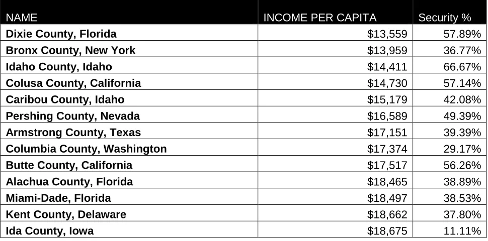
[image:20.612.89.574.479.719.2]per capita higher than the median.
Table #4 “GROUP A”
NAME INCOME PER CAPITA Security %
Dixie County, Florida $13,559 57.89%
Bronx County, New York $13,959 36.77%
Idaho County, Idaho $14,411 66.67%
Colusa County, California $14,730 57.14%
Caribou County, Idaho $15,179 42.08%
Pershing County, Nevada $16,589 49.39%
Armstrong County, Texas $17,151 39.39%
Columbia County, Washington $17,374 29.17%
Butte County, California $17,517 56.26%
Alachua County, Florida $18,465 38.89%
Miami-Dade, Florida $18,497 38.53%
Kent County, Delaware $18,662 37.80%
XXI
Madison County, Iowa $19,357 43.86%
Carson County, Texas $19,368 27.57%
Hampden County, Massachusetts $19,541 39.81%
Whatcom County, Washington $20,025 36.81%
Ellis County, Texas $20,212 21.40%
Sussex County, Delaware $20,328 43.14%
Burleigh County, North Dakota $20,436 44.42%
Franklin County, Massachusetts $20,672 29.76%
Los Angeles, California $20,683 25.53%
Bennington County, Vermont $21,193 31.07%
Calaveras County, California $21,420 65.33%
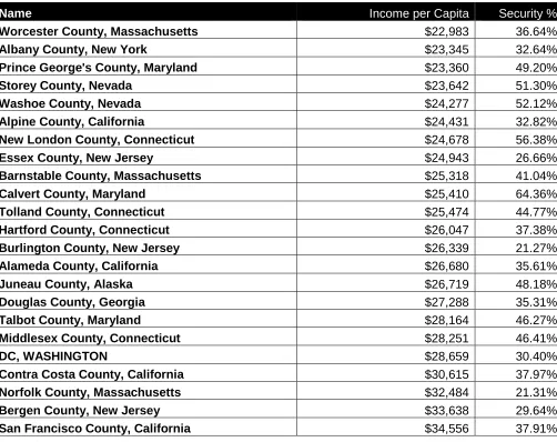
[image:21.612.96.598.320.718.2]Amador County, California $22,412 55.38%
Table #5 “GROUP B”
Name Income per Capita Security %
Worcester County, Massachusetts $22,983 36.64%
Albany County, New York $23,345 32.64%
Prince George's County, Maryland $23,360 49.20%
Storey County, Nevada $23,642 51.30%
Washoe County, Nevada $24,277 52.12%
Alpine County, California $24,431 32.82%
New London County, Connecticut $24,678 56.38%
Essex County, New Jersey $24,943 26.66%
Barnstable County, Massachusetts $25,318 41.04%
Calvert County, Maryland $25,410 64.36%
Tolland County, Connecticut $25,474 44.77%
Hartford County, Connecticut $26,047 37.38%
Burlington County, New Jersey $26,339 21.27%
Alameda County, California $26,680 35.61%
Juneau County, Alaska $26,719 48.18%
Douglas County, Georgia $27,288 35.31%
Talbot County, Maryland $28,164 46.27%
Middlesex County, Connecticut $28,251 46.41%
DC, WASHINGTON $28,659 30.40%
Contra Costa County, California $30,615 37.97%
Norfolk County, Massachusetts $32,484 21.31%
Bergen County, New Jersey $33,638 29.64%
XXII
Fairfield County, Connecticut $38,350 25.78%
XXIII Now the next step consist in verifying how many items of group A have a lower security
percentage than the wireless security median which is 38.25% and how many in group B
have a wireless security percentage above the median. The following table shows the
results.
Table #6 “Group A elements satisfying null hypothesis”
Less than median security % (satisfy null Ho)
Higher than median security % (Do not satisfy Ho)
10 15
We can see that the percentage of items with wireless security level less than the
median is 40% and the remaining is the percentage of items that did not resulted to be
true and the median security level of this group A is 41.01%
Table #7 “Group B elements satisfying null hypothesis”
Higher than median security % Less than security %
15 10
We can see that 60% of the group B items had a wireless security level higher than the
median wireless security value and the remaining 40% were the items that resulted to be
false and the median of this group is 38.72%
Table #8 “Binomial Test Results”
Probability of success on a single
trial 0.5
Number of trials 50
XXIV The value of the variable ”number of success” is 25, meaning that from the entire sample
only 25 elements satisfies the null hypothesis. In Group A we can see 10 elements that
have a wireless security level below the median value. These 10 elements, plus the 15
elements that satisfy the null hypothesis in Group B, form a total of 25 elements that
satisfy the null hypothesis.
Because of the nature of the test, the Probability of success on a single trial is 0.5. We
have only two possible results in our test and the elements can only satisfy or not the
null hypothesis, in other words the result can be true or false.
The Binomial value represents the probability of having X elements between the
samples that support the null hypothesis. In this case is p = 0.1122 or 11.22% which
means that there is practically no chance of getting a sample with more than a 50% of
success. By knowing this we can determinate that no relation between income per capita
and wireless security level exist.
The probability of selecting a geographical entity that satisfy the null hypothesis is a
50%, in order to consider true the null hypothesis a higher value of P would be require
and a success rate of at least 85% of the sample.
By making another binomial test with the following data:
Success rate = 45
Trials = 50
XXV We will see that the chance of having more successful items in the samples becomes
even smaller, the P value in this case turns to be 9*10^-9 which is practically impossible
to obtain. Another factor that rejects the null hypothesis is that the median of the less
developed counties is higher than the median of the more developed counties.
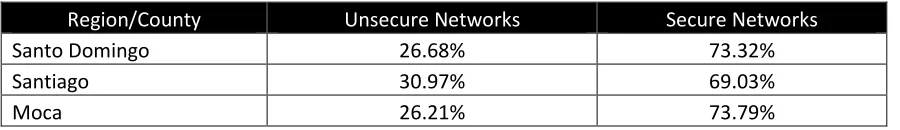
[image:25.612.84.534.237.302.2]Now we will proceed to analyze the Dominican Republic data:
Table #9 “Dominican Republic war drive information”
Region/County Unsecure Networks Secure Networks
Santo Domingo 26.68% 73.32%
Santiago 30.97% 69.03%
Moca 26.21% 73.79%
Since in the Dominican Republic the income per capital is calculated by the sector that
generates the income and not the geographical entity we will use the Dominican
Republic income per capita and the wireless security average from the samples as the
representation of the country. The income per capita of Dominican Republic is 4815.6$
XXVI
V – RESULTS
The first analysis we will performed is by comparing the two median values of Group A
and Group B. By performing the analysis described in the methodology we obtained the
following results.
Table #10 “Mean Values”
Total Sample Group A Group B
Median 38.25% 41.01% 38.72%
If we part from the idea that the null hypothesis is true and there is a relation between
income per capita and wireless security level we can state the following. The median
value of Group A should have a similar distance or difference from the total sample
median and the value of the first item of Group A. Also we can state that there should be
a similar distance or difference between the median of Group B and the medians values
of the total sample and the last item value of Group B.
This can be explained with the following example:
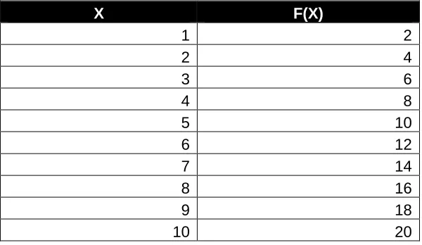
If we performed 10 test to this equation f(x) = x*2 with number from 1 to 10 we will get
XXVII
Table #11 “F(x) Results”
X F(X)
1 2
2 4
3 6
4 8
5 10
6 12
7 14
8 16
9 18
10 20
We can appreciate that the median value of F(X) is 11 because of Median = (12+10)/2,
also we can see that the median values of the items below the total median is 6 and the
median of the items above is 16. We can see that the distance of the first group median
from the total median and the lower value of F(x) is of 4, the same happens to the
median of the group above the total median and the higher value of F(x) in the sample.
This occurs because a linear relation exists between them.
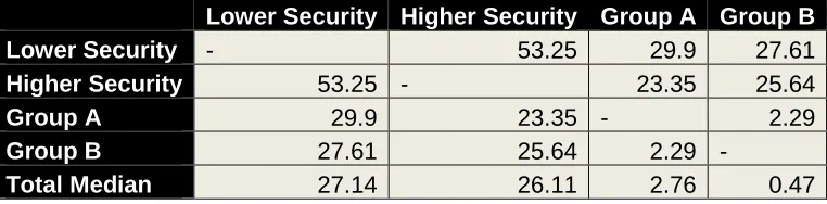
In our experiment we don’t see this type of behavior, as we can see in table #11, the
distance between the total Median and Group B median is of 0.47 and the difference
between Group B median and the item with higher security level in Group B is of 25.64.
On the other hand group A had a similar behavior the distance from the total median to
Group A median is of 2.76 and the difference between the lower security item and Group
A median is of 29.9. From this test we can be sure that their does not exist a relation
between income per capita and wireless security, another interesting behavior we see is
that the median of Group A which are the undeveloped counties is greater than the
median of Group B or developed counties. If any type of relation that sustained the null
XXVIII
Table #12 “Distance between Median”
Lower Security Higher Security Group A Group B
Lower Security - 53.25 29.9 27.61
Higher Security 53.25 - 23.35 25.64
Group A 29.9 23.35 - 2.29
Group B 27.61 25.64 2.29 -
Total Median 27.14 26.11 2.76 0.47
Since by analyzing the median from the samples we did not obtained any evidence of
the null hypothesis been true, we will proceed to analyze the result from the binomial test
which is the probability of obtaining the result we had from a given number of samples.
We see that the probability of obtaining this result was of 11.22%. This probability gets
even lower if is calculated with a success rate of 90%, we had a probability of less than
1% this practically a direct rejection to the null hypothesis because of the lack of chance
of getting this result.
Now by taking the Dominican Republic Data, we can see that the country is part of
Group A because of the overall the counties in this group have a income per capita
higher than the 4815.6$ USD of the Dominican Republic, in fact the hole sample of the
united states has a higher income per capita. This means that the overall security of the
United States must be higher than the Dominican Republic.
By calculating the average security level and income per capita of the sample we can
determinate the following
• USA income per capita = 23,180USD
XXIX By getting these values we see that Dominican Republic has a much lower income per
capita than the USA, but has a higher wireless security level, in fact all the samples
taken in Dominican Republic had a higher wireless security level than any of the
samples taken in the USA. This might happened because of the nature of the USA war
drive data, this data could be representing a particular zone since several users upload
data of the same area, and on the other hand, the data gathered of the Dominican
Republic was done by a single user in different areas, the samples are not repeated.
This result reveals the lack of relation of only income per capita and wireless security,
since the income per capita of a county its only one of the factors that can alters a group
of individual’s behavior. We can say that more variables need to be involved in this
investigation.
Variables like the education level, rhythm of life and age of the population could be
included, a younger population can be more curious about new technologies and have
more information about the risks of having unsecure wireless networks. On the other
hand a population with an agitated rhythm of life could be more careless than a
population with a more calm rhythm.
Others studies can be done involving how comfortable are access points interfaces, in
order to measure how many consider they interfaces comfortable, user friends but at the
XXX
VI - REFERENCE
[1] - "The Wireless security survey of London." October 2008. RSA, Security Division of
EMC. 8 Jun 2009
<http://www.rsa.com/solutions/wireless/survey/WLANLN_WP_1008.pdf>.
[2] – "The Wireless security survey of New York." October 2008. RSA, Security Division
of EMC. 8 Jun 2009
<http://www.rsa.com/solutions/wireless/survey/WLANNY_WP_1008.pdf>.
[3] – "The Wireless security survey of Paris." October 2008. RSA, Security Division of
EMC. 8 Jun 2009
<http://www.rsa.com/solutions/wireless/survey/WLANPA_WP_1008.pdf>.
[4] - Koerner, Brendan. "License to Wardrive." Legal Affairs. June 2005. 8 Jun 2009
<http://www.legalaffairs.org/issues/May-June-2005/review_koerner_mayjun05.msp>.
[5] – "Backtrack." Backtrack. 8 Jun 2009 <http://www.remote-exploit.org/backtrack.html>.
[6] – Susan, Lincke. "Network security auditing as a community-based learning project."
2007.
University of Wisconsin-Parkside, Kenosha, Wisconsin . 8 Jun 2009
<http://portal.acm.org/citation.cfm?doid=1227310.1227472>.
[7] – "Facing the challenge of wireless security." Jul 2001. Miller, S.K. 13 March 2010
<http://ieeexplore.ieee.org.ezproxy.rit.edu/stamp/stamp.jsp?tp=&arnumber=933495>.
[8] – "Income per Caipta." 28 March 2010
<http://www.investorglossary.com/per-capita-income.htm>.
[9] – “Dominican Republic Income Per Capita” 28 April 2010
XXXI
VII – APENDIX
A. Income per capita Dominican Republic By Year
(http://www.bancentral.gov.do/estadisticas_economicas/sector_real/pib.xls)
Producto Interno Bruto Percápita 1991-2009
Población PIB Corriente PIB Corriente PIB Referencia 1991 PIB Referencia 1991 PIB Corriente PIB Corriente (Miles) (Millones de RD$) (Percápita RD$) (Millones RD$) (Percápita RD$) (Millones de
US$) (Percápita US$)
1991 6,968 123,426.0 17,713.6 123,426.0 17,713.6 9,575.6 1,374.3 1992 7,129 144,063.3 20,208.7 136,402.0 19,134.0 11,392.7 1,598.1 1993 7,293 162,205.1 22,240.0 146,253.8 20,052.9 12,882.5 1,766.3 1994 7,425 182,840.3 24,626.4 149,622.4 20,152.4 14,213.5 1,914.4 1995 7,558 211,024.6 27,920.3 157,842.1 20,883.8 15,857.3 2,098.1 1996 7,694 233,833.3 30,391.5 169,098.4 21,977.9 17,411.5 2,263.0 1997 7,832 274,423.9 35,037.0 182,633.5 23,317.7 19,401.4 2,477.1 1998 7,973 311,282.8 39,040.8 195,437.2 24,511.5 20,724.0 2,599.2 1999 8,117 343,745.3 42,350.5 208,561.5 25,695.4 21,575.8 2,658.2 2000 8,263 388,301.9 46,994.8 220,359.0 26,669.3 23,799.3 2,880.3 2001 8,411 415,520.9 49,400.3 224,345.8 26,672.0 24,561.0 2,920.0 2002 8,563 463,624.3 54,145.6 237,331.4 27,717.4 24,985.6 2,918.0 2003 8,717 617,988.9 70,898.7 236,730.1 27,158.8 20,432.1 2,344.1 2004* 8,873 909,036.8 102,447.1 239,835.9 27,029.2 22,608.7 2,548.0 2005* 9,033 1,020,002.0 112,922.3 262,051.3 29,011.2 33,774.7 3,739.1 2006* 9,195 1,189,801.9 129,393.9 290,015.2 31,539.9 35,897.2 3,903.9 2007* 9,361 1,364,210.3 145,740.7 314,592.8 33,608.4 41,228.1 4,404.5 2008* 9,529 1,576,162.8 165,409.8 331,126.8 34,750.0 45,717.6 4,797.8 2009* 9,700 1,678,762.6 173,068.0 342,564.1 35,315.8 46,711.6 4,815.6 *Cifras preliminares
XXXII
B. Growth Rates Dominican Republic by Year
(http://www.bancentral.gov.do/estadisticas_economicas/sector_real/pib.xls)
Tasas de Crecimiento (%)
Población PIB Corriente PIB Corriente PIB Referencia 1991 PIB Referencia 1991 PIB Corriente PIB Corriente
(Miles) (Millones de RD$)
(Percápita
RD$) (Millones RD$) (Percápita RD$)
(Millones de US$)
(Percápita US$)
1992 2.3 16.7 14.1 10.5 8.0 19.0 16.3
1993 2.3 12.6 10.1 7.2 4.8 13.1 10.5
1994 1.8 12.7 10.7 2.3 0.5 10.3 8.4
1995 1.8 15.4 13.4 5.5 3.6 11.6 9.6
1996 1.8 10.8 8.9 7.1 5.2 9.8 7.9
1997 1.8 17.4 15.3 8.0 6.1 11.4 9.5
1998 1.8 13.4 11.4 7.0 5.1 6.8 4.9
1999 1.8 10.4 8.5 6.7 4.8 4.1 2.3
2000 1.8 13.0 11.0 5.7 3.8 10.3 8.4
2001 1.8 7.0 5.1 1.8 0.0 3.2 1.4
2002 1.8 11.6 9.6 5.8 3.9 1.7 (0.1) 2003 1.8 33.3 30.9 (0.3) (2.0) (18.2) (19.7) 2004* 1.8 47.1 44.5 1.3 (0.5) 10.7 8.7 2005* 1.8 12.2 10.2 9.3 7.3 49.4 46.7 2006* 1.8 16.6 14.6 10.7 8.7 6.3 4.4 2007* 1.8 14.7 12.6 8.5 6.6 14.9 12.8 2008* 1.8 15.5 13.5 5.3 3.4 10.9 8.9 2009* 1.8 6.5 4.6 3.5 1.6 2.2 0.4 *Cifras preliminares
XXXIII
C. Binomial Test
Conditions of Use: Use the binomial test when you have dichotomous data - that is,
when each individual in the sample is classified in one of two categories (e.g. category A
and category B) and you want to know if the proportion of individuals falling in each
category differs from chance or from some pre-specified probabilities of falling into those
categories.
Assumptions: The normal approximation for the Binomial test assumes that the
proportion of the time that individuals are expected to fall into category A (symbolized by
"p") multiplied by the total number of individuals in category A and B combined
(symbolized by "n") is greater than 10 (i.e. pn>10) and that the proportion of the time that
individuals are expected to fall into category B (symbolized by "q") multiplied by the total
number of individuals is greater than 10 (i.e. qn>10). If either of these conditions are not
met then the normal approximation for the binomial test should not be used (use the
Binomial distribution instead).
Example: In a recent study examining colour preferences in infants, 30 babies were
offered a choice between a red rattle and a green rattle. Twenty-five of the 30 selected
the red rattle. Do these data provide evidence for a significant colour preference? Test
at the 0.01 level of significance.
Step 1. State the hypotheses, and specify alpha. The null hypothesis states that the
proportion of babies preferring red rattles is not different from what is expected for a
population where there is no preference for rattle colour. In symbols,
(
)
0
.
5
and
(
)
0
.
5
:
0
p
=
p
red
=
q
=
p
green
=
XXXIV The alternative hypothesis is that the proportions for the colour preferences are different
from what is expected for these chance population proportions.
We will set .
Step 2. Locate the critical region. Because pn and qn are both greater than 10, we can
use the normal approximation to the binomial distribution. With , the critical
region is defined as any z-score value greater than +2.3263 or less than -2.3263.
Step 3. Calculate the test statistic. In the sample 25 out of 30 babies prefer the red
rattle, so the sample proportion is.
)
5
.
0
(and
5
.
0
:
1
p
≠
q
≠
H
01
.
0
=
α
01
.