Element mobility and spatial zonation associated with the Archean Hamlet orogenic Au deposit, Western Australia: Implications for fluid pathways in shear zones

Contents lists available atScienceDirect

Chemical Geology

journal homepage:www.elsevier.com/locate/chemgeo

Element mobility and spatial zonation associated with the Archean Hamlet

orogenic Au deposit, Western Australia: Implications for fluid pathways in

shear zones

Shawn B. Hood

_{, Matthew J. Cracknell}

_{, Michael F. Gazley}

_{, Anya M. Reading}

b_{ARC Industrial Transformation Research Hub for Transforming the Mining Value Chain (TMVC) at CODES, Hobart, Tasmania, Australia} c_{School of Natural Sciences (Math and Physics), University of Tasmania, Hobart, Tasmania, Australia}

d_{RSC Mining and Mineral Exploration, 93 The Terrace, Wellington, New Zealand} e_{Victoria University of Wellington, PO Box 600, Wellington, New Zealand}

A R T I C L E I N F O

Editor: Karen Johannesson Keywords:

Mass balance Metasomatism Ore deposit Orogenic gold Shear zone Fluid flow Archean St Ives Hamlet Au lode

A B S T R A C T

Mass balance equations can be used to understand metasomatism. Here we use 2726 multi-element chemical analyses to quantify the effect of metasomatism associated with Au mineralisation at the Hamlet Gold Mine (Hamlet), Yilgarn Craton, Western Australia. Principal components analysis is first used to identify covarying elements and six groups of elements are identified: (1) relatively immobile elements, with Zr and Hf providing an appropriate reference frame for mass balance calculations; (2) elements associated with mafic rocks, such as Ca, Co, Fe, Ge, Mg, Mn, and Zn; (3) elements related to potassic alteration, Ba, Cs, K, Rb, and Tl; (4) elements related to sodic alteration, Be, Na, and Sr; (5) chalcophile elements, including Bi, weakly associated with Au; and (6) Au, Te, and S representing the main Au-mineralising event. A statistically-rigorous approach is then used to quantify element addition and depletion and provides 95% confidence limits for changes in mass. To achieve this, the basaltic host rocks are divided into four subunits based on Cr content. Sample subsets are then created to select altered rocks and least-altered protolith rocks, using discrimination diagrams. Pairings of least altered-altered samples from each basalt subunit are used to construct matrices via bootstrapping. Mass balance results from these matrices indicate similar element mobility associated with Au mineralisation across the four basalt sub-units, with up to 24% mass loss. Key potassic and sodic group elements are enriched in the Au mineralised zones at the expense of elements with a mafic-association. Spatial patterns of mass change are linear and repetitive within the steeply-dipping Hamlet Shear Zone, interpreted to represent a mesh-like geometry of metasomatism within the plane of the shear zone. Localised enrichment of K, Na, and Bi are related to Au distribution while Ca depletion zones reflect the movement of reactive fluid along the shear plane.

1. Introduction

Orogenic Au deposits can provide a sample-rich opportunity to in-vestigate geochemical changes associated with deformation-focussed metasomatic activity. While univariate geochemical data or element ratios can be an effective first-pass method to investigate chemical distribution and relative abundance for a region (Reimann, 2005), these approaches do not quantify element addition or depletion. Methods to quantify geochemical changes include: (1) calculating ‘enrichment factors’ using ratios, where the element concentration of interest is divided by the concentration of an immobile element (Chandrajith et al., 2001;Brauhart et al., 2017;Carranza, 2017); (2) Pearce Element

Ratios (Stanley and Madeisky, 1996;Whitbread and McQueen, 2002; Urqueta et al., 2009); and (3) calculating mass balance, where the ratio of immobile element concentration for an altered and unaltered (or least-altered) sample provide a reference frame for computing element addition or loss (Gresens, 1967;Grant, 1986, 2005; McKinley et al., 2016).

Geochemical mass change in open-systems has been discussed ex-tensively in the literature (Gresens, 1967; Grant, 1986;Brimhall and Dietrich, 1987;Brimhall et al., 1988;Ague and van Haren, 1996). An application of mass balance calculations is to quantify element changes in metasomatically-altered rock, relative to the unaltered (or least-al-tered) rock representing the protolith. The results provide information

https://doi.org/10.1016/j.chemgeo.2019.03.022

Received 4 December 2018; Received in revised form 14 March 2019; Accepted 20 March 2019

⁎_{Corresponding author at: Centre for Ore Deposit and Earth Sciences (CODES), University of Tasmania, Hobart, Tasmania, Australia.} E-mail address:[email protected](S.B. Hood).

Chemical Geology 514 (2019) 10–26

Available online 27 March 2019

0009-2541/ © 2019 The Authors. Published by Elsevier B.V. This is an open access article under the CC BY-NC-ND license (http://creativecommons.org/licenses/BY-NC-ND/4.0/).

about the effects of overprinting metasomatism experienced by the al-tered rock or suite of alal-tered rocks. In this study, a statistically-robust elemental mass balance investigation is presented for the Hamlet Gold Mine (Hamlet;Fig. 1). The methodology provides a technique to model

hydrothermal fluid flow pathways in three dimensions (3-D), and re-sults improve our understanding of element mobility in shear-asso-ciated greenstone Au (orogenic Au) deposits. To support mass balance results, Principal Components Analysis (PCA;Pearson, 1901;Jolliffe,

76/081

44/095

42/063

70/092 50/095

23/274

50 /1₂₇ 39/307

78/145 77/207

75/203

384000 385000 386000 387000

6

5

2

5

0

0

0

6

5

2

6

0

0

0

Athena Shear

Ham l et Sh ear

Yorick Shear Argo Shear Complex

Apollo Shear

Open pit

Open pit with underground portal Underground via link drive

42/248

54/264

Dip/dip direction of Paringa Basalt contact Dip/dip direction of mineralised shear zone Intermediate

Intrusions

Du rk

in _Ant

iclin e Axial

T_race

N

Lower PBS Athena Basalt Upper (and Middle) PBS Condensor Dolerite Black Flags Group

Lower PBS or Defiance Dolerite

Fig. 1.Bedrock map of St Ives, Western Australia, showing the Paringa Basalt (PBS) and mineralised shear zones (red) within the greater Argo-Athena-Hamlet shear complex. The axial trace of the Durkin Anticline is shown as a dashed line. Map drafted using unpublished company mapping and the drill data used in this study. (For interpretation of the references to colour in this figure legend, the reader is referred to the web version of this article.)

Black Flags Group

Condensor Dolerite

Athena Basalt

Paringa Basalt

Defiance Dolerite

Argillite, wacke, felsic and intermediate intrusive rocks, volcanic conglomerate, breccia and tuff. 1500 m thick

Intrusive tholeiitic differentiated dolerite and gabbro. 5 - 500 m thick

Pillow or aphyric basalt. Up to 300 m thick

Siliceous high Mg basalt, minor interflow sediments. 500 - 1000 m thick

Differentiated dolerite. 60 - 100 m thick.

Hamlet Shear Zone Athena Shear Zone

Argo Shear Complex Apollo Shear

Biotite Envelope

Foliation Envelope N

Ore shoot trend-plunge

~5m Sub-horizontal

veins

Sub-vertical veins Breccia

2011) is used to produce groups of elements associated with protolith rock composition or overprinting alteration effects.

2. Geochemical mass balance

The conventional graphical mass balance approach ofGrant (1986, 2005)is not well-suited to highly-variable rock composition, noisy data and/or large datasets. First, the immobile element reference frame se-lected can strongly affect the outcome of mass change estimates. This is because major and trace element concentrations differ by orders of magnitude. Very-low concentrations near the analytical detection limit contribute less to the position of the isocon than higher values, analy-tical errors, and the variable mobility of “immobile elements” (e.g., Baumgartner and Olsen, 1995; Mukherjee and Gupta, 2008; Ahmed et al., 2019). Second, parent protolith rocks are chemically hetero-geneous and altered rocks are not uniformly altered in terms of extent or type.

Compositional analyses also include analytical error (Ague and van

Haren, 1996). Samples picked to represent protolith may yield sig-nificantly different results, due to variable composition. Simplified approaches using arithmetic averaging of geochemical data do not address this issue. Univariate geochemical datasets do not generally follow a Gaussian distribution model and standard statistical ap-proaches are invalid for multivariate compositional data (Vistelius, 1960;Aitchison, 1986;Aitchison, 1989;Reimann and Filzmoser, 2000). The sample vs. sample approach ofGrant (1986, 2005)also becomes laborious when handling many samples, as are commonly available at an advanced mineral exploration project or mining operation. Many computer programs have been developed to improve the speed of processing mass balance equations (Potdevin, 1993; Lopez-Moro, 2012), or to facilitate the selection of an immobile reference frame (Janousek et al., 2006;Carrasco and Girty, 2015). While useful, these approaches do not statistically represent compositional variability of sample populations and the uncertainty of mass balance results is not provided.

Recent work byAhmed et al. (2019) addresses this issue by ex-amining boxplots of sample data to assess the uncertainty of individual mass balance estimates and uses spreadsheets to speed up calculations. However the approach ofAhmed et al. (2019)does not provide a robust estimate of element change for the entire alteration domain. To address this issue, we apply the modified mass balance approach ofAgue and van Haren (1996); this approach was selected because it features au-tomation for dealing with large sets of samples, is statistically-robust, and provides a measure of confidence for results. An innovative use of these results is to relate them to the covariance of elements (as mea-sured using PCA) and to furthermore derive 3-D representation of ele-ment enrichele-ment and depletion. Results can then inform between geochemical data and the structural-mineralogical controls on miner-alisation in orogenic Au deposits.

3. Case study area

The St Ives Au-Ni Camp is located near the township of Kambalda, Western Australia, 57 km south of Kalgoorlie. The St Ives area has produced over 12 Moz of Au to date, from multiple open pit and un-derground mines (Carolus, 2018). Discovered in 2009, the Hamlet un-derground mine occurs within the multi-million-ounce Argo-Athena-Hamlet shear complex (Fig. 1) in the southern portion of St Ives and is currently in production.

St Ives is in the Kambalda Domain of the Kalgoorlie Terrane, Yilgarn Craton, Western Australia (Czarnota et al., 2010). The greenstone stratigraphy of the Kambalda Domain comprises regionally metamor-phosed mafic-ultramafic, felsic intrusive and clastic sedimentary units (Squire et al., 1998;Krapež and Hand, 2008;Czarnota et al., 2010). The Paringa Basalt, which hosts Hamlet (Fig. 2), is part of a regional high-Th siliceous basalt group (Barnes et al., 2012) with a type area located between Kalgoorlie and Kambalda. The Paringa Basalt comprises sub-marine pillowed and massive facies, some of which are thick and in-ternally differentiated (Lesher, 1983). The major element compositions of the unit range from magnesian andesite to basalt with anomalously high Si content and include a component of fractionates and cumulates (Barnes et al., 2012). Regional greenschist facies metamorphism, overprinting the Paringa Basalt, is recorded by an assemblage of am-phibole-chlorite-albite-plagioclase (Prendergast, 2007).

The Hamlet deposit is hosted entirely within the Paringa Basalt. This formation contains variolitic intervals and pillowed basalt flows up to tens of metres thick, and thicker differentiated dolerite units up to hundreds of metres. The formation grades from high-Mg basalt at the base, to more-evolved tholeiitic basalts at the top; these two geo-chemical domains are informally separated as Upper- and Lower-Paringa Basalt (Barnes et al., 2012;Walshe et al., 2014). As it is not always possible to separate these subunits visually during diamond drill core logging, logs contain codes for Upper- or Lower Paringa, or simply Paringa. Typically, they are discriminated into three informal subunits

4.5 cm

A.

4.5 cm

2.5 cm

1 m

B.

C.

D.

ab1

± py± po

ab2-qz

bt

chl dominant

bt dominant

ab1

bt dominant

using whole rock geochemical data. These subunits are defined using Th-Cr-Ti ternary plots as the Upper, Middle, and Lower Paringa Basalt (Walshe et al., 2014).

Structurally, the Kambalda Domain is bound to the east by the Boulder-Lefroy Fault Zone and to the west by the Zuleika Shear Zone (Swager et al., 1995;Myers, 1997). Multiphase deformation associated with movement along these shear zones is manifested by five main deformation events (Blewett et al., 2010; Miller et al., 2010; McGoldrick et al., 2013b). Gold mineralisation is interpreted to have occurred during peak metamorphism, late in the deformation history, within second-order structures such as vein arrays, sinistral-reverse shear zones and thrust faults related to the episodic rupture of segments on the main faults (Nguyen et al., 1998; Cox and Ruming, 2004; Connors et al., 2005;Ruming, 2006;Miller et al., 2010).

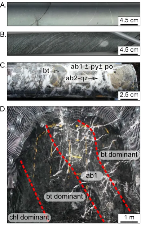
The Hamlet Shear Zone cuts the Paringa Basalt as a steeply dipping, 5 m to 25 m wide zone of shear foliation (Fig. 2). The shear zone may be continuous, or a series of discrete narrow shears separated by un-deformed basalt. Potassic alteration, in the form of biotite replacement of chlorite or pyroxene, is present as an envelope around veining in the shear zone (Fig. 3) ≤15 m thick. Gold mineralisation at Hamlet com-prises quartz and carbonate vein arrays with associated biotite‑carbo-nate-albite-sulfide wall-rock alteration in the shear zone. Pervasive, pale yellow-brown albite is most strongly developed around stockwork quartz-albite veining and quartz-albite matrix breccias (Fig. 3). When plotted in 3-D the samples with the highest Au grades occur along multiple trends within the Hamlet Shear Zone, with no single dominant orientation.

4. Methods

4.1. Initial data and pre-processing

The unfiltered database used in this study contains 6051 samples

and 61 elements from whole-rock analyses. Multi-element assays were produced using a four-acid digest (Activation Laboratories' ME-MS61 procedure in Perth, Western Australia; Appendix A. Dataset QAQC). Whole-rock multi-element geochemistry is from both Inductively Coupled Plasma (ICP) Mass Spectrometry (-MS) and Atomic Emission Spectroscopy (-AES) analyses. The ICP dataset contains 60 elements Ag, Al, As, Ba, Be, Bi, Ca, Cd, Ce, Co, Cr, Cs, Cu, Dy, Er, Eu, Fe, Ga, Gd, Ge, Hf, Ho, In, K, La, Li, Lu, Mg, Mn, Mo, Na, Nb, Nd, Ni, P, Pb, Pr, Rb, Re, S, Sb, Sc, Se, Sm, Sn, Sr, Ta, Tb, Te, Th, Ti, Tl, Tm, U, V, W, Y, Yb, Zn, Zr. Gold was analysed by fire assay (Appendix A. Dataset QAQC). Values less than analytical limit of detection (LOD; censored values) were substituted with values half of detection limit (Grunsky and Smee, 1999;Carranza, 2011) and are listed in Appendix A. When < 30% of element values are censored, replacement of censored values with va-lues half of detection limit has been shown to have minimal effect on the mapping and interpretation of multi-element anomalies related to mineralisation (Carranza, 2011).

Principal components analysis (Pearson, 1901;Jolliffe, 2011) was used to produce geochemical groups in ioGAS™. Conventional algebraic operations and statistical calculations applied to compositional data lead to incorrect results (Pawlowsky-Glahn et al., 2015). This is because chemical compositional data are closed, sum to a constant value, and only contain relative information. Therefore correlation coefficients calculated on raw compositional data are not valid (Aitchison, 1986; Pawlowsky-Glahn et al., 2015). To address this, element concentrations were transformed before PCA using the centred log-ratio (CLR) trans-form (Aitchison, 1986;Aitchison, 2008). A subset of samples did not include the elements Dy, Er, Eu, Gd, Ho, Lu, Nd, Pr, Se, Sm, Tb, Tm, or Yb as part of analytical batches. These elements were omitted from transformation. The final list of CLR transformed elements (n= 48) were: Ag, Al, As, Au, Ba, Be, Bi, Ca, Cd, Ce, Co, Cr, Cs, Cu, Fe, Ga, Ge, Hf, In, K, La, Li, Mg, Mn, Mo, Na, Nb, Ni, P, Pb, Rb, Re, S, Sb, Sc, Sn, Sr, Ta, Te, Th, Ti, Tl, U, V, W, Y, Zn, and Zr.

652

600

0

65250

0

0

-2 0 2 4

1 2

Northin

g (m)

No

rthin

g (m)

Zr (CLR) Cr (CLR)

652600

0

6525

00

0

385000 387000

Easting (m)

385000 387000

Easting (m) A.

C.

B.

D. -2.53

0.86 2.09 2.59 3.18 4.06 6.14

5 15 25 25 15 5

Cr (CL

R

)

0.61 1.22 1.44 1.65 1.87 2.15 3.64

5 15 25 25 15 5

Zr (CL

R)

N

N

Mass balance estimates require characterisation of least-altered protolith samples for comparison with corresponding altered samples. We produced the required lithological groups using geochemical dis-crimination plots in ioGAS™. Mass balance calculations were performed using the Python programming language with the numpy and pandas library modules. Compositional data were used for mass balance cal-culations (not CLR transformed data) because the mass balance equa-tions use element ratios, an appropriate method to deal with closure issues (Grant, 1986;Ague and van Haren, 1996;Grant, 2005). Finally, assessment of mass balance data in 3-D was performed using Data-mine™ and Leapfrog™ software.

4.2. Identification of least-altered, weathered, and variably altered samples

Visual core logging data was present for most, but not all, samples. This information included stratigraphic unit (42 classes), regolith type (12 classes), and rock type (48 classes). A variety of fields denoting logged mineralogy were also available. A representative subset of Hamlet basalt samples was extracted using common logging codes. First, least weathered rocks were identified using the regolith column (3170 samples not designated as part of the regolith profile). Next, logged stratigraphic entity was used to isolate samples logged as Paringa Basalt (3489 samples marked as Upper-, Lower-, or un-differ-entiated Paringa Basalt), and logged rock type was used to select only samples marked as mafic (3473 samples). Twenty-seven samples with Ni < 50 ppm plot west of the Hamlet study area indicating these were mis-logged as Paringa Basalt, and they were rejected. A total of 3024

records were present after filtering by rock type. However, after omit-ting samples with missing analyses (i.e., where elements of interest had not been assayed for (see Appendix A. Dataset QAQC)), the final number of transformed samples was 2726.

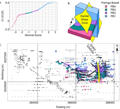
The Paringa Basalt is geochemically heterogeneous and so was di-vided into smaller geochemical domains related to igneous fractiona-tion. The variation in Cr composition of the Paringa Basalt is grada-tional from north to south (Fig. 4). A probability plot of Cr CLR produces approximately similar sized subunit volumes using normal score thresholds of −1.0, 0.0, and 1.0 (Fig. 5). These thresholds divide the Paringa Basalt from stratigraphic base to top into PB1 (n= 433 samples), PB2 (n= 930 samples), PB3 (n= 931 samples), and PB4 (n= 432 samples).

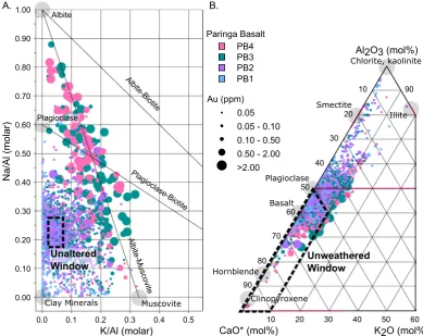
Once samples had been grouped into subunits, least-altered and Au-associated samples needed to be separated (Fig. 6). First, Au and Te LOD values (Au = 0.0005 ppm and Te = 0.025 ppm) were used to identify unmineralised samples. Next, samples along the albite trend of a Na (mol)/Al (mol) vs. K (mol)/Al (mol) plot (Davies and Whitehead, 2006, 2010) were selected to isolate samples likely to contain K or Na-bearing alteration minerals, i.e., albite or biotite. The alkali index (molar ratios of Na/Al and K/Al;Fig. 6A) is an effective tool for iden-tifying major alteration types in Archaean orogenic systems (Davies and Whitehead, 2006; Prendergast, 2007; Davies and Whitehead, 2010). Sodic and potassic alteration assemblages are common in orogenic Au deposits and are coincident with Au mineralisation at Hamlet. Weath-ering of mafic igneous rocks can be discriminated on a ternary plot of Al2O3-CaO-K2O [mol%] (Nesbitt and Young, 1984) (Fig. 6B).

Northin

g

(m)

384000

386000

388000

65270

0

0

6

52500

0

Easting (m)

Normal Score

Cr (CL

R

)

0

0

-2.5

5.5

-1

1

-2

-3

2

3

PB4

PB2

PB1

PB3

Paringa Basalt

N

Hamlet

_Shear

Zone

N

A.

_B.

C.

Anticl

Durkin

in

e

Linear combinations of elements reflecting mineralogy can be more effectively identified using PCA than by through user-defined groups (Grunsky et al., 2014). This approach can use geochemical data to in-form rock composition (Grunsky and Smee, 1999;Grunsky et al., 2014), degree of weathering in regolith (Ohta and Arai, 2007;de Caritat and Grunsky, 2013), and alteration (Loughlin, 1991; Fisher et al., 2014; Caciagli, 2015;Gazley et al., 2015). A benefit of PCA is that the di-mensions of data are reduced, and elements that are covariant can be identified. Multivariate geochemical data represented in Principal Component (PC) space are transformed so that the axis of greatest variance becomes the first PC, the axis of second-greatest variance be-comes PC2, and so on. A triaxial plot of PC1-PC2-PC3 will thus sum-marise the greatest amount of variance in the dataset and be a more comprehensive summary of that dataset than a plot of any three ori-ginal variables.

4.3. Statistically-based mass balance estimates

Our approach to calculating mass balance follows the method of Ague and van Haren (1996). The results obtained using this method produce mathematically-appropriate average estimates of element mass change for an alteration domain, bounded by confidence limits. Aver-aged compositions for representative samples can also be extracted and used to solve mass balance equations for original samples. Results can then be plotted spatially to interpret patterns of conventional mass balance in 3-D.

Gresens' (1967)equation, rearranged byGrant (1986), is shown in Eq. (1), and the variables making up the equation are defined in Table 1.

K/Al (molar)

Na

/A

l (

m

o

lar

)

10

10

20

20

30 30

40 40

50 50

60 60

70

80

90

90

Al2O3 (mol%)

CaO* (mol%)

_{K2O (mol%)}

Unweathered

Window

Clay Minerals Muscovite

Albite-Bi otit

e

Plagi

oclase-Biotite

Alb

ite-Muscovi

te

Smectite

Chlorite, kaolinite

Basalt Plagioclase

Illite

Albite

Hornblende

Unaltered

Window

A.

B.

Clinopyroxene

0.05 0.05 - 0.10 0.10 - 0.50 0.50 - 2.00 >2.00 Au (ppm)

PB4

PB2 PB1 PB3 Paringa Basalt

Fig. 6.Manual assessment of alteration and weathering. Unaltered samples have been chosen as having Au = 0.05 ppm and Te = 0.025 ppm (i.e., both LOD), plotting within the unaltered and unweathered windows. A. Na/Al (molar) vs K/Al (molar) diagram (modified formDavies and Whitehead, 2006) to assess alteration. Samples plotting outside a bounding box of 0.020–0.060 K/Al and 0.175–0.275 Na/Al are considered altered. B. Al2O3-CaO-K2O weathering trend ternary diagram

(afterNesbitt and Young, 1984). The window of unweathered samples ranges from 0–50% Al2O3and 0–10% K2O in the ternary space.

Table 1

Description of variables comprising Eq.(1). Modified fromGrant (1986).

Variable Description

CA _{Concentration of an element in altered rock} CO _{Concentration of an element in least-altered rock} MA _{Mass of altered rock}

MO _{Mass of least-altered rock}

CiA _{Initial concentration of element in altered rock} CiO _{Initial concentration of element in least-altered rock}

CA_/CO _{A proportion representing the change in concentration (addition or} depletion) of an element

MA_/MO _{Isocon reference proportion; the geochemical baseline determined by} user-selected immobile elements

CiA_/CiO _{Initial concentration of an element in the altered sample as a} proportion of an unaltered sample

Eig

en

valu

e

Principal Component 10

1

0 10 20 30 40 50

C C

M M

Ci

Ci 1

A O

A O

A O =

(1) Quantification of mass changes in an open-system requires identi-fication of one or more immobile elements (Gresens, 1967;Pearce and Cann, 1973;Grant, 1986). High Field Strength Elements (HFSE) and Rare Earth Elements (REE) are typically immobile during alteration (Pearce and Cann, 1973;Pearce, 1996). Whether an element has ac-tually been immobile can be examined using the ratio ofCi°_/Ci′_{, which} will be similar for all immobile elements (e.g.,Grant, 1986;Ague and van Haren, 1996).

Bootstrapping is a statistical, non-parametric re-sampling technique (Efron, 1979). Synthetic sample sets created using the bootstrap are used to better represent incomplete data distributions and to obtain estimates of summary statistics for non-normal geochemical distribu-tions. Bootstrapping selects many samples at random, allowing dupli-cates, from a matrix. For each of our four protolith rock suites (PB1,

PB2, PB3, and PB4) we first produced two synthetic sets of samples: one representing least-altered rocks and one representing selected altered rocks. For each sample set, 5000 bootstrapped records were created.

The synthetic protolith and altered sample sets for each subunit were then used to calculate the Aitchison Measure of Location (AML). The AML is a measure of central tendency which uses a geometric mean to determine an average value for geochemical distributions with non-normal probability distributions (Aitchison, 1989;Woronow and Love, 1990). The geometric mean is defined as the nth _{root of} (x1∗x2∗…∗xn) and is used for non-normal distributions when a conventional arithmetic mean is not mathematically appropriate.

The resulting probability distribution of AML values is normal, and the mean AML value for each element can be used to create a re-presentative averaged sample for each set of samples. From these, im-mobile element candidature can be assessed, and mass balance values can be calculated. The bootstrapped AML method is repeated for the matrix of samples representing the protolith domain, and that which Table 2

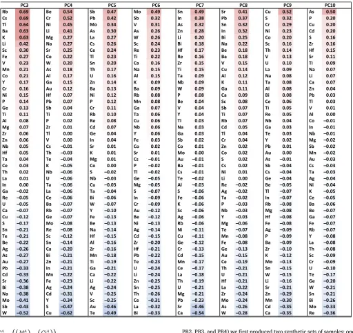
Table of scaled eigenvectors for PC1-PC10, calculated from CLR transformed geochemical data (n= 2726 samples). Values range from 1 (perfect correlation) to −1 (perfect anticorrelation). Each PC has been sorted individually, so that element associations appear at the positive and negative ends of each PC.

Rb 0.69 Be 0.54 Sb 0.47 Mo 0.49 Sn 0.49 Sr 0.41 Cu 0.52 As 0.50

Cs 0.69 Cr 0.52 Pb 0.42 Sb 0.32 In 0.38 Pb 0.37 S 0.32 P 0.20

Tl 0.64 Ni 0.45 Mo 0.34 V 0.31 As 0.32 Sn 0.32 Cr 0.29 Cu 0.20

Ba 0.63 Li 0.41 As 0.30 As 0.26 Zn 0.28 In 0.32 Ni 0.23 Cd 0.20

K 0.63 Mg 0.27 La 0.27 W 0.26 Li 0.20 Bi 0.25 Co 0.20 S 0.16

Li 0.42 Na 0.27 Cs 0.26 Sc 0.24 Bi 0.18 Na 0.22 Sc 0.16 Zr 0.16

Sc 0.30 Sr 0.25 Ce 0.24 Re 0.23 Hf 0.17 Be 0.18 Th 0.14 Hf 0.15

Fe 0.27 Co 0.22 Tl 0.23 Ti 0.22 Re 0.16 Ba 0.18 V 0.13 Sr 0.11

V 0.23 W 0.20 Sn 0.20 Ca 0.16 Zr 0.15 V 0.15 U 0.10 Ti 0.09

Mn 0.21 As 0.18 Th 0.17 Na 0.15 Ti 0.15 Cu 0.14 La 0.09 Na 0.07

Co 0.21 Al 0.17 U 0.16 Al 0.15 Ta 0.09 Al 0.12 Na 0.08 Li 0.07

Y 0.17 Ga 0.15 Zn 0.14 K 0.09 Nb 0.09 K 0.11 Ta 0.08 Ca 0.07

Cr 0.16 Au 0.12 Ba 0.13 Ba 0.09 W 0.09 Ga 0.11 Al 0.08 Zn 0.04

Ni 0.15 Hf 0.07 Ni 0.12 Rb 0.08 P 0.08 Ca 0.09 Bi 0.08 Pb 0.03

P 0.14 Pb 0.07 P 0.12 Mn 0.08 Be 0.04 Sc 0.08 Ce 0.06 Tl 0.03

Ge 0.13 Sb 0.04 Cr 0.11 Ga 0.07 V 0.04 Sb 0.07 Ti 0.05 V 0.01

Ti 0.11 Ti 0.02 Rb 0.10 Ta 0.06 Y 0.04 Ti 0.07 Re 0.05 Al 0.00

Al 0.08 P 0.02 Re 0.08 Cu 0.06 Tl 0.03 Rb 0.07 Nb 0.04 Co –0.01

Mg 0.07 Zr 0.01 Cd 0.07 Nb 0.06 Na 0.03 Cd 0.05 Ga 0.03 In –0.01

Zr 0.06 Tl 0.00 Ge 0.04 Y 0.06 Ga 0.03 Tl 0.04 Te 0.03 Nb –0.01

Zn 0.06 V 0.00 In 0.04 Fe 0.03 Sb 0.02 Cr 0.04 Y 0.02 Mg –0.02

Nb 0.05 Cs –0.01 Sr 0.01 Co 0.02 Co 0.01 Zn 0.02 Pb 0.01 Sb –0.02

Hf 0.05 Th –0.03 K 0.01 Sr 0.01 Mo 0.00 Co 0.02 Au 0.00 Mn –0.02

Ta 0.04 Te –0.04 Mg 0.01 Cs –0.01 Au –0.01 S 0.02 As –0.01 Au –0.03

Ce 0.03 K –0.05 Co 0.00 P –0.02 Ba –0.01 Cs 0.02 Sb –0.04 Cs –0.03

Th 0.02 Nb –0.06 S –0.02 Tl –0.02 Cs –0.01 Ni 0.01 Cs –0.04 Ta –0.03

La 0.01 U –0.06 Nb –0.03 Ge –0.05 Te –0.02 Li 0.00 Ge –0.04 Ag –0.04

In 0.00 Ta –0.06 Cu –0.03 Mg –0.05 Al –0.03 Re –0.02 Be –0.05 Ni –0.04

Ga –0.02 La –0.06 Ta –0.04 S –0.07 S –0.06 Ag –0.02 Tl –0.07 K –0.05

Re –0.05 Ce –0.06 Bi –0.06 In –0.09 Fe –0.06 Ta –0.02 In –0.07 Ce –0.05

U –0.05 Ba –0.07 W –0.07 Cr –0.09 K –0.06 P –0.03 Rb –0.08 Ba –0.06

Ca –0.07 Rb –0.07 Y –0.10 Au –0.12 Sc –0.06 Nb –0.03 Mg –0.08 Be –0.07

Cu –0.12 Ge –0.07 Fe –0.13 Be –0.12 Ag –0.06 Y –0.03 Hf –0.08 Ga –0.07

S –0.17 Mo –0.08 Be –0.13 Ni –0.13 Rb –0.06 Mg –0.06 Fe –0.08 Fe –0.07

Sn –0.21 Re –0.08 Na –0.14 Ag –0.14 Ni –0.11 Te –0.07 Ag –0.09 Rb –0.07

Te –0.21 Sc –0.12 Hf –0.15 Cd –0.15 Cu –0.11 Mn –0.08 P –0.09 Y –0.08

Be –0.22 Sn –0.14 Al –0.16 Zr –0.20 Ge –0.12 Fe –0.08 Ba –0.09 La –0.08

Ag –0.26 Ca –0.20 Zr –0.16 Hf –0.21 Cr –0.13 Ge –0.13 Zr –0.10 Th –0.08

As –0.27 Bi –0.21 Mn –0.18 Pb –0.22 Cd –0.15 Au –0.15 K –0.12 Sc –0.09

Au –0.27 Zn –0.21 Ti –0.19 Te –0.23 Mn –0.17 Ce –0.19 Mo –0.13 Cr –0.09

Pb –0.33 In –0.21 Ga –0.21 U –0.24 Ce –0.17 Th –0.21 Sn –0.15 U –0.10

Cd –0.33 Mn –0.22 Ca –0.22 Li –0.24 La –0.18 U –0.21 W –0.15 Te –0.17

Sr –0.36 Fe –0.23 Li –0.22 Zn –0.25 Th –0.19 Hf –0.21 Li –0.16 Ge –0.20

Bi –0.38 Ag –0.24 Ag –0.24 Sn –0.25 U –0.21 La –0.22 Sr –0.21 W –0.21

Na –0.38 Cd –0.31 V –0.25 Th –0.26 Mg –0.21 Zr –0.24 Zn –0.29 Sn –0.21

Mo –0.41 Y –0.34 Sc –0.25 Ce –0.31 Pb –0.23 Mo –0.24 Mn –0.30 Bi –0.26

Sb –0.43 S –0.47 Au –0.46 La –0.32 Sr –0.46 As –0.26 Cd –0.35 Mo –0.33

W –0.52 Cu –0.62 Te –0.49 Bi –0.33 Ca –0.54 W –0.28 Ca –0.35 Re –0.36

PC9 PC10

represents the alteration subdomain. The two derived matrices are then used to produce a matrix of mass change values which reflect the ori-ginal probability distributions (Ague and van Haren, 1996).

C C C g g g g ( , , M) , , , M

mM M

1 2 1 2

1

… = …

= (2)

whereCM is the concentration of constituent m, and M is the total

number of constituents used to calculate the geometric mean of con-stituent m (gm):

g_m exp N ln(c )

n N n m 1 1 , = = (3)

The AML vectors are denotedAML°_{(protolith suite) andAML}′ (al-tered suite) using Eq.(2), yielding:

AML°=C C1°, 2°, …,CM°, (4)

AML =C C1, 2,…,CM, (5)

Best estimates of mass change are then calculated:

T C C 1, i i = ° (6) C C C C 1, j i i j j = ° ° (7) whereT is the total mass change and j_{is the mass change for mobile} speciesj, calculated using replicate bootstrap analysis.

Immobile elements are identified by constant inter-element ratios for like lithology. Straight lines on scatter plots are conventionally used (Pearce, 1996;Piercey et al., 2002), but the bootstrapped AML matrices provide robust values of C C_i°/ _{i and allow comparison between}

ele-ments. For example, elements with similar proportions ofC Ci°/ i appear as a plateau of values. The geometric mean of immobile element pro-portionsC Ci°/ i, the Geometric Mean Best Estimate (GMBE), represents the immobile-element reference frame from which element addition and depletion are then calculated. A geometric mean is used to calcu-late the GMBE, as literature suggests it provides better results than an arithmetic mean for ratio quantities (Spiegel, 1961).

Next, the GMBE immobile reference frame is used to solve Eq.(7). Five-thousand solutions are generated (as there are 5000 samples is the protolith matrix and 5000 corresponding samples in the altered sample matrix). A geometric mean is used to produce a single mass balance estimate for the alteration domain, and 95% confidence limits are placed about this value. This representation provides an averaged measure of element mass change and a representation of uncertainty arising from geochemical heterogeneity. Confidence limits spanning the 0% mass change line indicate that elements cannot be stated as having had mass gain or loss and cannot be used reliably to quantify or re-present element mass balance. Finally, the geometric mean of values for the representative protolith of each subunit is used to calculate mass balance for each appropriate altered sample in the original dataset. The results are plotted spatially for interpretation in 3-D.

5. Results

5.1. Principal component element patterns

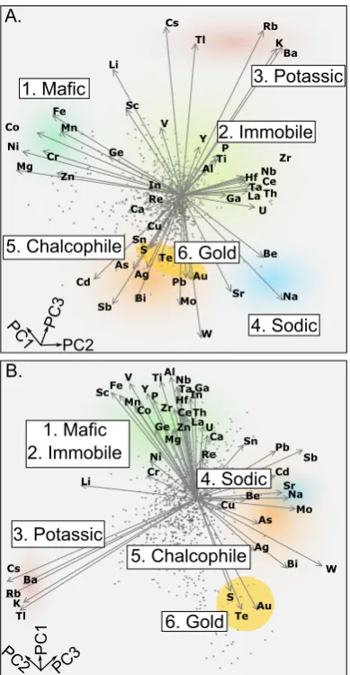
Ten PCs were selected using the change in slope of a scree plot (Fig. 7) and account for 75.9% of data variance for CLR-transformed data (Appendix B. Principal Component Supplement). The relative contributions of elements to each PC are given inTable 2and is co-loured to indicate groups of elements with similar covariance.

Element eigenvectors are plotted in 3-D using PC1—PC3 as axes (Fig. 8). Six groups of elements are defined by similar vector orientation and magnitude: (1) relatively immobile elements, e.g., Ce, Ga, Hf, Nb, La, Ta, Th, and Zr; (2) elements associated with mafic rocks, Ca, Co, Cr, Fe, Ge, Mg, Mn, Ni, and Zn; (3) elements related to potassic alteration: Ba, Cs, K, Rb, and Tl; (4) elements related to sodic alteration: Be, Na, and Sr; (5) chalcophile elements, including Bi and Sb; and (6) Au, Te, and S.

5.2. Immobile element trends

Scatter diagrams were used to examine elements with a sympathetic relationship to Zr (c.f.,Piercey et al., 2002) by plotting Zr against Al, Ga, Hf, Nb, Sc, Ta, Th, V, Y, Cr, and Ni. Zirconium vs. Hf produced the most linear trend (Fig. 9A). These elements were selected to provide the immobile element reference frame, used for all mass balance calcula-tions, as they haveC C_i°/ _{i proportions similar to those of Cr, La, Ce, and}

Ga (Fig. 10).

5.3. Alteration and weathering discrimination

The alkali index (molar Na/Al and K/Al) shows that the highest Au grade samples cluster along the albite-muscovite tie line (Fig. 6A); samples associated with this trend were tagged to represent the altered end-member for mass balance study. Existing work in the St Ives region,

PC1

PC3

PC2

PC1

PC

3

PC2

3. Potassic

5. Chalcophile

2. Immobile

1. Mafic

4. Sodic

A.

B.

6. Gold

3. Potassic

5. Chalcophile

1. Mafic

2. Immobile

4. Sodic

6. Gold

which predates the discovery of Hamlet, suggests that unaltered mafic rocks (including, but not limited to the Paringa Basalt) have alkali index ranges of 0 ≤ K/Al ≤ 0.07 and 0.2 ≤ Na/Al ≤ 0.4 (Prendergast, 2007). We instead selected least-altered boundaries of 0.02 ≤ K/Al ≤ 0.06 and 0.175 ≤ Na/Al ≤ 0.275, which represent the highest point density for unmineralised samples not occurring within the envelope of the Hamlet Shear Zone (Fig. 6A).

Weathering of mafic igneous rocks examined on a ternary plot of Al2O3-CaO-K2O (Nesbitt and Young, 1984), and threshold values of Al2O3/CaO = 0.5 and CaO/K2O = 0.9 were used to isolate least-weathered samples (Fig. 6B). Bounds for both plots were selected based on the highest point density of samples logged to be least-altered and least-weathered. A second filtering to exclude weathered samples was then done. Spatial examination of PC5 and PC6 (Table 2) indicate in-cipient weathering correlated with PC5 > 1 and PC6 > 1. Samples with these values tended to be close to surface, with horizontal con-tinuity, and were omitted from further examination. The resulting number of least-altered and altered sample pairs for PB1 (nine and 30), PB2 (124 and 22), PB3 (141 and 83), and PB4 (31 and 89) exceed the number of pairs demonstrated for bootstrapped mass balance estima-tions in the original study (seven least-altered samples and six altered samples;Ague and van Haren, 1996).

5.4. Mass balance

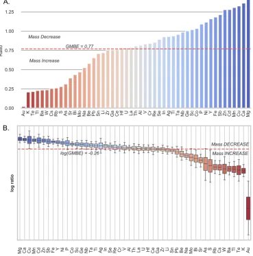
A reference frame defined by Zr and Hf was used for mass balance calculations, for all subunits (Fig. 10). The bootstrapped GMBE re-ference frame values for subunits were each less than one: PB1 = 0.77; PB2 = 0.77; PB3 = 0.99; and PB4 = 0.9. Total mass loss estimates for the subunits are: PB1 = −23%; PB2 = −22%, PB3 = −1%; and PB4 = −10%.

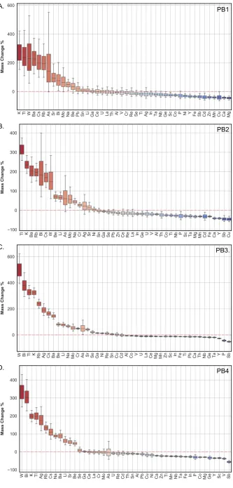
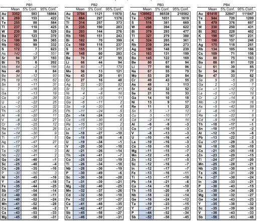
Mass balance estimates for representative alteration subdomains are presented inFig. 11andTable 3. Results indicate that Ba, Bi, Cs, K, Na, Rb and Tl are enriched in samples along the Na-K alteration trend, for all subunits. Mass addition for strongly added elements is on the order of hundreds of percent (Table 3). Note that elements that tend to have very low or LOD values in protolith samples (e.g., Au, Te, and S) yield erroneously high results. Calcium, Cd, Co, Cu, Fe, Ge, Mg, Mn, Sc, Sb, Y, and Zn appear in the depleted region of the mass balance plots for all

subunits. Mass depletion for strongly removed elements is about 40–60% (Table 3).

A sample-by-sample comparison of original data versus mass bal-ance values is presented inFig. 12. Original concentration data (ppm) are plotted against derived mass balance values (%) as probabil-ity–probability (P-P) plots. Raw data have been sorted in ascending order and represent the independent variable and expected probability distribution of samples. Mass balance values on the dependent axis are plotted by corresponding sample number. Deviations from a straight-line straight-linear trend indicate that the mass balance function is not pro-viding a linear rescaling of the original concentration data.

Mass change estimates are calculated for each original sample of Paringa Basalt using results from theAML′_{of corresponding subunits.} Results are shown on long-sections for a selection of these elements in Fig. 13. Potassium (Fig. 13A) suggests multiple orientations for element enrichment defined by smaller clusters of values with ranges up to about 300 m within the shear plane. Sodium (Fig. 13B) shows strongest addition values forming a zone which plunges towards the south-southeast. Calcium (Fig. 13C) depletion appears to correlate to zones of K and Na enrichment. Bismuth (Fig. 13D), like K, displays multiple orientations at short range (less than about 300 m).

6. Discussion

Paringa Basalt samples can be split into six geochemical groups based on PC eigenvector magnitude and direction (Fig. 8). These groups are categorised by electrochemical character and geological observa-tion of the case study area as: (1) elements that are typically immobile; (2) elements generally associated with mafic rocks; (3) elements related to K alteration; (4) elements related to Na alteration; (5) chalcophile elements; and (6) elements strongly associated with Au mineralisation. These groups provide an initial understanding of Paringa Basalt geo-chemistry at Hamlet, as a basis for mass balance calculations and the interpretation of results.

6.1. Discrimination of Paringa Basalt subunits

The Paringa Basalt is fractionated from stratigraphic base to top (Barnes et al., 2012;Walshe et al., 2014), and so must be separated into

Hf (ppm) _Sc

(p

pm

)

K (ppm

)

T

i (

p

pm

)

5.0 7.5

2.5

0 100 200

20000 30000

10000

0 100 200

5000 10000

0 100 200

200 400

0 100 200

Zr (ppm)

Zr (ppm) Zr (ppm)

Zr (ppm) A.

C.

B.

D.

PB4

PB2 PB1 PB3

more geochemically similar subunits to inform mass balance calcula-tions. Elements traditionally used for mafic volcanic rock discrimina-tion include Ti, Zr, Y, Nb, Ce, Ga, and Sc (Cann, 1970; Floyd and Winchester, 1978;Pearce, 1996). However, their use in discriminating Paringa Basalt subunits is nominal because they are not significantly partitioned between the subunits. Previous workers in the Hamlet area used Th-Cr-Ti ternary discrimination plots to separate Paringa Basalt subunits (Walshe et al., 2014), although the Th and Ti axes do not in-fluence the thresholds used (i.e., only Cr separates the respective sub-units). However, a probability plot of CLR transformed Cr (or Ni) allows a straightforward alternative separation of four Paringa Basalt subunits, with Cr content decreasing from north to south (Fig. 4;Fig. 5). The distribution of the subunits compares favourably to previously mapped bedrock geology, where subunits of Paringa Basalt are folded about the Durkin Anticline (Fig. 1).

6.2. Fractionation trends of immobile elements

The classically immobile elements Al, Ce, Ga, Hf, La, Nb, P, Sc, Ta, Th, Ti, V, Y, and Zr (e.g., Pearce and Cann, 1973; Wood, 1980; MacLean, 1990; Jenner, 1996;Rollinson, 2014) group together in PC space of the Hamlet data, indicating a high degree of correlation be-tween these elements despite overprinting alteration and weathering (Table 2andFig. 8). Except for Hf, these elements do not exhibit a strong linear correlation with Zr (e.g.,Fig. 9). While Zr and Hf are also

the most evenly distributed across the case study area (Fig. 4) other immobile elements vary in concentration from north to south. The strong linear correlation between Zr and Hf (Fig. 9) may suggest a si-milar magmatic fractionation history, and/or a mutual host phase such as zircon.

Concentration ratio plots for immobile elements produceC /Ci° i ra-tios around the GMBE, as expected (Fig. 10A and B). This is because ratios should be like those of Zr and Hf, which define the immobile reference frame. However, there is a progression of values defined by the immobile elements, creating a slope of estimates which influence mass balance results. This gradation could indicate either element mobility during alteration or variation within subunits (e.g., due to fractionation). As previously described, the Paringa Basalt is chemically fractionated (Barnes et al., 2012;Walshe et al., 2014), so mass change estimates for immobile elements are spurious, a result of primary gra-dational chemical composition of the basaltic sequence. Therefore, the gradation of mass balance estimates, and corresponding slope on Fig. 11, is interpreted to represent fractionation of immobile elements in basalt host rocks, rather than an alteration effect.

6.3. Geochemical changes associated with Au mineralisation

Previous element mobility studies were undertaken for mafic rocks near Hamlet, in the attempt to understand the implications of element mobility for Au exploration. These studies either infer mass change

A.

B.

A.

B.

C.

D.

PB1

PB2

PB3.

PB4

using univariate concentration data (Eilu and Mikucki, 1996;Walshe et al., 2003), or relative mass change using ratios of univariate data (Prendergast, 2007). Univariate studies suffer from closure issues, ig-noring apparent enrichment/depletion for elements of interest that relate to mobility of other elements. These studies also do not normalise values by rock type, and instead present ranges where upper and lower values are inferred to represent enrichment or depletion, respectively. While studies using element-ratios are not subject to problems related to either closure and normalisation to rock type, they can only present relative enrichment or depletion as unitless values. They also do not consider the heterogeneity of alteration domains or any statistical confidence for interpreted enrichment or depletion of key elements.

To illustrate that mass balance results provide new information, rather than rescaling raw compositional data,Fig. 12shows P-P plots of original sample values versus computed mass change, per sample. Plotted points follow a linear trend, generally indicating that high va-lues in raw data also indicate mass addition, and low raw vava-lues in-dicate mass loss. However, plotted samples are scattered, indicating a non-linear correlation between original concentration and calculated

mass change. The P-P plot of K (Fig. 12) exhibits four separate trends, in order of increasing slope, for PB1–PB4. This relationship helps to il-lustrate an advantage to using rock-normalised mass balance results over compositionally-closed univariate data: calculated K addition is lower for PB1 on average than for PB4, considering identical K ppm values. The P-P plot for Na (Fig. 12) shows two trends for at least PB1 and PB3. This is interpreted to represent two distinct domains of Na mass change. P-P plots for Ca and Bi (Fig. 12) exhibit considerable overlap, suggesting similar mass balance domains present for both elements.

The total mass change is negative, given GMBE values < 1. Mass change estimates (PB1 = −23%; PB2 = −22%, PB3 = −1%; and PB4 = −10%) are inversely proportional to the magnitude of Au, S, and Te enrichment (Table 3).Table 4gives element mass change esti-mates extracted fromTable 3, for samples along the Au mineralisation-related albite-muscovite tie-line (Fig. 6). These values are selected be-cause confidence limits do not span 0% mass change in any subunit, i.e., they are reliable average estimates. The elements associated with mafic rocks (group 1 from PCA;Fig. 8) include Ca, Co, Fe, Ge, Mg, Mn, and Table 3

Mass balance estimates for samples within the Hamlet Na-K alteration trend, calculated as the geometric mean of bootstrapped mass balance results. Warm colours indicate calculated element enrichment, while cool colours indicate element depletion. Mass balance estimates with confidence limits that do not span 0% are given in bold. In contrast, mass balance estimates with confidence limits that span 0%, are marked by italics.

Mean 5% Conf. 95% Conf. Mean 5% Conf. 95% Conf. Mean 5% Conf. 95% Conf. Mean 5% Conf. 95% Conf.

Au 3352 583 16864 Au 3704 1121 11870 Au 138962 86538 218582 Au 61418 32847 111047

K 269 153 422 Te 664 297 1376 Te 1298 1031 1619 Te 944 720 1209

Te 255 88 584 Tl 314 257 373 S 516 381 669 S 479 376 607

Tl 237 110 425 K 235 190 283 W 498 394 622 W 330 250 431

W 230 58 529 Ba 203 144 276 Bi 379 293 477 Bi 302 228 402

Ba 227 123 370 Rb 195 151 243 Tl 327 279 380 K 198 167 231

Cs 199 99 365 Bi 182 70 399 K 324 285 361 Tl 198 157 246

Rb 193 99 332 Cs 169 118 237 Rb 239 204 273 Ag 175 118 251

S 172 7 623 S 155 51 317 Ag 190 148 239 Rb 134 105 166

As 142 –3 551 W 148 60 283 Cs 163 131 199 Cs 109 71 156

Sr 94 37 193 Be 70 47 95 Ba 145 122 169 Na 88 75 103

Bi 75 6 202 Li 66 44 94 Be 80 67 94 Ba 88 61 120

Mo 64 –2 166 As 60 –7 179 Li 77 60 96 Li 61 39 85

Na 49 8 84 Mo 56 13 121 Na 67 55 79 Sr 54 36 77

Be 34 –12 93 Na 43 29 61 Mo 53 29 84 Be 47 33 62

Pb 18 –15 62 Cr 27 16 40 Cr 49 43 55 Se 9 –5 26

Sn 8 –11 31 Ag 22 –20 82 As 48 3 113 Ga 2 –3 7

Li 7 –16 35 Sr 13 –9 41 Sr 42 32 52 Ce –1 –12 12

Ga 1 –13 19 Ni 4 –8 16 Se 21 10 33 La –2 –12 10

Ce 0 –25 39 Sn –2 –13 11 Ga 14 10 18 Cr –2 –14 8

U –2 –22 25 Ga –6 –11 2 Ni 13 9 17 Mo –3 –19 16

La –3 –25 32 Se –9 –20 4 Re 11 1 22 As –5 –42 59

Th –5 –27 25 Pb –11 –24 5 Sn 5 –1 12 U –8 –15 1

Al –6 –20 11 Zn –14 –24 –3 Cu 3 –10 17 Re –9 –22 5

V –8 –32 27 Ce –15 –30 6 Cd –2 –14 10 Cd –9 –19 4

Cr –9 –25 12 Re –15 –29 2 Al –6 –9 –3 Th –10 –17 –1

Re –11 –35 26 La –17 –32 5 Co –7 –10 –3 Sn –10 –17 –2

Se –14 –30 9 In –18 –27 –10 V –8 –13 –3 Al –12 –15 –8

Ti –17 –37 5 Ge –18 –28 –6 U –10 –16 –4 Pb –13 –22 –2

Ag –17 –47 27 U –19 –34 –1 La –10 –16 –3 Cu –17 –29 –5

In –17 –34 4 V –20 –30 –10 Ce –10 –16 –3 Ni –18 –30 –10

Ta –20 –36 3 Al –21 –26 –14 Mg –11 –15 –7 Ca –21 –25 –18

Nb –22 –41 2 Th –24 –41 –7 Mn –12 –15 –9 Zn –23 –29 –15

Ge –24 –40 –1 Co –25 –32 –19 Zn –12 –17 –5 Ti –24 –27 –20

Sc –25 –40 –4 Ti –26 –34 –18 Sc –12 –16 –7 Mn –25 –28 –21

Co –26 –35 –16 Nb –28 –36 –19 In –12 –17 –7 Nb –25 –30 –19

P –30 –50 3 P –30 –49 –6 Fe –13 –16 –11 Ta –26 –31 –20

Ni –31 –45 –16 Sc –30 –38 –20 Ti –13 –17 –10 Fe –27 –30 –24

Y –34 –47 –18 Ta –31 –39 –21 Pb –14 –21 –6 In –28 –33 –21

Fe –35 –44 –25 Mg –32 –40 –25 Ca –14 –18 –10 P –30 –43 –15

Sb –37 –54 –14 Mn –32 –37 –26 Th –15 –20 –9 Co –30 –34 –26

Cd –40 –58 –11 Cd –32 –50 –10 Nb –18 –22 –14 Mg –30 –32 –27

Zn –40 –52 –24 Fe –32 –37 –27 Ge –18 –24 –12 Ge –34 –43 –23

Mn –41 –52 –28 Ca –41 –48 –35 Ta –19 –23 –15 Y –35 –38 –32

Cu –42 –66 –2 Y –42 –47 –37 Y –27 –31 –23 Sc –35 –39 –30

Ca –43 –53 –33 Sb –45 –58 –27 P –44 –52 –34 V –38 –43 –33

Mg –45 –58 –31 Cu –46 –59 –31 Sb –52 –58 –45 Sb –56 –63 –48

Zn, and are consistently depleted in the Au mineralised and altered rocks. The elements Sc and Y (group 2 from PCA;Fig. 8) provide er-roneous results of depletion. This is interpreted as related to fractio-nation of the Paringa Basalt, as discussed above, and are not discussed further. The elements associated with potassic alteration are Ba, Cs, K, Rb, Tl (group 3 from PCA;Fig. 8) and are consistently enriched. Sodic alteration (group 4 from PCA; Fig. 8) is represented only by Na in Table 4, which is enriched. Confidence limits which span 0% for Sr (in PB2;Table 3) and Be (in PB1;Table 3) indicate these elements were omitted as they do not provide reliable average estimates in the sodic group. This effect is interpreted as related to heterogeneity of samples chosen to represent respective protolith sample suites and could pos-sibly be resolved if new suites of protolith samples were selected.

The chalcophile elements (group 5 from PCA; Fig. 8) shown in Table 4are Bi and W (enriched) and Sb (depleted). Finally, elements associated with Au mineralisation (group 5 from PCA;Fig. 8) are Au, S, and Te. These three elements are significantly enriched, although nu-merical estimates are erroneous as respective concentrations are below detection in protolith samples. The values are included mainly to re-present noteworthy addition.

Orogenic Au literature describes the typical mineralisation-asso-ciated metasomatic enrichment of Tl, S, Ag, ( ± As, Sb, W, Te, Se, Mo, Bi, and B; McCuaig and Kerrich, 1998; Eilu and Groves, 2001). In general, this is consistent with Hamlet (Table 3), except in the case of As. The heterogeneity of As is high enough in all subdomains that re-liable mass balance estimates cannot be produced, i.e., estimates have high associated uncertainty (Fig. 11). We note that while our low cal-culated depletion of Sb is not typical for orogenic deposit alteration zones, decoupling between Bi and Sb is described for the nearby Athena deposit (Walshe et al., 2014). Arsenic and Sb enrichment zones in orogenic Au deposits are have been associated with pyrite – pyrrhotite

alteration mineral assemblages (reduced), whereas Bi and Mo enrich-ment zones are associated with an assemblage of pyrite – magnetite (oxidised;Neumayr et al., 2008). Pyrite and pyrrhotite are two hall-mark sulphides in the Au mineralised Hamlet Shear Zone (Fig. 3), while magnetite is rare (Walshe et al., 2003; Walshe et al., 2014). We therefore interpret the observed alteration mineral phases, in con-junction with Sb depletion and Bi addition, to indicate a reduced Au mineralisation event at Hamlet.

6.4. Permeability networks from mass balance estimates

Mass balance trends for key elements K, Na, Ca, and Bi are presented on long sections inFig. 13. Potassium and Na are typically associated with minerals which are spatially coincident with orogenic Au miner-alisation (Groves, 1993). Sodium and K are broadly enriched at Hamlet (Fig. 11;Table 4). Metasomatism during the development of orogenic shear zones has been shown to involve the hydrolysis of feldspar (McCuaig and Kerrich, 1998), interpreted to be expressed at Hamlet as the potassic group (additions of K, Rb, Ba, Cs and Tl) and sodic group (addition of Na). Respectively this corresponds to pervasive biotite developed as an envelope within the shear zone, and to albite asso-ciated with local pervasive alteration, veining, and breccia infill.

There are numerous associations between Na, K, and Au-bearing fluids in orogenic Au deposits, including mafic-hosted examples in the Yilgarn (Ames et al., 1991;Eilu and Mikucki, 1996;Groves et al., 1998; McCuaig and Kerrich, 1998;Nguyen et al., 1998;Knight et al., 2000; Eilu and Groves, 2001). The presence of biotite is important, as fluid-driven mica formation promotes ductile deformation and permeability enhancement of Au-hosting shear zones (Dipple and Ferry, 1992). The regions interpreted to represent enhanced ductile deformation zones are given by enrichment shown inFig. 13A.

K (ppm)

Ca (ppm)

Na (ppm)

Bi (ppm)

K Mass Cha

nge (%)

C

a Mass Cha

nge

(

%)

N

a Mass

Chang

e (%)

Bi Mass Ch

an

ge (%)

Potassium

Sodium

Calcium

Bismuth

A.

B.

C.

D.

Given that albite veining and breccia zones are observed to over-print biotite-altered Paringa Basalt (Fig. 3), we interpret sodic altera-tion (i.e., Na enrichment;Fig. 13B) to overprint potassic alteration (i.e., K enrichment; Fig. 13A). This important relationship represents the facilitation of failure mode transition from ductile to brittle failure, with consequent implications for the nature of fluid flow paths. Albite thus provides a mineralogical control on fault-valve style mineralisa-tion, which has been previously described for other Au deposits in the St Ives camp (Sibson, 1987; Nguyen et al., 1998; Cox, 2005). The pathway of albitisation is interpreted as coincident with Na-enrichment zones (Fig. 13B).

Calcium represents a major mafic-associated element, related to plagioclase in protolith rocks, which is consistently depleted across all subunits. Because Ca is a likely substituted for by K or Na during al-teration, we interpret the pattern shown inFig. 13C to be the inverse of potassic and sodium enrichments. Mapping Ca is thus less useful for understanding pathways of unique metasomatic changes, but poten-tially represents a general fluid flow network.

Finally, Bi (Fig. 13D) is included as a chalcophile element described in the literature as forming a halo around many orogenic Au deposits

(Groves, 1993). Geochemically, Bi is the closest chalcophile element to Au, S, and Te in PC space at Hamlet (Fig. 8). This relationship com-pliments literature which describes Bi as occurring in bismuth-tell-urides associated with Au (Ciobanu et al., 2005;Goldfarb et al., 2005; Tooth et al., 2011).

6.5. Mass balance models as a proxy for Au mineralisation

Fig. 14presents mass balance data for Bi in 3-D. While contoured regions are used to interpret spatial continuity orientations of Bi mass balance inFig. 13D, individual points are used inFig. 14to provide an interpretation of possible fluid flow network segments. The trend-plunge of segments are constrained by geostatistical interpolation around Bi enrichment (parameters are given in Appendix D. Inter-polation Parameters). These interpolated wireframes of Bi addition are coincident with zones of Au mineralisation given by block model esti-mation (Fig. 14).

Four trends of Bi addition are interpreted using strongest Bi addi-tion: steeply dipping plunges to the northeast and south-southeast, and shallowly dipping plunges to the north-northeast and southeast

A.

B.

Strong addition

Weak addition

Weak depletion

Strong depletion

Potassium

Sodium

Classified whole-rock ICP

geochemical samples:

C.

Calcium

D.

Bismuth

250m

PB1

PB2

PB3

PB4

PB1

PB2

PB3

PB4

PB1

PB2

PB3

PB4

PB1

PB2

PB3

PB4