Design, Analysis, And Computational Methods For Engineering Synthetic Biological Networks

(1)

Engineering Synthetic Biological Networks

Thesis by

Ania-Ariadna Baetica

In Partial Fulfillment of the Requirements for the degree of

Doctor of Philosophy

CALIFORNIA INSTITUTE OF TECHNOLOGY Pasadena, California

2018

(2)

Ania-Ariadna Baetica ORCID: 0000-0003-0421-8181

(3)

ACKNOWLEDGEMENTS

First, I would like to acknowledge my committee members for their valuable feedback and helpful comments. I would like to thank my adviser Richard Murray for being endlessly supportive and for giving the best advice. I pretty much struck gold with Richard and I genuinely do not think I could have chosen a better adviser. He provided the correct combination of space, support, and advice to help me grow. He also exposed me to opportunities and challenges that felt outside of my reach at the time, but they served to propel me forward. Just being in the same room as Richard and watching him interact with people is an invaluable lesson in leadership. I would also like to thank him for pushing me to give every opportunity a shot because who knows you might just start that thesis or get that position. To summarize, I would like to thank Richard for teaching me how to be a leader and how to solve all of my problems in at least twelve different ways.

I would also like to thank John Doyle for being an incredibly inspiring scientist and for thinking so far ahead of the curve. John has a unique and unparalleled understanding of science that has influenced how we all think. He has reinvented and redefined what it means to be an engineer in science and, in particular, in biology. It probably took me about five years to begin to understand John’s thinking, but I greatly benefited from his comments and feedback. I am also thankful to Brian Munsky for creating an environment of opportunities at the q-bio summer school and for being very patient and meticulous. I am thankful to Niles Pierce for carefully listening to my ideas and for giving me his opinions and feedback.

(4)

collaborator and a great storyteller. I am grateful for the chance to have had mutual mentorship relationships with Cindy Ren, Reed McCardell, and Fangzhou Xiao. Like all members of the Murray lab, I am grateful to Enoch Yeung, Victoria Hsiao, Anu Thurbagere, and Shaobin Guo for being people to look up to.

My gratitude also goes out to my friends for being there for me during graduate school. I want to thank Qiaochu Yuan for laughing with me, often at me, and for always giving me her couch to crash on. I want to thank Armeen Taeb for being a great friend, Tegan Brennan for being lovely and chill, and Yoke Peng Leong for being patient and supportive. I have greatly enjoyed dinners and stories at Settebello with my friends Armeen and Ioannis Filippidis. I would also like to thank my friends Yorie Nakahira, Yong Sheng Soh, Corina Panda, Tony Bartolotta, Monica and Laura Nastasescu, Bogdan Stoica, Mickey Wang, Andrey Shur, Leo Green, Michaelle Mayalu, and Niangjun Chen. Many thanks go to Monica Nolasco, Maria Lopez, Nikki Fauntleroy, and Sydney Garstang for helping out so many times and for organizing the department tea. Many thanks to Carmen Nemer-Sirois for helping Thomas and I with our wedding. I cannot give enough thanks to Jenny Butler for always being there for me and for guiding me in the right direction. Jenny has changed the course of my life and I will always benefit from having met her. I am thankful to my family for inspiring me to work hard for my dreams and for believing that I could achieve anything and everything. I would like to thank my grandfather Tudor for his unquestionable support and patience and my grandmother Ioana for her spirit, passion, and confidence in me. Additionally, I would like to thank my mother Georgeta for being so hard working and my father Cornel for being my first teacher.

(5)

ABSTRACT

This thesis advances our understanding of three important aspects of biological sys-tems engineering: analysis, design, and computational methods. First, biological circuit design is necessary to engineer biological systems that behave consistently and follow our design specifications. We contribute by formulating and solving novel problems in stochastic biological circuit design. Second, computational methods for solving biological systems are often limited by the nonlinearity and high di-mensionality of the system’s dynamics. This problem is particularly extreme for the parameter identification of stochastic, nonlinear systems. Thus, we develop a method for parameter identification that relies on data-driven stochastic model reduction. Finally, biological system analysis encompasses understanding the stability, perfor-mance, and robustness of these systems, which is critical for their implementation. We analyze a sequestration feedback motif for implementing biological control. First, we discuss biological circuit design for the stationary and the transient distri-butional responses of stochastic biochemical systems. Noise is often indispensable to key cellular activities, such as gene expression, necessitating the use of stochastic models to capture their dynamics. The chemical master equation is a commonly used stochastic model that describes how the probability distribution of a chemi-cally reacting system varies with time. Here we design the distributional response of these stochastic models by formulating and solving it as a constrained optimization problem.

Second, we analyze the stability and the performance of a biological controller implemented by a sequestration feedback network motif. Sequestration feedback networks have been implemented in synthetic biology using an array of biological parts. However, their properties of stability and performance are poorly understood. We provide insight into the stability and performance of sequestration feedback net-works. Additionally, we provide guidelines for the implementation of sequestration feedback networks.

(6)

(7)

PUBLISHED CONTENT AND CONTRIBUTIONS

[Men+17] X Flora Meng, Ania-Ariadna Baetica, et al. “Recursively constructing analytic expressions for equilibrium distributions of stochastic bio-chemical reaction networks”. In:Journal of The Royal Society Inter-face14.130 (2017), p. 20170157. doi:10.1098/rsif.2017.0157. AAB designed the stationary behavior of the two-component tran-scriptional network using its analytical solution. AAB conceived the project and participated in writing the manuscript.

[Ols+17] Noah Olsman, Ania-Ariadna Baetica, et al. “Hard limits and perfor-mance tradeoffs in a class of sequestration feedback systems”. In: bioRxiv(2017), p. 222042. doi:10.1101/222042.

AAB determined the stability and the performance of the seques-tration feedback controller with controller species degradation. AAB conceived the project and participated in writing the manuscript. [Ren+17] Xinying Ren, Ania-Ariadna Baetica, et al. “Population regulation in

microbial consortia using dual feedback control”. In:bioRxiv(2017). doi:10.1101/120253.

AAB analyzed the biological controller implemented by the chemical reaction network. AAB participated in the writing of the manuscript. [Bae+16] Ania-Ariadna Baetica, Thomas A Catanach, et al. “A Bayesian ap-proach to inferring chemical signal timing and amplitude in a tem-poral logic gate using the cell population distributional response”. In: bioRxiv(2016). doi:10.1101/087379.

AAB adapted and implemented the stochastic temporal logic gate model. AAB formulated the research question and participated in writing the manuscript.

[Bae+15] Ania-Ariadna Baetica, Ye Yuan, et al. “A stochastic framework for the design of transient and steady state behavior of biochemical reaction networks”. In:2015 IEEE 54th Annual Conference on Decision and Control (CDC). IEEE. 2015, pp. 3199–3205. doi: 10 . 1109 / CDC . 2015.7402699.

(8)

Appendix A: Theorem proofs for the design of stochastic biochemical reaction networks . . . 93 Appendix B: Theorem proofs for Sequestration Feedback Networks . . . 98 B.1 Sequestration feedback networks with no controller species degradation 98 B.2 Sequestration feedback networks with controller species degradation 99 B.3 The critical controller species degradation rate . . . 99 B.4 Stability analysis of the sequestration feedback network with

(10)

LIST OF ILLUSTRATIONS

Number Page

1.1 The Markov state space associated with the chemical master equation 5 1.2 The time-varying probability distributions of biochemical speciesS2

computed using the chemical master equation . . . 7 1.3 The finite state projection method . . . 8 1.4 The engineering design cycle as a methodical approach to problem

solving . . . 9 1.5 Reference tracking . . . 11 2.1 Schematic representation of the fluorescence of anE. colicell

popu-lation that carries the genetic toggle switch . . . 18 2.2 A biological system of two interconnected transcriptional

compo-nents [GD12] . . . 22 2.3 Designing the global maximum of the joint stationary distribution

of the complex species and the transcription factor species using its analytical form . . . 24 2.4 Solution to the design problem for a protein production-degradation

reaction network . . . 29 2.5 Solution to the design problem for the Schlögl reaction network with

unimodal transient constraints . . . 31 2.6 Solution to the design problem for the Schlögl reaction network with

bimodal transient constraints . . . 32 2.7 Solution to the design problem for the Schlögl reaction network with

bimodal transient constraints . . . 33 2.8 The biological circuit diagram for the genetic toggle switch adapted

from [GCC00] . . . 33 2.9 Solution to the design problem for the genetic toggle switch with

bimodal transient constraints . . . 35 3.1 Sequestration feedback network diagram . . . 38 3.2 The strength of the sequestration reaction . . . 43 3.3 The sequestration feedback network’s controller and process networks 45 3.4 The stability of the sequestration feedback network with varying

(11)

3.5 The critical controller species degradation rate . . . 51 3.6 The tradeoff between small steady state error and large stability margin 53 3.7 Guidelines for designing sequestration controllers . . . 57 4.1 Bursting gene expression diagram . . . 67 4.2 Radial basis function interpolation of simulated single-cell data for

the bursting gene model . . . 68 4.3 Likelihood functions of the FSP and of the RBF-FSP for two

param-eter combinations of the bursting gene expression model . . . 69 4.4 The parameters of the bursting gene model, as identified using a

version of the adaptive Metropolis-Hastings algorithm . . . 70 4.5 Radial basis function interpolation of simulated single-cell data for

the genetic toggle switch in [GCC00] . . . 71 4.6 The parameter distributions obtained from the Metropolis-Hastings

algorithm for the genetic toggle switch with the FSP and the RBF-FSP models . . . 73 A.1 Solution to the design problem for a protein production-degradation

reaction network . . . 96 A.2 A piece-wise projection operator that constrains a corresponding

transient distribution to be bimodal . . . 97 B.1 The steady state error as a function of the controller degradation rate. 100 B.2 A sequestration feedback network with a simplified process . . . 103 B.3 A sequestration feedback network with two process species . . . 112 B.4 The sequestration feedback network with the controller species

im-plemented with transcriptional parts and the process species imple-mented with protein parts . . . 115 B.5 The stability of the sequestration feedback network with different

process species degradation rate and strong sequestration feedback . . 116 C.1 The probability distributions generated by the parameters identified

using the two projections and the simulated data for the bursting gene model . . . 120 C.2 The joint distributions of the parameters identified using the

Metropo-lis Hastings algorithm for the bursting gene model. . . 121 C.3 Illustration of the genetic toggle switch, adapted to the example in

Section 4.5 . . . 121 C.4 The probability distributions generated by the parameters identified

(12)

LIST OF TABLES

Number Page

3.1 The degradation rates of biological parts that could be used to build sequestration controllers . . . 44 4.1 The maximum values of the RNA transcription rate and of the

tran-scription factor unbinding rate for the FSP and the RBF-FSP reduc-tions of the gene bursting model . . . 70 4.2 The parameters of the genetic toggle switch identified by the

Metropolis-Hastings algorithm . . . 72 B.1 The parameters used for the simulation in Figure 3.5 . . . 101 B.2 The units of the biochemical species and rates in the sequestration

feedback network . . . 112 B.3 The units of the biochemical species and rates in the scaled

seques-tration feedback network . . . 113 B.4 The half-lives of biological parts that could be used to build

seques-tration controllers . . . 113 B.5 The on-rate of the sequestration reaction. . . 114 B.6 The parameters used for a simulation with controller species

(13)

C h a p t e r 1

INTRODUCTION

1.1 A brief introduction to synthetic biology

The field of synthetic biology engineers novel organisms, devices and systems for the purposes of improving industrial processes [Nar+16; Hem+10; SWS08; CG10;DKM10], discovering the principles of biological systems [GCC00;EL00; GHM14], and performing computation and compact information storage [Thu17; Hsi+16]. In synthetic biology, we build systems inspired by natural biological sys-tems, but we do not restrict ourselves to parts and designs already available. The numerous applications of synthetic biology include industrial fermentation [GM12], waste detection [Sim+08], biosensors development [Hsi+16], diagnostics detec-tion [Par+14], materials producdetec-tion [Ngu+15;CG08], novel protein design [Arn98], information storage [Thu17], and biological computation [Moo+12]. Since synthetic biology is a relatively novel field, its applications and capabilities are still expanding. However, synthetic systems have a unique set of challenges and limitations. A goal of synthetic biology has been to engineer reliable, robust circuits composed of standardized parts that can easily be combined together [CLE08; Ark08; Kwo10; KC10;QD17]. Nevertheless, it has been demonstrated that synthetic circuits depend on their biological implementation [DM15; Yeu+14; Yeu+17]. Slight differences in the circuit’s tuning, implementation in a different model organism [KZH09], or different experimental conditions can all cause synthetic circuits to cease func-tioning [GMB16; PW09]. This limits the modularity of synthetic circuits and the engineering of larger circuits. Additionally, synthetic systems are often subjected to strict resource limits that result in limited functionality and in competition with the host organism [QMD17; GD14]. Furthermore, synthetic systems oftentimes rely on transcriptional parts, which results in slower response timescales than natural biological systems, particularly when the product is a protein [Ngu+15].

(14)

1.2 Biochemical kinetics

Notation

Let_Zand_Rbe the integer set and the real set, respectively.

Letn ≥ 1 be an integer. LetP∈ [0,1]nbe then-dimensional probability vector set. Forp= (p1, . . . ,pn) ∈ P, it must be thatpi ≥ 0 andÍ_in₌₁pi =1. We denote by AT

the transpose of the matrixA.

Let the symbols A−B and A : B represent the binding of two molecules A and B into a complex.

For our synthetic circuit diagrams, we adhere to the conventions of the Synthetic biology open language [Gal+12].

Deterministic chemical kinetics

Our assumptions for deterministic chemical kinetics are that they employ either unimolecular or bimolecular reactions and mass action kinetics, unless otherwise specified. The law of mass action states that the rate of a chemical reaction is proportional to the product of the concentrations of the reactants. We consider a chemically reacting network withN species{S1, . . . ,SN}andM chemical reactions

{R1, . . . ,RM}. Then we can express the mass action kinetics as

dx

dt =Wv(t), (1.1)

wherexis the concentration of the chemical species,t ∈_R_≥0is the time,W ∈_RN×M is the stoichiometry matrix, andv(x) ∈ _RM×1 _{is the reaction flux vector. Each row}

of the flux vector v(x) corresponds to the rate at which a given reaction occurs. The columns of the stoichiometry matrix denote the changes in concentration of the chemical species. We describe the stoichiometry matrix in more detail in Section1.2. Example 1. We derive the deterministic model of an example biochemical reaction network. Let the following chemically reacting system with speciesS1be described

by the two reactions:

S₁−−−₎₋₋₋k2*

k1

∅. (1.2)

Here speciesS1can represent mRNA or protein that is being created at rate k1and

(15)

flux vector isv(t)= (k1,k2S1(t))T. Therefore, the mass action kinetics are given by:

dS1(t)

dt = k1−k2S1(t). (1.3)

In addition to mass action kinetics, we employ Hill kinetics to describe the coop-erative binding of ligands to a macromolecule [Hil10]. Coopcoop-erative binding means that the binding of a ligand to a macromolecule is enhanced by the presence of other ligands that are already bound to the macromolecule. Moreover, the Hill co-efficient quantifies the degree of cooperativity between ligand binding sites. In the famous example of theO2molecule binding haemoglobin in red blood cells to form

oxyhaemoglobin and be transported to body tissues, the Hill equation models these saturated binding dynamics. At low oxygen concentrations, there is haemoglobin in the blood and almost no oxyhaemoglobin in body tissues. However, at high oxygen concentration, there is almost no haemoglobin in the blood and lots of oxyhaemoglobin in body tissues. Each haemoglobin molecule can bind up to four

O2 ligands, which would suggest a Hill coefficient of four. In practice, the Hill

coefficient is 2.8 due to the limitations of the Hill modeling framework and due to the haemoglobin molecule existing in multiple states. The Hill equation can be represented as

Hb+4 O₂−−−)k−−−a*

k_d Hb−4 O2, (1.4)

wherekaandkdare the association and disassociation constants, Hb is the haemoglobin

molecule, and Hb−4 O₂is the oxyhaemoglobin molecule. We let the dissociation constantKd be the ratio of kd andka. Then the concentration of oxyhaemoglobin,

[Hb−4 O₂], can be computed as:

fHill(O₂)=

[O₂]4

Kd+[O₂]4

. (1.5)

In this thesis, we employ the Hill function to model the transcription of a gene product when its DNA is regulated by multiple transcription factors such as activators and repressors [Alo06]. It is assumed that the transcription factors bind DNA cooperatively. Let A and R be the activator and the repressor, respectively, with basal expression levels ofA0andR0and dissociation constantsKAandKR. LetnHill

(16)

Hill functions associated with the activator, f_Hilla (A), and the repressor, f_Hillr (R), are as follows:

f_Hilla (A)=

α A KA

1+

A KA

nHill + A0, f r

Hill(R)=

α

1+

R KR

nHill +R0. (1.6)

For more details, we refer the reader to [Alo06] and [DM15].

Stochastic modeling with the chemical master equation

Stochasticity in biochemical systems comes from the thermodynamics of molecu-lar reactions [DM15]. We consider a chemically reacting network with N species {S1, . . . ,SN}andMmonomolecular or bimolecular chemical reactions{R1, . . . ,RM},

as in [Gil07]. The dynamical state of the system at timet ≥ 0 is described by the state vectorx(t)=(x1(t), . . . ,xN(t)), where xi(t)is the integer population of species

Si at time t for all 1 ≤ i ≤ N. The M chemical reactions change the state of the

system according to the propensity function associated with each reaction.

The chemical master equation (CME) describes how stochastically reacting chemical species behave in a well-stirred solution at thermal equilibrium in a fixed, finite volume [Gil07]. The chemical kinetics of the N reacting molecular species are modeled as a discrete-state, continuous-time Markov process. A state x of the Markov process is a combination of counts of the N reacting molecular species, while the distribution state vectorp(x,t)denotes the probability that the system will be in state x at time t. The CME gives the time evolution law for p(x,t) as the ordinary differential equation

∂p

∂t(x,t)=

M

Õ

j=1

(aj(x−ξj)p(x−ξj,t) −aj(x)p(x,t)), (1.7)

whereξj is the jt h column of the stoichiometry matrix and aj is the jt h propensity

function associated with the chemical reaction network [Gil00].

More compactly, the CME can be written as an ordinary differential equation

dp

dt(x,t)=H(c)p(x,t), (1.8)

where c = (c1, . . . ,cK) are the K rate reaction parameters of the M chemical

(17)

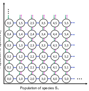
0,0 1,0 2,0 3,0 4,0 5,0 0,1 1,1 2,1 3,1 4,1 5,1 0,2 1,2 2,2 3,2 4,2 5,2 0,3 1,3 2,3 3,3 4,3 5,3 0,4 1,4 2,4 3,4 4,4 5,4 0,5 1,5 2,5 3,5 4,5 5,5

Population of species S1

P

op

ul

at

io

n

of

sp

eci

es

S2

…

[image:17.612.162.463.96.406.2]

…

Figure 1.1: The Markov state space associated with the chemical master equa-tion. We represent the two-dimensional, infinite Markov state space of a toy bio-chemical reaction network with species S1 andS2 (N = 2) and chemical reactions

given in equations (1.9)-(1.11) (M = 4). The state x of the system is a two-dimensional vector whose values are all possible combinations of counts of species

S1andS2; therefore, x is infinite. The arrows represent the possible transitions

be-tween states, according to the four chemical reactions in equations (1.9)-(1.11) and under the assumption that state counts must be at least zero. The state transitions corresponding to the two chemical reactions in equation (1.9) are drawn as blue bidirectional arrows since species S1 can either be created or degraded. The state

transitions for the chemical reaction in equation (1.10) are drawn as green arrows pointing downwards to represent the degradation of species S2. Finally, the state

transitions for the chemical reaction in equation (1.11) are drawn as fuchsia arrows to represent the creation of species S2; since species S2 cannot be created in the

absence of species S1, the states with zero counts of S1 do not have arrows. The

probability of the transition between two states is given by the propensity function

aj(x), associated to the jt h chemical reaction in the system and dependent on the

(18)

Example 2. We derive the chemical master equation model for an example biochem-ical reaction network. Let the following chembiochem-ically reacting system with speciesS1

andS2be described by the set of reactions:

S₁−−−₎k₋₋₋1*

k2

∅, (1.9)

S₂−−−→ ∅k3 , (1.10)

S₁−−−→k4 S₁+S₂. (1.11)

Here speciesS1can represent mRNA and speciesS2can represent protein.

Then the propensity functions associated with the four chemical reactions are

a1(x1,x2) = k1x1, a2(x1,x2) = k2, a3(x1,x2)= k3x2, a4(x1,x2) = k4and the

state-change vectors areξ1= (−1,0)T, ξ2= (1,0)T, ξ3 =(0,−1)T, ξ4 =(0,1)T, where x1is

the number of molecules of speciesS1andx2is the number of molecules of species

S2.

Therefore the CME associated to this system is as follows:

∂p ∂t " x1 x2 # ,t !

= k1(x1+1)p

"

x1+1

x2

# ,t

!

+k2p

"

x1−1

x2

# ,t

!

+ (1.12)

+k3(x2+1)p

"

x1

x2+1

# ,t

!

+k4p

"

x1

x2−1

# ,t

!

− (1.13)

− (k1x1+k2+k3x2+k4)p

" x1 x2 # ,t ! , (1.14)

for x1,x2 ∈Z, x1 >0, x2 > 0.

A simulation of this system is illustrated in Figure1.2.

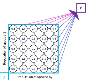
The finite state projection algorithm

The finite state projection approach (FSP) [MK06] truncates the state space of chemical master equation and collects the probability mass that leaves the truncated region in a sink state, g(t). The CME state space is split into two complete and disjoint sets, indexed byJ andJ0, such that the CME becomes

d dt

"

pJ

pJ0

#

=

"

HJ J HJ J0 HJ0_J H_J0_J0

# "

pJ

pJ0

#

(1.15)

(19)

Figure 1.2: The time-varying probability distributions of biochemical species

S2 computed using the chemical master equation. For chemical reactions in

equations (1.9)-(1.11) with reaction rate parameter values k1 = k4 = 100, k2 = 1,

k3 = 0.1, we ran 1000 simulations for 100 seconds each to generate the set of

probability distributions of the biochemical speciesS2. We subsequently fit Gaussian

distributions to the probability distributions from the CME for ease of interpretation.

the sink state after exitingJ). This new master equation is known as the finite state projection, and can be written as

d dt

"

pFSP_J

g(t)

#

=

"

HJ J 0

−1THJ J 0

# "

pFSP_J

g(t)

#

(1.16)

The FSP approximation is guaranteed to be a lower bound on the true solution,

"

pFSP_J

0

#

≤

"

pJ

pJ0

#

for allt > 0, (1.17)

and it yields an exact error in the approximation,

"

pFSP_J

0

#

−

"

pJ

pJ0

# 1

= g(t), (1.18)

where |v|1 denotes the norm-1 of the vector. Proofs of these results are available

in [MK06;MK07].

(20)

0,0 1,0 2,0 3,0 4,0

0,1 1,1 2,1 3,1 4,1

0,2 1,2 2,2 3,2 4,2

0,3 1,3 2,3 3,3 4,3

0,4 1,4 2,4 3,4 4,4

Population of species S1

P

op

ul

at

io

n

of

sp

eci

es

S2

J

[image:20.612.160.468.62.337.2]

J’

Figure 1.3: The finite state projection method. For chemical reactions in1.9-1.11, we truncate the infinite state space of the associated CME to a finite state space J

(blue rectangle). The setJ0(purple) collects all the remaining probability and once it enters it, probability does not escape it. The finite state spaceJ is illustrated and is often chosen to be a hyperrectangle, but it can have any shape.

The matrix exponential solution to the chemical master equation

Using the finite state projection algorithm in [MK06], we truncate the Markov state space of the chemical master equation. Thus, we consider only a finite number of statesSin each species of a biochemical reaction network.

In Chapters2 and 4, we assume that the propensity functions aj are linear in the

reaction rate variables for all 1 ≤ j ≤ M. Then the Markov transition matrix H(c) is finite and we can represent it as the following sum:

H(c)=ΣM_j₌₁cjHj, (1.19)

where each matrix Hj corresponds to chemical reaction Rj for 1 ≤ j ≤ M. The

matricesHj are sparse and of sizeSN ×SN.

Hence, equation (1.8) is equivalent to

dp

dt(x,t)=Σ

M

(21)

which implies linearity with respect to the reaction ratesc1, . . . ,cM.

Therefore, the solution to equation (1.20) is given by

p(x,t)= eΣMj=1cjHjt_p₍_x,₀₎. _(1.21)

Remark 1. The exponential operator eΣMj=1cjHjt _{is not separable into the product}

ÎM

j=1e

cjHjt_{, unless the matrices}_H

1, . . . ,HM commute pair-wise. This is not usually

the case, unless all the M reactions in the system are monomolecular and all the matrices are diagonal [JH07]. For bimolecular reactions, the corresponding matrices do not generally commute.

1.3 Control theoretical concepts for synthetic biology

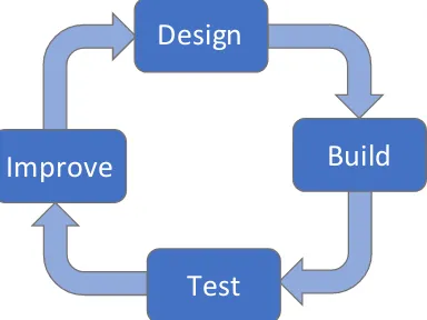
In this section, we introduce the engineering perspective on the development of synthetic circuits. The engineering design cycle described in Figure 1.4 can be employed in synthetic biology; this approach has previously been used in me-chanical and electrical engineering [AM08]. According to the engineering design cycle, synthetic circuits can be iteratively designed, built, tested, and improved until they achieve the desired performance standards. This thesis contributes to design through the performance specifications in Chapter2, to testing through the perfor-mance properties in Chapter3, and to improvement through the recommendations in Chapter3. The computational methods in Chapter4contribute to both the design of synthetic circuits and to the evaluation of their performance.

Design

Build

Improve

[image:21.612.213.405.471.615.2]

Test

(22)

A common method to improve the performance of mechanical and electrical sys-tems is feedback control. The principle of feedback control is to measure the error between the desired and the current performance of a circuit and to take correc-tive action as necessary [AM08]. Feedback is ubiquitous in endogenous biological systems, where it serves to regulate their behavior. Examples of feedback control found in endogenous systems include the regulation of body temperature [Wer10], of circadian rhythms [Rus+07], of calcium [EGK02], and of glycolysis [CBD11]. Analogously, we are developing feedback control to regulate the behavior of syn-thetic systems and to ensure that they behave robustly.

Feedback control provides undeniable benefits to biological, mechanical, and elec-trical systems. The foremost benefit is robustness to uncertainty; should the system undergo a change such an external disturbance, feedback corrects this change and ensures the system retains good performance properties. Additionally, feedback can stabilize and speedup an unstable or slow process. Yet, feedback control also comes with several drawbacks. Feedback can inadvertently amplify noise inside a system and it can also exacerbate instability if poorly designed. For a more detailed understanding of feedback control, particularly in the context of synthetic biology, see the textbooks [DM15;AM08].

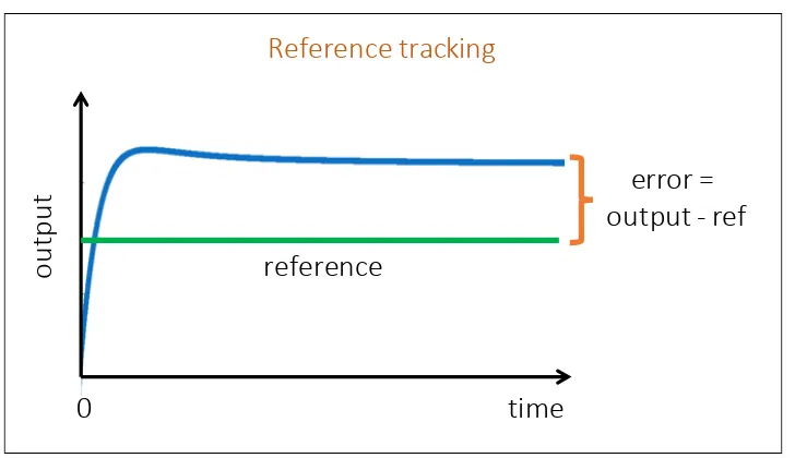
In Figure1.5, we introduce the reference tracking setup that we use for biological feedback control throughout Chapter 3. The goal of reference tracking is for a system’s output to track a pre-determined reference signal. The error signal measures the difference between the output and the reference as a function of time. When the error converges to a real valueessas a function of time, the system is deemed stable and its steady state value is ess. Conversely, if there is no value ess ∈ _R that the error converges to, then the system is unstable. The magnitude of the steady state erroress is a performance measure of the system in Chapter3; a common goal is to ensure a small magnitude ofess.

(23)

ou

tp

ut

time

reference

0

[image:23.612.126.490.66.276.2]

error =

output - ref

Reference tracking

Figure 1.5: Reference tracking. The error measures the difference between the output of the process and the reference specified by the user. When the error converges to a real value as a function of time, we refer to it as the steady state error. Additionally, the closed loop system is deemed stable. If the error does not converge to a real value as a function of time, then the closed loop system is unstable. The magnitude of the steady state error will be used as a performance measure in Chapter3for the closed loop system. The reference can vary as a function of time.

aims to anticipate future errors; however, it can also amplify high frequency process noise. In practice, proportional and integral control are used ubiquitously to regulate mechanical and electrical systems [AM08].

There are multiple differences between implementing feedback control in engineered systems and in biological systems. One difference is that the reference signal may not be an explicit signal, but rather the result of other biochemical dynamics; additionally, when implemented by chemical reactions (such as the constitutive production of a biochemical species in Chapter3), the reference can be dependent on temperature and pH, subjected to disturbances itself, or coupled to other dynamics external to the circuit. The differences between engineered and biological systems have created questions about the performance of synthetic circuits. We discuss this topic in Chapter3and we also further address the differences between engineered and biological feedback systems.

1.4 Contribution overview

(24)

equation. When available [JH07;GLO05;GSN12;SS08;GD12;ACK10], analytic solutions to the CME can greatly simplify the design of distributional responses of biochemical networks. Nonetheless, analytic solutions are challenging to find due to the high dimensionality of the Markov space underlying the CME model, which scales exponentially with the number of species in the network. In Menget al. [Men+17], we have described recursive algorithms for gluing together simple Markov state spaces at one or two vertices to derive analytic stationary solutions to CME models with large Markov spaces [MHK14; MP15]. Using a recursive algorithm, we have derived the analytic stationary solution to the transcriptional network example in [GD12]. In Chapter 2, we illustrate how to use this analytic stationary solution to design the transcriptional network’s stationary behavior. We employ this transcriptional network example to illustrate how designing the stochas-tic behavior of biochemical reaction networks is simplified by the availability of an analytic solution to the CME model.

Subsequently, we propose a general framework for the design of stochastic behaviors of biochemical reaction networks for which analytical solutions to their CME mod-els may not be available [Bae+15]. Design specifications for distributions include specifying their modality, the locations of their modes, and their rate of conver-gence to stationarity [MG09]. We formulate these specifications as constraints in an optimization program that finds the reaction rate values that achieve in the de-sired distributional design. We apply our stochastic design framework to examples of biochemical reaction networks such as a protein production-degradation net-work [DM15], the Schlögl model [Gil91; Gun+05], and the genetic toggle switch model [GCC00] to illustrate its strengths and limitations.

The content of Chapter2has been published in [Bae+15] and [Men+17]. Contribution summary in [Men+17]:

• Designed the behavior of a two-component transcription network using the analytic form of its stationary distribution.

Contribution summary in [Bae+15]:

(25)

• Mathematically described distributional design specifications of modality, location of modes, and convergence to stationarity.

• Formulated and solved the distributional design problem as an optimization problem constrained by the design specifications.

The development of synthetic biological controllers for microbes and fungi can help address problems in human health through scheduled oral probiotic delivery, in industrial fermentation through the improved commercial production of enzymes, and in waste recycling through the improved treatment of sewage effluent for drinking water. In Chapter3, we use methods from control theory to determine the properties of stability and performance of biological controllers implemented by sequestration feedback. Using these metrics of stability and performance, we provide guidelines for the implementation of robust synthetic biological controllers.

First, we introduce biological control using sequestration feedback and we demon-strate that the controller species’ sequestration binding strength, the process species’ degradation rates, and the controller species’ degradation rates affect their stability and performance properties. We then derive an analytical criterion for stability and we tune the stability margin by increasing either the process or the controller species degradation rates.

Second, we determine the performance of sequestration feedback networks when the controller species are degraded and diluted due to cell division or fungi budding. It has been demonstrated that a stable sequestration feedback controller with no controller species degradation implements perfect adaptation, which provides these biological controllers with robustness and zero steady state error [BGK16]. More-over, we derive performance results that consider the controller species degradation and dilution and we provide robust implementation choices that guarantee a small steady state error.

Finally, we describe a tradeoff between the stability and the performance of seques-tration feedback networks. Additionally, we give guidelines for building sequestra-tion feedback networks with respect to this tradeoff.

The content of Chapter3has been published in [Ols+17] and [Ren+17]. Contribution summary to [Ols+17]:

(26)

• Determined the stability and the performance of the sequestration feedback controller with controller species degradation.

• Provided guidelines for the implementation of sequestration feedback net-works.

Contribution summary to [Ren+17]:

• Analyzed the cell population controllers implemented using sequestration feedback networks.

In Chapter4, we introduce a novel method for parameter identification of stochas-tic biochemical reaction networks. Probabilisstochas-tic models are necessary to accurately represent the stochastic dynamics of biochemical reaction networks [Elo+02]. Since analytical solutions to stochastic models of biochemical reaction networks are rarely known [JH07; DS66; GLO05; GD12; MHK14; Men+17], these models are often solved computationally. However, stochastic models grow exponentially in com-plexity with the number of biochemical species considered [MNO12]. Thus, pa-rameter identification methods such as the Metropolis-Hastings algorithm [Bro+11; Gel+14], which require computing the solution of the stochastic models for each parameter set, are very computationally intensive. Efficient and scalable computa-tional methods for the parameter identification of stochastic biochemical methods are still being developed [KRS15].

Our method proposes to reduce the computational cost of solving stochastic models by two sequential projections of their dynamics. First, the finite state projection algorithm [MK06;MK07] reduces the state space of stochastic models by rendering the state space finite and by eliminating states with low probability. Subsequently, we project this reduced stochastic model onto a subspace spanned by radial basis functions [Fas07]. Other projections of stochastic models of biochemical reaction networks have been discussed in [MK08;JU10;TFM12;Zha+10;KRS15]; however, our method differs in that the radial basis functions are computed from simulated single-cell data of the stochastic model using the adaptive residual subsampling algorithm in [DH07]. We demonstrate that performing parameter identification on these reduced stochastic models results in a small loss in parameter accuracy, but in a large gain in computational efficiency.

(27)

Contribution summary to Chapter4by the author:

• Contributed to computing the finite state projections of the two chemical master equation models.

• Contributed to the code for the radial basis function projections.

(28)

C h a p t e r 2

STOCHASTIC BIOCHEMICAL SYSTEMS DESIGN

Stochasticity plays an essential role in the dynamics of biochemical systems. Stochas-tic behaviors of bimodality, excitability, and fluctuations have been observed in biochemical reaction networks at low molecular numbers. These stochastic be-haviors can be described by modeling the biochemical system using the chemical master equation, a forward Kolmogorov equation in the biochemical literature. The chemical master equation describes the time evolution of probability distributions of biochemical species in the system. Analytic solutions to the chemical master can help expedite multi-scale simulations, identify system parameters, and design desirable stochastic behaviors. However, due to the large dimensionality of the state space of the chemical master equation, analytical solutions are rarely known. In this chapter, we provide methods to design the behavior of stochastic biochem-ical systems by tuning the rates of the underlying biochembiochem-ical reaction network model. We first demonstrate how to design the stationary stochastic behavior of a transcriptional network with a known analytical solution of its chemical master equation model. Then we introduce a method for the design of stochastic behaviors of biochemical systems when an analytical solution is not available. We focus on specifying the behaviors of the time evolving probability distributions that describe these stochastic behaviors. Our design specifications include the probability dis-tributions’ modality, the locations of their modes, and their rate of convergence to stationarity. We formulate these specifications as constraints in an optimization pro-gram that finds the optimal reaction rate parameters of the underlying biochemical network. We apply our stochastic design framework to examples of biochemical re-action networks to illustrate its strengths and limitations. We hope that our stochastic design method can contribute to the design-built-test engineering cycle for synthetic biology.

(29)

specifications for the number of modes, location of modes, and convergence to stationarity of probability distributions. Then the author formulated and solved the stochastic design problem as an optimization problem constrained by the design specifications. The descriptions of the work contained in this chapter were written by the author.

2.1 Motivation

(30)

[image:30.612.128.488.68.308.2]

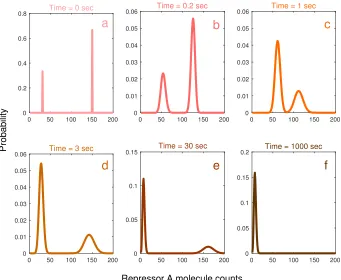
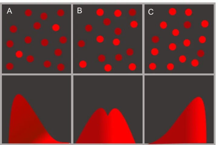
Figure 2.1: Schematic representation of the fluorescence of anE. colicell pop-ulation that carries the genetic toggle switch. The stochastic gene expression of red fluorescent reporter proteins inE. colicells that carry the genetic toggle switch from [GCC00] creates a distribution of phenotypes. The reporter protein fluoresces red such as mCherry [Sha+04]. In panels A, the cell phenotypes form a unimodal distribution that peaks at a low (dark red) fluorescence level. A few cells have high (bright red) fluorescence levels and they represent the tail of the distribution of phenotypes. In panel B, the cell phenotypes form a bimodal distribution with peaks at both a low (dark red) and a high (bright red) fluorescence level. In panel C, the cell phenotypes form a unimodal distribution that peaks at a high (bright red) fluorescence level. Data measurements and discussion corresponding to this schematic are available in [GCC00;Por+07].

The shortage of analytical solutions to the CME model poses a challenge to the engineering design cycle in Chapter 1 for the field of synthetic biology. In this chapter, we aim to mitigate the lack of analytical solutions to the CME through our design framework, which does not make use of analytic solutions. We first design the stationary behavior of a transcriptional network for which we have computed an analytical solution to the CME model [GD12;Men+17]. Subsequently, we propose a framework for the design of stochastic behaviors of biochemical reaction networks, irrespective of the analytical solutions to their CME models.

(31)

MA09] and power systems that use renewable energy sources such as wind or solar power [GA14]. Nonetheless, stochasticity can sometimes confer increased flexi-bility to uncertainty, as demonstrated by bet hedging strategies in bacterial persis-tence [VSK08;Bal+04] and in delayed seed germination in plants [Coh67]. There-fore, designing for stochastic behaviors is beneficial to some systems. Stochastic design specifications are encountered in applications where stochasticity is essential and stochastic models are ubiquitous, such as turbulent flow models for aerodynam-ics and for oceanography [GM13]. There, mathematical tools for stochastic PDEs inform the stochastic design constraints for turbulent flow models [Pop02].

The design features we propose for biological systems are inspired by unanswered questions in the design of genetic regulatory circuits. Our insight comes from the problem of designing the stochastic behavior of the genetic toggle switch in [GCC00]. Gene expression levels in cells of an E. coli population carrying the toggle switch form a distribution of phenotypes due to the heterogeneity of the cell population [Por+07], as illustrated in Figure2.1. This distribution of cellular phenotypes follows either unimodal, bimodal, or trimodal stochastic transient and stationary behaviors [KRS15; Sch+10]. The phenotypic heterogeneity of the cell population is not typically designed for or specified. We can help control this hetero-geneity by specifying the modality of the transient distributions: uni-/multi-modal, the protein expression levels, and the switching time. We mathematically formulate these design specifications similarly to [MG09] and we discuss how they result in remarkably different behaviors in a cell population.

Our design framework captures both stationary and transient distributional behaviors of biochemical networks such as uni-/multi-modality, the locations of the modes, and the rate of convergence to stationarity. These design features could not be captured by a deterministic framework; even the first moment, the single mode of a unimodal distribution, might be altered by stochastic effects [PBE00].

(32)

to combine orthogonal basis polynomials in the space of projection so that they ex-pressed the design features of uni-/multi-modality of distributions. This formulation would create overly elaborate problems that lose track of biological implementa-tion. To avoid these issues, we simply consider the Taylor approximation to the exponential operator and we compute bounds on the error of this approximation. If we use a first order Taylor approximation to the exponential operator, the de-sign problem reduces to solving a linear program and a semi-definite optimization program [XB04; BV04]. There exist very efficient, scalable convex optimization tools, such as CVX [GBY08;GB08], that solve these programs. If the error of the first order Taylor approximation is large, we suggest using polynomial optimization methods as an alternative. Solving the design problem depends on the number of design features and the number of molecule counts of each biochemical species, particularly in the polynomially constrained case. Ultimately, we show that we can find accurate solutions for biochemical reaction networks with several species by using a first order Taylor approximation.

This chapter is organized as follows: In Section 2.2, we solve the design problem for a transcriptional network with a known analytical solution to the CME model. In Section 2.3, we set up the design problem and evaluate the error in the ap-proximation of the exponential operator. In Section 2.4, we implement and solve design problems for classic examples of biochemical reaction networks: protein production-degradation, the Schlögl model, and the genetic toggle switch. Sec-tion 2.5 contains discussion of the applicability and limitations of our stochastic design framework, as well as an outline for future work.

2.2 The Design Of Stationary Stochastic Behaviors Of Biochemical Reaction

Networks Using Analytical Solutions

In this section, we illustrate how the design of the stationary behavior of the tran-scriptional network in [GD12] is simplified by the availability of an analytical solution to its CME model. The analytical solution was first derived in [GD12] by applying the deficiency zero theorem from [ACK10] and then in [Men+17] by adapting the graph gluing technique proposed by Mélykútiet al.[MHK14;MP15]. No analytical transient solutions to the CME model of this transcriptional circuit are available, although an approximation was derived in [GD12] using singular perturbation theory [DM15].

(33)

de-sign the equilibrium behavior of the transcriptional circuit simply by tuning the reaction rate parameters. This corresponds to altering the transcription factor’s production or degradation rates, or its binding and unbinding rates to the down-stream DNA. Tuning these rates can be implemented by choosing a transcription factor with the desired strength of binding and unbinding to DNA, by making more RNA polymerases or coactivators available to increase the transcription rate, by adding ubiquitin [DRH00], by tagging for phosphorylation [Gri+98] to increase the transcription factor’s degradation rate, or even by changing the response element. We first describe the two-component transcriptional system in Figure2.2 [GD12]. The two transcriptional components are connected to each other through the action of the transcription factor Z. In the upstream component, Z is both produced and degraded. In the downstream component, transcription factor Z binds to DNA binding sitesP and forms the complexC. The total amount of DNA, which is the sum of free binding sites P and of the complexC, is assumed to be conserved. We model the two-component transcriptional system stocastically using the chemical reactions in equation (2.1):

Z−−−)−−−k* δ

∅,

Z+P−−−₎k₋₋₋on*

koff

C.

(2.1)

We let c be the number of molecules of the complex C and z be the number of molecules of transcription factor Z.

(34)

Z

k

ẟ

Upstream Component

P

C

k

_off

k

_on Downstream

Component

Figure 2.2: A biological system of two interconnected transcriptional compo-nents [GD12]. In the upstream component, proteinZ is transcribed from the DNA at rate k and degraded at rate δ. In the downstream component, protein Z acts as an activator that binds the DNA binding sites P and forms a complex C with it. Transcription factorZ and DNA sitesPbind together with ratekonand unbind with

ratekoff. The total DNA is conserved, so the amount of DNA bound to transcription

factorCand the amount of free DNA binding sitesPis assumed to be constant.

of transcription factors in equation (2.2):

P(c,z)=

1+ κκon

δκoff

−N

N c

κκon

δκoff

c

e−κ/δ(κ/δ)

z

z! (2.2)

forc ∈ {0, . . . ,N}andz,N ∈_Z_≥0.

At stationarity, the upstream and downstream transcriptional systems are indepen-dent since the product of the stationary distributions of transcription factor Z and complexC equals their joint stationary distribution. This indicates that the system is not subjected to retroactivity at stationarity, meaning that the interconnection between the upstream and downstream modules does not slow down the dynamics of the upstream module [DM15; DDQ16]. Consequently, the expected value of their joint stationary distribution can be determined from the expected values of the transcription factorZ and of the complexC.

(35)

global maximum simplifies the subsequent design of its location, as illustrated in Figure2.3. We present the proof of Theorem2.1in AppendixA.

Theorem 2.1. Consider the system of two interconnected transcriptional compo-nents that are modeled by reactions as given in equation (2.2), where κ >0, δ >0,

κon > 0, and κoff > 0are the corresponding reaction rate constants. LetP, Z, and

Cbe the numbers of promoters, transcription factors, and complexes, respectively. Letα = κκon

δκoff, β=

κ

δ, andγ = Nαα+1−1, whereN is a constant given by N = P+Cdue

to the conservation of DNA. In (i)–(iii), we set up and solve three design problems using the marginal stationary distributions ofZandC. Here,αandβare the design variables.

(i) Since the marginal stationary distribution of Z is a Poisson distribution, its mean and variance are equal. The design problem of fixing the mean of Z at an objective value µz > 0is feasible, and the solution is β = µz, with N and

the reaction rate constants being arbitrary otherwise.

(ii) The design problem of setting the mean ofCat an objective valueµc ∈ (0,N)is

feasible, and the solution isα= µc

N−µ_c, withN and the reaction rate constants

being arbitrary otherwise.

(iii) The design problem of choosing the variance ofCto be an objective valueσ_c2>

0is feasible if and only ifσ_c2≤ N

4, and the solutions areα=

N−2σc2±

√

N2₋_4N_σ2 c

2σc2 ,

withNand the reaction rate constants being arbitrary otherwise.

(36)

Corollary 2.3. Under the constraints N > 1, β > 1, 0 < γ < N −1, and β, γ _< Z, designing the location of the unique global maximum of the two-component transcriptional system modeled by the reactions in equation (2.2) is equivalent to findingN, β, andγsuch that(bγc+1,bβc)is the objective location.

When the global maximum of the two-component transcriptional system exists and is unique, there are infinitely many parameter values that can lead to the objective location of the global maximum. Since anyα, β,γ, andNthat satisfy the conditions in Corollary 2.3 lead to the desired global maximum design, this implies relative insensitivity with respect to experimental implementation.

Figure 2.3: Designing the global maximum of the joint stationary distribution of the complex species and the transcription factor species using its analytical form. We consider the transcriptional circuit in [GD12] and we state the analytical form of the stationary distribution of the complex and the transcription factor species in equation (2.2). We then apply Proposition 2.2 and Corollary2.3 to design the location of its global maximum. The parameter values we use are as follows:

N = 10 molecules,α= 2, β= 5.5,γ = 6.33. The joint probability distribution has a unique global maximum at 7 molecules of the complexC and 5 molecules of the transcription factorZ.

(37)

factor with promoters, and the total amount of DNA, as illustrated in the example in Figure2.3. In Section2.3, we consider designing similar features for distributions of reactant species in biochemical reaction networks when analytical solution to their CME models are unknown.

2.3 The Design Of Transient And Steady State Stochastic Behaviors Of

Bio-chemical Reaction Networks

The design problem formulation

Our formulation of a stochastic design framework for biochemical reaction networks is a two-part contribution. We mathematically describe the desired transient and stationary behavior with design features and we find a solution for the design problem under these constraints. We then illustrate this stochastic design framework on several examples of biochemical reaction networks.

The design features

The design features we choose to constrain the stationary and transient probability distributions of biochemical species are as follows:

(i) uni- or multi-modality (ii) the locations of the modes

(iii) the rate of convergence to stationarity

Our inclusion of design feature (i) is motivated by experimental evidence that demonstrates the presence of multi-modality in the genetic switching of the λ phage in the lactose operon [CLL10], in stochastic gene expression [SS08], and in cellular signal transduction pathways in mammalian cells [TB06]. The Gardner et al. genetic toggle switch [GCC00] is the first synthetic gene regulatory circuit to display multi-modality. An illustration of the genetic toggle switch’s stochastic behavior is presented in Figure2.1. Further discussion of the genetic toggle switch is available in Gardneret al. and Portleet al.[GCC00;Por+07]

(38)

The design problem as an optimization program

We now consider the mathematical formulation of the design problem that incorpo-rates the design features (i) - (iii). We assume a biochemical reaction network model with unknown reaction rate parameters subjected to these design constraints. We use the same notation for the biochemical reaction network and for the chemical master equation as in Chapter1, but we replace the transition matrix H(c)corresponding to the continuous CME with the matrix D(c)that corresponds to the approximate discrete time dynamics:

D(c)= dtH(c)+_IM×M (2.3)

In the design problem formulation we want to find the reaction rate vector c =

(c1, . . . ,cM)of the biochemical reaction network such that the transient (or

station-ary) probability distribution vectorp(x,t)is constrained according to our choice of design features at time points t ∈T = {t1, . . . ,tk}, where k ≥ 1 is the number of

time points. Additionally, the dynamics of the probability distribution vectorp(x,t) are constrained by the CME. Lastly, we want to control the convergence rate of the transients to stationarity. These constraints and variables result in the following optimization program:

Findc= (c1, . . . ,cM)such that

f0p0 ≤ µ0, f p∗ ≤ µf, (2.4)

fieH(c)tip0 ≤ µi, (2.5)

(D(c) −p∗1M)T(D(c) −p∗1M) ≤ µ2IM×M, (2.6)

D(c)p∗ = p∗, (2.7)

H(c)= ΣM_j₌₁cjHj, (2.8)

p0 ∈ X0,p∗ ∈ Xf,pti ∈ Xi, (2.9)

X0,Xi,Xf ⊆ P,∀1 ≤i ≤ k, (2.10)

where p0 and p∗ are the initial and stationary distributions, respectively; f0, fi, f

are pre-selected projection operators that result in uni- or multi-modality of distri-butions; X0,Xi,Xf are pre-selected subsets of P; µ, µi, µf are the tightness of the

bounds, for all 1≤ i ≤ k.

(39)

stationary distributions are constrained by projection operators f0, fi, f, respectively

for 1 ≤i ≤ k. An example of operator that imposes unimodality and the locationm

of the mode is the functiong:_R≥0 →R≥0,g(x)= (x−m)2[MG09]. In Section2.4,

we give more examples of projection operator choices.

As shown in [XB04], the inequality in equation (2.6) uses the bound µto tune the largest singular value of matrix H(c). Thus, µcontrols the rate of convergence to the stationary distribution. The inequality reduces to a semi-definite constraint by using the Schur complement formulation in [BV04].

The equality in equation (2.7) specifies thatp∗is the stationary probability distribu-tion vector of the Markov process, as explained in [XB04].

Remark 2. We clarify that design features (i) and (ii) apply to the marginal prob-ability distributions of biochemical reactants in networks with more than just one species, N > 1. In order to marginalize the probability distributions, we multiply the operators f, f0and fi,1 ≤i ≤ k, by the appropriate marginalization matrices of

sizesM ×MN−1.

Remark 3. In practice, we choose to implement the design problem to minimize the linear objective function given by the sum of the boundsµ0+µ1+. . .+µk+µf+µ

with respect to the rate reaction rate vectorc=(c1, . . . ,cM)under the constraints in

equations (2.4-2.10). When the bounds µ0, µ1, . . . , µk, µf, µ are pre-specified, the

design problem reduces to finding a reaction rate vector c that satisfies equations (2.4- 2.10), if c exists. Thus, the optimization program simplifies to a feasibility problem.

Finding a solution to the design problem

Our main challenge in finding a solution to the design problem is the exponential operator present in equation (2.5). Our best approach has been to consider the Taylor approximation to the exponential operator and calculate the error of this approximation. Using the Taylor approximation of order l ≥ 1 of the exponential operator, the inequality in equation (2.5) is replaced by

fi l

Õ

v=0

1

v!(H(c)ti) v_p

0 ≤ µi,∀1 ≤i ≤ k. (2.11)

(40)

(2.7) and (2.11). The problem is polynomial of degree l +1 in variables c, p0,

and p∗ [BV04]. In Section 2.4, we find it useful to assume knowledge of p0 and

p∗, acquired either through experimental data or by computer simulations. This reduces the degree of the polynomial problem to l, eliminates equation (2.4), and makes equation (2.7) linear. The design problem in equations (2.4-2.11) is now a polynomial optimization program of degreel. In Section2.4, we assumel = 1, so the equality in equation (2.11) is also linear. We then use CVX [GBY08;GB08] to solve the resulting optimization problems in Section2.4.

Remark 4. There is a clear trade-off between choosing a larger truncation orderl

with the effect of decreasing the approximation error and keeping the degree of the polynomial inequalities in the design problem low.

2.4 Implementation of the Stochastic Design Framework

The protein production-degradation reaction network

We implement our design problem formulation to the gene regulatory network of protein production and degradation in [DM15]. Here, protein production and degra-dation are modeled stochastically as a birth-death Markov process. The chemical reaction network has only two reactions:

A−−−₎₋₋₋c1*

c2

∅. (2.12)

The reactions in equation (2.12) model the production and degradation of protein species A. The rates of the two reactions arec1andc2. The birth occurs according

to a Poison process with probability c1 per unit time and the death occurs with

probability per unit time proportional toc2A(t). The analytic solution to its chemical

master equation isp(t)= c2 c1(1−e

−c₁t₎_[GS01].

We choose the transient distribution to be unimodal with a single mode at 100 proteins using the operator f(x) = (x−100)2and find the chemical reactions that satisfy this constraint. We assume that the stationary distribution is pre-determined by a Gaussian distribution with the same mean. The initial probability distribution is a Dirac delta function of height 1. Matrices H1 and H2 in equation (1.19) of

Chapter1are the same as in [MG09].

Our stochastic design framework finds optimal reaction rates c1 = 3.9894 and

c2 = 0.0397. The number of states in the FSP truncation is S = 201 and the

(41)

[image:41.612.128.474.84.366.2]

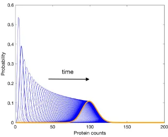
Figure 2.4: Solution to the design problem for a protein production-degradation reaction network. Time evolution of the unimodal transient distributions in the birth-death process in chemical reactions2.12. The transient distribution after 100 seconds is displayed in orange and it has a single mode at 100 protein counts. The previous transient distributions are displayed in blue and they are indeed uni-modal. The black arrow indicates the transients’ progression towards stationarity as a function of time.

is O(10−9). The results are illustrated in Figure2.4. For a comparison of the last transient in Figure2.4and the stationary distribution, see FigureA.1in AppendixA. Remark 5. The solution to the optimization problem is not unique. The reaction rates c1 and c2can take other values and they can certainly be adjusted by tuning

the bounds µ0, µ1, . . . , µk, µf in equations (2.4-2.10).

The Schlögl chemical reaction network

(42)

reactions in the Schlögl network are as follows:

A+2X−−−₎a₋₋₋1*

a2 3 X,

B−−−₎a₋₋₋3*

a4 X.

(2.13)

The concentrations of chemical speciesAandBare buffered and the four propensity functions are as follows:

a1(X)= k1A

1

2X(X−1),

a2(X)= k2

1

6X(X−1)(X −2),

a3(X)= k3B,

a4(X)= k4X,

(2.14)

wherek1,k2,k3,andk4are the reaction rates.

We return to our previous notation by setting c1 = k1A, c2 = k2, c3 = k3B, and

c4 = k4. The analysis of the deterministic model of the reaction network informs

us that there exists a bifurcation with two equilibrium values of s1 = 84.79 and

s2 = 569.9. We construct our projection operators to be centered around these

values.

Using operator funimodal(x) = (x − s1)2, we impose unimodality on the transient

distributions and we find optimal rate reaction values c1 = 1.0710×10−5, c2 =

21.9939× 10−15, c3 = 0.3668, and c4 = 0.0049. We expect the reaction rate

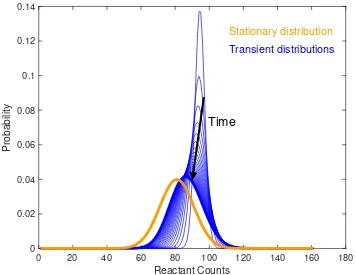
values to span several orders of magnitude [Gun+05]. The convergence rate in the application of our stochastic design framework is µ = 0.001. This result is illustrated in Figure2.5.

Alternatively, we can also impose a bimodal transient constraint as in [MG09] using projection operator

fbimodal(x)=

(

min((x−s1)2,14920) ifx ≥ 328

min((x−s2)2,14920) otherwise.

(2.15)

and, simultaneously, a unimodal stationary constraint f∗(x) = (x−s1)2. A plot of

the bimodal projection operator is available in FigureA.2in AppendixA.

The results of stochastic design framework are illustrated in Figure 2.6. We start from an initial distributionp0consisting of two Dirac delta functions with different

(43)

0 20 40 60 80 100 120 140 160 180 Reactant Counts

0 0.02 0.04 0.06 0.08 0.1 0.12 0.14

Probability

Time

Stationary distribution

[image:43.612.126.482.81.356.2]

Transient distributions

Figure 2.5: Solution to the design problem for the Schlögl reaction network with unimodal transient constraints. We plot the time evolution of the unimodal transients and compare it to the the stationary distribution. We find optimal rate reaction values c1 = 1.0710× 10−5, c2 = 21.9939 × 10−15, c3 = 0.3668, and

c4= 0.0049 with a convergence rate to stationarity ofµ= 0.001. Not all transients

are displayed.

distribution p∗. It is possible to find a solution to the problem almost irrespective of the placement and the heights of the Dirac delta functions. We demonstrate this in Figure 2.7 with a different unimodal stationary distribution choice of f∗(x) = (x − s2)2. It is also possible to define an initial distribution p0 with Gaussian

distributions replacing the Dirac delta functions. We can also replace the piece-wise function with a sum of Gaussian distributions centered ats1ands2. In all these

cases, we are able to obtain solutions to the stochastic design problem.

(44)

0 200 400 600 800 0

0.2 0.4 0.6

0.8 Time = 1 sec

0 200 400 600 800 0 0.01 0.02 0.03 0.04 0.05

0.06 Time = 500 sec

0 200 400 600 800 0 0.005 0.01 0.015 0.02 0.025

0.03 Time = 2000 sec

0 200 400 600 800 0 0.005 0.01 0.015 0.02 0.025

0.03 Time = 5000 sec

0 200 400 600 800 0 0.005 0.01 0.015 0.02 0.025

0.03 Time = 8000 sec

0 200 400 600 800

Reactant counts 0 0.01 0.02 0.03 0.04

Probability Time = 10000 sec

b c

d _e _f

[image:44.612.132.471.83.362.2]

a

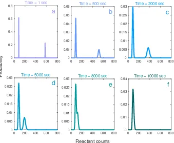
Figure 2.6: Solution to the design problem for the Schlögl reaction network with bimodal transient constraints. We plot the time evolution of the distributions. In part a, the initial distributions is pictured. We move through the bimodal transients in parts b-e. Part f has the stationary distribution. Not all transients are displayed.

the desired stationary distribution p∗, but it ultimately decays to a stationary dis-tribution corresponding to the eigenvector with the largest eigenvalue. We choose not to implement equation (2.7) without the relaxation because the problem can be infeasible.

The genetic toggle switch

(45)

0 200 400 600 800 0

0.2 0.4 0.6

0.8 Time = 1 sec

0 200 400 600 800 0

0.01 0.02 0.03

0.04 Time = 10000 sec

0 200 400 600 800 0

0.005 0.01 0.015

0.02 Time = 50000 sec

0 200 400 600 800 0

0.005 0.01

0.015 Time = 100000 sec

0 200 400 600 800 0

0.002 0.004 0.006 0.008

0.01 Time = 200000 sec

0 200 400 600 800

Reactant Counts

0 0.002 0.004 0.006 0.008 0.01

Probability Time = 1000000 sec

a _b _c

d _e _f

Figure 2.7: Solution to the design problem for the Schlögl reaction network with bimodal transient constraints We plot the time evolution of the distributions. In part a, the initial distributions is pictured. We move through the bimodal transients in parts b-e. Part f has the stationary distribution. Not all transients are displayed.

Inducer I

Reporter

[image:45.612.122.471.94.379.2]

Repressor B Promoter A Promoter B Repressor A