A fast multiple mode intermediate level circuit model for the prediction of shielding effectiveness of a rectangular box containing a rectangular aperture

(1)

This is a repository copy of A fast multiple mode intermediate level circuit model for the prediction of shielding effectiveness of a rectangular box containing a rectangular aperture. White Rose Research Online URL for this paper:

http://eprints.whiterose.ac.uk/132800/

Article:

Konefal, T, Dawson, J F orcid.org/0000-0003-4537-9977, Marvin, A C

orcid.org/0000-0003-2590-5335 et al. (2 more authors) (2005) A fast multiple mode

intermediate level circuit model for the prediction of shielding effectiveness of a rectangular box containing a rectangular aperture. IEEE Transactions on Electromagnetic

Compatibility. pp. 678-691. ISSN 0018-9375 https://doi.org/10.1109/TEMC.2005.853715

Reuse

["licenses_typename_other" not defined]

Takedown

If you consider content in White Rose Research Online to be in breach of UK law, please notify us by

(2)

A fast multiple mode intermediate level circuit model

for the prediction of shielding effectiveness of a

rectangular box containing a rectangular aperture

T. Konefal, J.F. Dawson, A.C. Marvin, M. P. Robinson and S.J. Porter

Abstract

This paper presents an intermediate level circuit model (ILCM) for the prediction of the shielding effectiveness (SE) of a rectangular box containing a rectangular aperture, irradiated by a plane wave. The ILCM takes into account multiple waveguide modes, and is thus suitable for use at high frequencies and/or relatively large boxes. Inter-mode coupling and reradiation from the aperture are taken into account. The aperture may be positioned anywhere in the front face of the box, and the SE at any point within the box may be found. The model is presented in such a way that existing ILCM techniques for modelling elements such as monopoles, dipoles, loops or transmission lines may be seamlessly incorporated into the circuit model. Solution times using the ILCM technique are hundreds of times less than those required by traditional numerical methods such as FDTD, TLM or MoM, even when using a relatively slow interpreted language such as MATLAB. Accuracy however is not significantly compromised. Comparing the circuit model with TLM over nine data sets from 4MHz to 3GHz resulted in an rms difference of 7.70dB and mean absolute difference of 5.55dB in the predicted SE values.

Keywords:

Circuit model, multiple modes, shielding effectiveness, aperture in box.

1 Introduction

A frequently occurring problem in electromagnetic compatibility (EMC) is the determination of the electromagnetic fields inside an enclosure containing apertures. In many cases the enclosure and apertures are rectangular, and this has led to a number of attempts at solving the problem of a rectangular box with a rectangular aperture, irradiated by a plane wave. For example, in [1-4] the electric field integral equation (EFIE) is used to solve the problem using the Method of Moments (MoM). Although the treatment of the aperture is efficient, this self-consistent method is still computationally intensive. Indeed, using a variety of standard numerical techniques such as Finite Difference Time Domain (FDTD), Transmission Line Matrix (TLM) or Method of Moments (MoM), the problem is readily tackled e.g. [5-7]. Unfortunately there can often be some differences in the solutions in critical regions using these techniques, depending on the slight differences in spatial, time or frequency resolution chosen for the computer simulations, and indeed on the precise simulation method chosen. A purely analytic approach is described in [6], though even in this case we are forced to truncate an infinite series at some suitable point, and the method effectively becomes a MoM solution. However, the main problem with such techniques is that they all require significant computer resources such as RAM and/or hard disk space, and can take several hours, days or even weeks to reach a solution. This is true despite the

(3)

significant and continuing improvement that has been made in commonly available computing resources in recent years. (Clock speeds of 2-3GHz are typical of computing equipment at the time of writing).

The slowness of solution using these methods has prompted a number of investigators to try and find a more rapid solution to the problem, using various approximations. One of the first successful techniques was that due to Robinson et al. [8], who used an equivalent circuit technique to find a sufficiently accurate frequency domain solution to the problem in just a few lines of computer code, taking only a small fraction of a second. The original solution of [8] is limited in its scope in a number of ways. The incident plane wave can only have one polarization and direction of travel, though fortunately this is often the worst case as far as shielding effectiveness (SE) is concerned. In addition, the rectangular slot must be centrally placed in both height and width in the rectangular front face of the box. However, the most severe limitation of the model in [8] is that the model considers only the excitation of the TE10

mode of the box. This limits the accuracy of the solution to low frequencies and/or relatively small boxes, where the TE10 mode is dominant. We note here that the model has no difficulty

with dealing with an exponentially decaying (evanescent) mode, below the TE10 cut off

frequency. However, at frequencies where higher order modes can propagate, the model becomes inaccurate. For reasonably large boxes, of the order 0.1m3 , the scope of the model in [8] is thus limited to a few hundred MHz.

The problem of oblique incidence of irradiation has been addressed in [9], whilst still retaining only the TE10 mode. The aperture is treated as a two-wire transmission line with no radiation

losses. The treatment is extended in [10] to take into account multiple modes, though only frequencies below 1GHz are considered. In fact, only one of the results presented in [10] involves a higher order propagating mode below 1GHz, and in this particular case there is a feature in the predicted SE just below 700MHz, corresponding to the TE201 resonance [11],

which is not observed in experiment. (In this particular case the TE20 mode begins to propagate

above 621MHz). Another attempt at a multimode treatment of the aperture in a box problem has been made in [12], though curiously only TEm0 and TM1n modes are considered, making the

theory totally unsuitable for prediction of SE for off-centre positions in the box. Indeed, no direct comparisons with numerical results on the same graph are given, and an unknown empirical loss factor is introduced into the model. In all of the models [8-10] and [12], only apertures centrally placed in height and width in the front face of the box are considered.

(4)

of the radiation resistance. The resultant aperture field is used to give a first estimate of the modal excitation of the box, under the temporary assumption that the presence of the box does not affect the aperture field. However, unlike the model of [10], the aperture field is then allowed to be altered by energy entering and exiting the box, taking into account inter-mode coupling and energy reradiation into free space. The model thus accounts for all the physical processes present.

The ILCM model can cope with rectangular apertures positioned anywhere in the front face of the box, unlike the models of [8-10] and [12]. However, it is most accurate for ‘slot’ type apertures where the height of the slot is significantly less than its length (say less than 12%). Any direction of incidence and polarisation of the incoming plane wave may be dealt with in the theory, though we have only been concerned with yˆ polarized waves travelling in the +zˆ

direction. In addition, the model can readily be used at high frequencies (we have set an upper limit of 3GHz for convenience) without deterioration in accuracy, providing an appropriate number of modes are taken into account.

The circuit model is rapid, taking typically less than 30 seconds to process 750 frequency data points using a relatively slow interpreted language such as MATLAB. This contrasts with a typical run time of four and a half hours for the numerical technique of Transmission Line Matrix (TLM) modelling. Despite its simplicity, the ILCM model is remarkably accurate, showing an overall rms difference in SE values of 7.70dB compared with TLM, and a mean absolute difference of 5.55dB. Visual examination of the curves in Section 6 supports the validity of the circuit model, with the vast majority of the many features in the TLM simulations reproduced by the circuit theory.

Sections 2 and 3 describe the problem at hand, and give an initial solution for the field in the aperture, in the absence of the rest of the box. Sections 4 and 5 explain how this aperture field is modified by the presence of the box, and develop an equivalent circuit to model the inter-mode coupling and reradiation into free space. The circuit model results are compared with the numerical method of TLM in Section 6, with some conclusions being drawn in Section 7.

2 Plane wave excitation of a rectangular box containing a

rectangular slot

2.1 Experimental Configuration

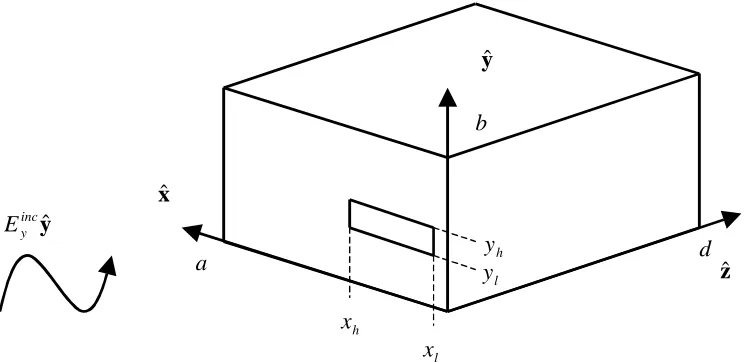
Figure 1 shows the experimental configuration that it is desired to model using circuit theory. A rectangular box of dimensions a(x)×b(y) ×d(z) contains a rectangular aperture in its front face

(z=0) extending from x=x_l to x=x_h and y= y_l to y= y_h. The box is irradiated by an incident plane wave Eyinc, polarized in the yˆ direction and travelling in the +zˆ direction. The

(5)

much less than a wavelength of free space radiation at the frequency of irradiation of Eincy .

Under these conditions, and particularly if (y_h −y_l)<<(x_h −x_l), the slot can be approximated to a section of coplanar strip transmission line that has been short-circuited at x and l x . When h

the aperture or slot is centrally placed in the front panel, it is possible to assign a quasi-static characteristic impedance to this transmission line [19]. However, for the purposes of this paper we need the slot transmission line to have the same characteristic impedance as the quasi-TEM wave it supports. This is necessary to be consistent with the general theory of analogous transmission lines described in [14][20], where the analogous transmission line representing a waveguide mode is assigned the same characteristic impedance as the transverse ratio of E and H fields that the mode supports. The ‘analogous’ transmission line (rather than the literal transmission line) representing the slot is therefore assigned a characteristic impedance of

Ω =377

FS

Z , the impedance of free space. This assignment is not only found to improve the quality of the results (see Section 6) but also negates the need to work out the characteristic impedance when the slot is not placed at the central height of the front panel.

yˆ

zˆ

a

b

d

yˆ

inc y E

xˆ

l x h

x

l y

[image:5.595.116.488.345.526.2]

h y

Figure 1. Slot in box irradiated by incident field Eincy , showing box

dimensions and slot dimensions.

2.2 Plane wave excitation of a two-wire transmission line

The analysis in this section is similar to that given in [9]. Consider a two-wire transmission line of length xh −xl aligned in the xˆ direction and with a vertical separation g= yh −yl in the yˆ

direction. The line is situated in the plane z=0 and is illuminated by a plane wave travelling in the direction bˆ . The incident electric and magnetic fields are related by

inc inc

FS

Z H =bˆ×E (1)

(6)

) exp( ) , , ( r

E = E E Ezinc −j ⋅

inc y inc x inc (2) ) exp( ) , , ( r

H = H H Hzinc −j ⋅

inc y inc x inc (3) b

bˆ ˆ

) , , ( c z y x ω β β

β = =

= (4)

The transmission line equations of the system, including the forcing terms of the external applied fields, can be solved as in [9] to give the voltage V(x) on the transmission line i.e.

) exp(

exp exp

)

( x H j x

c j B x c j A x

V ω ω + − β_x

    − +      +

= (5)

where ) ( 2 2 2 0 2 2 c c T H E c H x x y inc z x inc y ω β β ω β ωµ ω ≠ −       ₊

= (6)

      = − ≠         − − = 0 for 0 for ) exp( y l h y y y y y y y y j y j T h l β β β β (7)

and A and B are determined by the boundary conditions of short circuits terminating the line in the planes x=x_l and x=x_h i.e. V(xl)=V(xh)=0. Thus

      − − − −       − + − + =       − ) exp( ) exp( ) / exp( ) / exp( ) / exp( ) / exp( 1 l x h x l l h h x j H x j H c x j c x j c x j c x j B A β β ω ω ω ω (8)

Equations 5-8 define the solution to the voltage V(x) on the two-wire transmission line.

The solution of Equation 5 can be used to find the field Eywire between the two wires of the

transmission line i.e.

(

j x

)

g H x c j g B x c j g A g x V y y x V E x l h wire y β ω

ω ₋ ₋

     − −      + − = − = − −

= ( ) ( ) exp exp exp (9)

We now make the assumption that the field Eyaperture(x) in the slot of Figure 1, in the absence of

(7)

l y y≤

≤

0 and yh ≤ y≤b. Providing b is small compared to a wavelength, this should be a

good assumption, since when viewed in the plane z =0 the two-wire transmission line appears as a short dipole whose length has been extended by the factor (b/g), with a corresponding increase in antenna factor of (b/g). This should also serve as a reasonable first approximation for the increase in field when b is comparable to a wavelength. The aperture field in Figure 1, in the absence of the rest of the box in the region z>0, is thus estimated as

(

)

_

  



 ₊ ₋

   

 − +

   

 + −

= x H j x

c j B

x c j A

g b x

Eaperture _x

y β

ω ω

exp exp

exp )

( ₂ (10)

Equation 10 does not take into account the energy that enters and exits the box, nor does it take into account (in free space) any reradiated energy. The latter aspect is dealt with in the next section, which uses the Numerical Electromagnetics Code (NEC) [17] in conjunction with the Babinet principle [18] to assign a radiation resistance to the original two-wire transmission line problem. This modifies the solution for Eyaperture(x) given by Equation 10 and significantly reduces the Q factor of the undesirable strong resonance that would otherwise occur when the slot length (x_h −x_l) corresponds to a half wavelength of radiation. Note that Equation 10 permits arbitrary angles of incidence for a plane wave, though for the sake of brevity we have been concerned in this paper only with plane waves for which βx =0,βy =0.

3 Modification of the aperture field in free space by inclusion of

radiation resistance

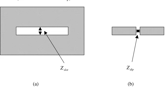
3.1 Use of NEC to find radiation resistance

slot

Z Zdip

(Metal extends to infinity)

[image:7.595.112.452.529.706.2]

(a) (b)

(8)

Figure 2 shows two complementary structures where metal is replaced by free space and vice versa. From Babinet’s principle [18] the impedances of the two structures at the points shown are related by

4

2

FS dip slot

Z Z

Z = (11)

where ZFS is the impedance of free space (ZFS =377Ω). In order to find the impedance Zslot

therefore, we simulate the impedance of the planar dipole of Figure 2(b) using the Numerical Electromagnetics Code (NEC) [17]. This is very rapid, and typically will take less than a second for 750 data points. In practice, if the width w and the length l of the planar strip are

l h y y

w= − , l =x_h −x_l, a reasonable approximation to the impedance Z_dip can be found by simulating the impedance at the centre of a wire dipole of length l and radius r where πr=w. From Equation 11, the corresponding impedance Zslot of Figure 2(a) may be found. Note that

the NEC simulation will generate a value of Z_dip which has a real component, representing the radiation loss mechanism into free space. Similarly, Zslot will have a real component, also

representing the radiation loss mechanism into free space. It is this resistance which is used to modify the solutions for V(x) and Eaperturey (x) given by Equations 5 and 10 respectively, in the absence of reradiation from the slot. Note that we do not in fact have an infinite sheet of metal surrounding our slot in Figure 2, so that this treatment is approximate.

3.2 Calculation of parallel radiation resistance of slot

From simulation using NEC, the impedance of the dipole of Figure 2(b) is given by

d d dip R jX

Z = + (12)

From the transmission line point of view, Z_slot in Figure 2 can be considered as two short circuited sections of transmission line connected in parallel (a pure reactance) in parallel with a radiation resistance R . Manipulating Equations 11 and 12 yields the parallel radiation _p

resistance R in terms of the dipole resistance _p R simulated in NEC as d

d FS p

R Z R

4

2

= (13)

Thus from NEC simulation of the dipole in Figure 2(b), it is possible via Equations 12 and 13 to find the equivalent radiation resistance R strapped across the centre of the slot in Figure 2(a). p

(9)

[image:9.595.103.511.274.417.2]

3.3 Solution for aperture field

Eyaperture(x)

in the presence of

Rp

Figure 3 illustrates a two-wire transmission line, irradiated externally by a plane wave travelling in the bˆ direction. In the absence of any reradiation from the line, the solution for the electric field between the wires is given by the aperture field Eyaperture(x) in Equation 10 with

g y y

b= _h − _l = .

inc

E

inc

H

b

p R

RHS I LHS

I

rad I

l x h

x l

y h y

Figure 3. Transmission line with radiation resistance R , irradiated by plane wave. p

We wish to calculate the field on the line in the presence of R , the radiation resistance that p

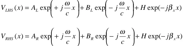
enables energy to be lost from the line by the process of reradiation. Following the method in Section 2.2, we can write the solution for the voltages on the left hand side (LHS) and the right hand side (RHS) of R as p

) exp(

exp exp

)

( x H j x

c j B

x c j A

x

VLHS L L βx

ω

ω ₊ ₋

   

 − +

   

 +

= (14)

) exp(

exp exp

)

( x H j x

c j B

x c j A

x

VRHS R R βx

ω

ω ₊ ₋

   

 − +

   

 +

= (15)

with corresponding solutions for the LHS and RHS currents given by

) exp(

exp exp

)

( 0

0 x Z H j x

c j B

x c j A

x I

Z _s _LHS _L ω _L ω + _s ′ − β_x

  

 − +

   

 + −

= (16)

) exp(

exp exp

)

( ₀

0 x Z H j x

c j B

x c j A

x I

Z _s _RHS _R ω _R ω + _s ′ − β_x

  

 − +

   

 + −

[image:9.595.70.364.536.611.2]

(10)

Here Z₀_s is the characteristic impedance of the transmission line (which we will eventually take to be ZFS =377Ω) and

[

]

) ( 2 2 2 0 2 c c T C H E H x x y l inc z inc y x ω β β ω µ ω ωβ ≠ − + =

′ (18)

Here C is the capacitance per unit length of the line. In fact Hl ′ is irrelevant in the analysis that

follows, so that we do not need to know the value of C explicitly. H is given by Equation 6 as l

before. The coefficients A , _L B , _L A and_R B need to be determined by four independent _R

boundary conditions for the circuit in Figure 3. These four boundary conditions are as follows:

0 ) ( h = LHS x

V (19)

0 ) ( l = RHS x

V (20)

) ( )

( m RHS m

LHS x V x

V = (21)

p m RHS m RHS m

LHS x I x V x R

I ( )= ( )− ( )/ (22)

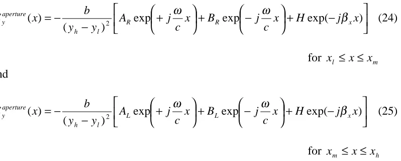
where the mid point of the line is at xm =(xl +xh)/2. Combining these boundary conditions with Equations 14-17 yields the following matrix equation:

(11)

The coefficients A , L B , L A andR B can now be found by a simple matrix inversion, and the R

solution for the voltage on the two wire line in Figure 3 is defined by Equations 14 and 15. The field Eaperture(x)

y in the two-wire line is given by −VL/RHS(x)/(yh −yl). As before, this field is

[image:11.595.79.478.213.373.2]

multiplied by a factor b/(yh −yl) to account for the extended vertical height b of the box in Figure 1. The field in the aperture, in the absence of the rest of the box in the region z>0, is thus given by

      _₊ ₋     − +      + − −

= exp exp exp( )

) (

)

( ₂ x H j x

c j B x c j A y y b x

E _R _R _x

l h aperture y β ω ω (24)

for xl ≤x≤xm

and       _₊ ₋     − +      + − −

= exp exp exp( )

) (

)

( ₂ x H j x

c j B x c j A y y b x

E _L _L _x

l h aperture y β ω ω (25)

for xm ≤x≤xh

This aperture field is of course modified by the reaction of energy that enters and exits the rest of the box in the region z >0 in Figure 1. Sections 4 and 5 explain how this is dealt with in terms of modal analogous transmission line theory, and how this leads to the entire field problem being expressed in terms of an equivalent circuit problem.

4 Excitation of modes in infinitely long waveguide by aperture field.

Equivalent circuit representation and the principle of reciprocity

4.1 Excitation of modes by aperture field

For an infinitely long waveguide, or alternatively an absorbing wall in the plane z=d in Figure 1, the fields E and _y E inside the waveguide can be expressed as a sum of forward travelling _x

TE and TM modes i.e.

(12)

(

)

(

)

∑∑

∞ = ∞ = ∞ = ∞ =                   − +                   − − = 1 1 0 1 sin cos exp sin cos exp ) ( m n mn TM fmn m n mn TE fmn x b y n a x m a m z C b y n a x m b n z C E π π π γ π π π γ r (27)

where γ_mn is given by

(

2 2

)

0

0ε ω ω

µ

γmn = c − (28)

2 2 0 0 2       +       = b n a m c π π ε µ

ω (29)

The individual coefficients C are as yet unknown, but as we shall see below, with some approximations they can ultimately be expressed in terms of the aperture field.

If we evaluate

0 ) ( = = z y y E

E r from Equation 26 in the plane z=0, multiply by 

     b y uπ cos

where u=0,1,2,.... and integrate with respect to y from y=0 to y=b we obtain

(

)

(

)

∑

∫

∞ = ∞ = = +             + +             =       1 0 1 0 0 0 1 2 sin 1 2 sin cos m u TM fmu m u TE fmu b z y b a x m b u C b a x m a m C dy b y u E δ π π δ π π π (30)

where δu0 is the Kronecker-delta symbol, equal to unity for u=0 and zero for u≥1.

We now require

0 =

z y

E to equal zero for 0≤ y≤ y_l and y_h ≤ y≤b (zero tangential electric field

at a metal surface). We further assume that

0 =

z y

E in the aperture is in fact independent of y.

This will be a very good approximation if the slot is narrow, or at least if the width g =y_h −y_l

of the slot is small compared to a wavelength of radiation. Under these assumptions, we can evaluate the left hand side of Equation 30 to give

u actual ap y y y actual ap

y dy E x N

b y u x E h l × =      

∫

cos ( )

) ( _ _ π (31) where     ≥             −       = − = 1 sin sin 0 u b y u b y u u b u y y

N h l

l h

u π π

π

(13)

Combining Equations 31 and 30, we obtain

(

)

∑

∞ = +             _      +       = 1 _ 1 2 sin ) ( m uo TM fmu TE fmu actual ap y u b a x m b u C a m C x E

N π π π δ (33)

Equation 33 holds for each value of u. Hence putting u=0 results in

∑

∞ =            = 1 0 0 _ sin ) ( m TE fm actual ap y a x m a m C N b x

E π π (34)

Putting u=n≥1 into Equation 33 results in

∑

∞ =                  +       = 1 _ sin 2 ) ( m TM fmn TE fmn n actual ap y a x m b n C a m C N b x

E π π π (35)

Clearly the aperture field Eyap_actual(x) has a unique Fourier series expansion involving only sine

functions, so that we can equate the coefficients of 

     a x mπ

sin in Equations 34 and 35. Thus, for

,.... 3 , 2 , 1 =

m and n=1,2,3,....

            +       =       b n C a m C N a m C N TM fmn TE fmn n TE fm π π π 2 1 1 0 0 (36)

This provides one linear relationship between the coefficients C. A second linearly independent relationship can be found by considering the slot as a transmission line, supporting transverse electromagnetic (TEM) waves. Once again, this is a good assumption providing the gap g is small compared to a wavelength. In this case, we can approximate the field E in the aperture to x

be zero, since it becomes a longitudinal component of field as far as the slot/transmission line is concerned. Combined with the boundary condition of zero tangential field E everywhere else x

on the plane z =0 (due to the presence of the metal box), we can require the field E to equal _x

zero everywhere in the plane z=0. This is only possible in Equation 27 if we set each

coefficient of 

           b y n a x

mπ π

sin

cos equal to zero. Thus we obtain, for m=0,

0 sin

1

0 =

          

∑

∞ = b y n b n C n TE n f π π (37) Requiring 0 0 = TE n f

(14)

(This is also an intuitive result for a slot illuminated by a field Eyinc). For m=1,2,3,.... and ,.... 3 , 2 , 1 =

n we must also have

0 =       +       − a m C b n

C TMfmn

TE fmn

π π

(39)

Equations 39 and 36 are two linearly independent relationships which allow each of CTEfmn and TM

fmn

C to be expressed in terms of TE fm C ₀ i.e.

        _                − =         − 0 2 ₀ 0 1 TE fm n TM fmn TE fmn C a m N N a m b n b n a m C C π π π π π (40)

Finally, given the actual aperture field Eap_y _actual(x), the coefficients CTE_fm₀ may be found from

Equation 34, by multiplying by 

     a x uπ

sin and integrating with respect to x from x=0 to x=a.

The result is (on replacing the dummy integer u by m),

dx a x m x E a a m C N b h l x x actual ap y TE

fm

∫



     =     

 π π

sin ) ( 2 _ 0 0 (41)

Equations 41 and 40 allow all coefficients CTEfmn, TM fmn

C to be deduced. These may then be inserted into Equations 26 and 27 to yield the entire field structure for E and y E inside the x

waveguide of Figure 1, in the presence of an absorbing wall at z=d. It remains to find a method for estimating the field Eyap_actual(x) in the aperture.

4.2 Equivalent circuit representation and the principle of reciprocity

It is tempting at this point to set the unknown aperture field Eap_y _actual(x) in Equation 41 to the

previously calculated Eyaperture(x) of Equations 24 and 25. However, this will not yield correct

(15)

We can however use the field Eyaperture(x) of Equations 24 and 25 as a starting point to estimate the excitation of the different modes by a plane wave incident on the box from free space. We can then use the principle of reciprocity to estimate the reaction of the modes back on to free space, and at the same time get some measure of the extent of mode coupling that would take place if a particular mode i were incident on the aperture from within the box, resulting in a multitude of modes being reflected back into the box. The procedure is implemented by an equivalent circuit where each waveguide mode is represented by an analogous transmission line with a characteristic impedance equal to the impedance of the transverse ratio of E and H fields for the mode. The connection between the mode amplitude and the amplitude of the voltage/current waves on the analogous transmission line is made quantitative by insisting that the power flow down the analogous transmission line is equal to the power flow down the waveguide.

Ω

377

FS

I

source

V

) 1 (

loop

ε

) 2 (

loop

ε

) ( N

loop

ε

+ + + +

_ _ _

_ (1)

wg

V

) 2 (

wg

V

) 1 (

wg

I

) 2 (

wg

I

) 1 ( ) 1 ( ) 1 (

)

tanh( T

c d Z

Z γ =

) 2 ( ) 2 ( ) 2 (

)

tanh( _T

c d Z

Z γ =

+ +

_

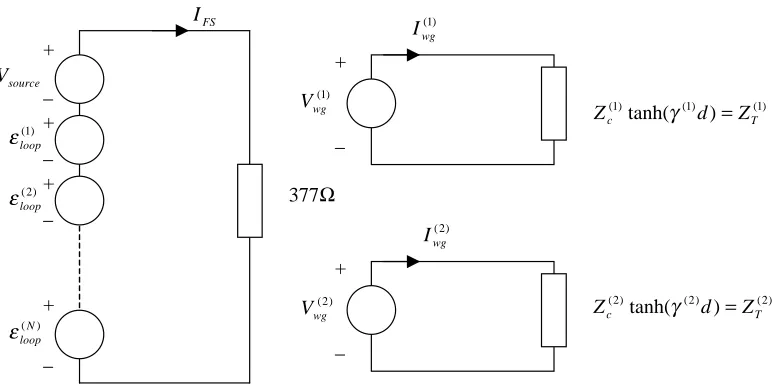
[image:15.595.103.490.314.506.2]

Figure 4. Equivalent circuit for experimental set up in Figure 1.

Figure 4 shows the equivalent circuit model representing the physical problem of Figure 1. For simplicity, only two waveguide modes are shown. The incident electric field in Figure 1 is represented by Vsource, which is responsible for the main part of the current IFS flowing through

the 377Ω resistor (representing the impedance ZFS of free space). Each of the voltage sources

) (n

wg

V at the start of the analogous transmission lines is made to depend on the current IFS, such

(16)

via a transimpedance ZTrans(n) such that FS n Trans n

wg Z I

V( ) = ( )

. The value of this transimpedance is also derived in Section 4.3. This type of coupling can also be described in terms of a mutual inductance M such that jωM =ZTrans(n) , and is the magnetic analogue of electric field coupling in

terms of a mutual capacitance C [14]. The problem is formulated in terms of contolled voltage sources (as opposed to controlled current sources) because in the absence of any mode coupling, the slot or aperture appears as a short circuit to any modes or voltage waves incident on the slot from within the waveguide. This is a reasonable approximation to make if the slot is narrow. If controlled current sources were used, the slot would appear as an open circuit, which is not what the physical problem looks like (except possibly for very large apertures).

The principle of reciprocity can be taken into account by including reactive e.m.f.s (n)

loop

ε in the ‘free space’ circuit, where each e.m.f. represents the reaction of a particular mode into free space. Thus if Vwg ZTransIFS

) 1 ( ) 1 ( =

, we can take the principle of reciprocity into account by setting

) 1 ( ) 1 ( ) 1 (

wg Trans loop =Z I

ε , where Iwg(1) is the current through

) 1 (

wg

V . Note that this mechanism guarantees that mode coupling will take place in the aperture: An incident mode i from within the cavity will excite εloop(i) , causing current to flow through the 377Ω resistor and exciting all other

forward travelling modes (including mode i itself).

The following sections outline the derivation of the expressions for ( n)

Trans

Z (TE and TM modes) and Vsource, and describe how the fields internal to the box may be derived from knowledge of the

terminal voltages (n)

wg V .

4.3 Derivation of

(n)

Trans

Z

and

Vsource

4.3.1 TE modes

From Equation 26, the contribution of the forward travelling TEmn mode to the electric field E y

in the plane z=0 of Figure 1 is given by

                  =

= _b

y n a

x m a

m C Ey _z TEfmn

π π

π

cos sin

0 (42)

By equating the power transferred by the TEmn mode with the power transferred down its

analogous transmission line, the individual forward and reverse fields can be related to the individual forward (V ) and reverse (f0

0

r

V ) voltages on the analogous transmission line by

) exp(

0 0

z sf

j Z

V

E _x _mn

mn TE mn f for

y _γ γ

ωµ ₋

−

(17)

) exp( 0 0 z sf j Z V

E _x _mn

mn TE mn r rev

y _γ γ

ωµ ₊

−

= (44)

where [14]                                 +       = b y n a x m a m b n a m

fx mn

π π π π π γ cos sin 2

2 (45)

2 1 2     = mn TE mn Z s

α (46)

(

)(

)

(

)(

)

        − +       + + −                     +       −

= 0 0

2 0 0 2 2 2 2 0 1 1 1 1

8 m n m n

mn mn b n a m ab b n a m j δ δ π δ δ π π π γ ωµ α (55)

Equating (42) and (43) in the plane z=0 results in

              +       − = 2 2 0 0 b n a m s j Z C V TE mn TE fmn f π π

ωµ (48)

Here TE mn

Z is the characteristic impedance ( n)

c

Z (see Figure 4) of the analogous transmission line and is given by

mn TE mn j Z γ ωµ0

= (49)

We first separate out the forward and reverse waves by assuming that the plane z=d in Figure 1 is perfectly absorbing, or alternatively that the waveguide dimension d is infinite. This results in forward travelling waves only, and for the case of an infinitely long waveguide effectively means that we have terminated each of the analogous transmission lines in its characteristic impedance Z_c(n). Later we shall reintroduce the short circuit in the plane z =d and let the circuit we have derived deal naturally with any reflections that occur from the back wall. The advantage of this approach is that the rectangular cavity can then indeed be treated as a superposition of analogous transmission lines, allowing existing ILCM techniques to model the presence of a monopole or loop inside the cavity (e.g. [13][14]).

For the experimental set up in Figure 1, βx =βy =0. From Equations 4-7, 23-25, 32, 40 and 41

(18)

the initial assumption that E _ (x) Eyaperture(x)

actual ap

y = , in the absence of any box in the region

0

>

z in Figure 1. We note here that for an incident plane wave travelling in a given direction bˆ with a given polarization, the field Hincz in Equation 6 is directly proportional to

inc y

E with a known constant of proportionality. We can therefore write

inc y TE

fmn k E

C = 1 (50)

inc y TM

fmn k E

C = ₂ (51)

where k and 1 k are known constants. 2

Combining Equations 48 and 50, we obtain

inc y TE

mn

f k E

b n a

m s j

Z

V ₁

2 2

0 0

    

  

      +       −

= π π

ωµ (52)

It remains to relate Eyinc to IFS, in the absence of any reaction from the analogous transmission

lines into free space (i.e. we set all the e.m.f.s εloop(n) =0 in Figure 4). In this case, the peak power in the incident wave that impinges on the box for a yˆ polarised wave travelling in the zˆ direction is given by

FS FS FS

inc y

Z I ab Z

E

P 2

2

) ( ) (

= ×

= (53)

or

ab Z

E I

FS inc y

FS = (54)

Clearly this requires a source voltage (in the absence of any reactive e.m.f.s)

ab E

Vsource = incy × (55)

Finally, from Equations 54 and 52 we can write our forward travelling voltage wave in an infinitely long waveguide/analogous transmission line as

FS FS TE

mn

f I

ab Z k b n a

m s j

Z

V 1

2 2

0 0

    

  

      +       −

= π π

(19)

0

f

V is of course equal to one of the voltage sources (n)

wg

V in Figure 4, and represents the excitation of the forward travelling TEmn mode.

Equation 56 defines our transimpedance ZTrans(n) for TE modes. It is given by

ab Z k b n a m s j Z Z Z FS TE mn TE Trans n Trans mn 1 2 2 0 ) (               +       − =

= π π

ωµ (57)

The value of Vsource is given by Equation 55.

4.3.2 TM modes

A similar treatment for TM modes results in a transimpedance

ab Z k b n a m u Z Z FS mn TM Trans n Trans mn 2 2 2 ) ( 1               +       ′ − =

= π π

γ (58)

where

(

)

2

1 2 1 TM mn mnZ u α′ =

′ (59)

8 2 2 0 ab b n a m j mn mn               +       − = ′ π π γ ωε

α (60)

0

ωε γ

j

ZTM mn

mn = (61)

mn

γ and k are defined in Equations 28 and 51 respectively. The forward travelling voltage for 2

a TM mode in the presence of an infinitely long waveguide is therefore given by

FS n Trans

f Z I

V0 = ( ) (62)

where ZTrans(n) is given by Equation 58.

0

f

V is of course set equal to one of the voltage sources

) (n

wg

(20)

5 Completion of the circuit and the reintroduction of the reflecting

back wall. Reconstruction of field in cavity.

5.1 Reintroduction of reflecting back wall

Having obtained our values of Z_Trans(n) for TE modes (Equation 57) and TM modes (Equation 58), and knowing what value to assign to Vsource for a given

inc y

E (Equation 55), we can complete our circuit so as to model the original problem of Figure 1. As indicated in Section 4.2, the principle of reciprocity is taken into account by including a reaction e.m.f. ε_loop(n) in the ‘free space’ circuit

of Figure 4 for every mode excitation voltage (n)

wg

V , such that

FS n Trans n

wg Z I

V( ) = ( ) (63)

) ( ) ( )

( n

wg n Trans n

loop =Z I

ε (64)

The conducting wall in the plane z=d can easily be reintroduced. All that is required is to alter the ‘absorbing’ terminating characteristic impedances Zc(n) for the analogous transmission lines

(which have been implicitly assumed in the derivations of Section 4.1) to the impedances of the short-circuited sections of transmission line seen by the various Vwg(n). These impedances are

given by Z( ) Zc(n) tanh( (n)d)

n

T = γ , as indicated in Figure 4. The effect of this is to reflect current

into the dependent voltage sources Vwg(n), causing additional excitation of the e.m.f.s

) (n

loop ε , via Equation 64. This in turn alters IFS and causes

) (n

wg

V itself to change via Equation 63. The circuit solution of Figure 4 effectively describes what happens under steady state conditions, once all these transient effects have died down. Note that the resulting actual field Eapy _actual(x)

in the aperture is no longer equal to the initial field Eyaperture(x) of Equations 24 and 25, since the modes have been allowed to couple and therefore influence each other.

5.2 Reconstruction of the field inside the cavity

The circuit of Figure 4 may be solved for the voltages Vwg(n) using modified nodal analysis [21],

noting that simple nodal analysis is inadequate because of the presence of dependent voltage sources. Alternatively, a simple algebraic manipulation of the circuit equations for Figure 4 with

N modes yields the result,

N n

I Z

V FS

n Trans n

wg 1,....

) ( )

( = =

(65)

(21)

[ ]

FS N n n T n Trans source FS Z Z Z V I −                 − =

∑

=1 ) ( 2 ) ( (66)

In the presence of a conducting wall in the plane z=d, it is a simple matter to decompose the terminal voltages Vwg(n) into forward (

0

f

V ) and reverse (V ) travelling waves: r0

) 2 exp(

1 ( )

) ( 0 d V V _n n wg f γ − −

= (67)

) 2 exp(

1 ( )

) ( 0 d V V _n n wg r γ + −

= (68)

For TE modes these values of V and f0

0

r

V may be used in conjunction with Equations 43 and 44

to reconstruct the total field E at any point inside the box due to TE modes only. For TM y

modes, the field E at any point inside the box can be found from _y

) exp( 0 z g u V

E f y mn

for

y =− ′ −γ (69)

) exp( 0 z g u V

E r y mn

rev

y =− ′ +γ (70)

                                +       = b y n a x m b n b n a m

gy mn

π π π π π γ cos sin 2

2 (71)

(The quantity u′ is defined in Equations 59-61). By summing the total fields due to forward and reverse waves for TE and TM modes, the overall total field EToty (r) at any point inside the box may be calculated. The shielding effectiveness SE at that point is then given by

        − = _inc y Tot y E E ( ) log 20 ) ( SE 10 r

r (72)

(N.B. Other definitions for SE may be used since we are totally ignoring E and x E , though z

(22)

6 Results

In this section the results of the ILCM model presented in Sections 2-5 are compared with results of numerical modelling using the transmission line matrix (TLM) method. The TLM simulations were performed using a 5mm grid. Various cases of apertures in boxes are considered, and these appear in Table 1. The aim was to consider a reasonably varied assortment of box sizes, aperture sizes and positions and field observation points, without producing an excessive amount of data. In all cases the incident field consists of a yˆ polarized wave travelling in the zˆ direction, as in Figure 1.

Case No.

a

(cm)

b

(cm)

d

(cm) l

x

(cm)

l y

(cm)

Slot length

l h x x −

(cm)

Slot height

l h y y −

(cm)

) , , (x y z obs

r (cm) Comments on slot

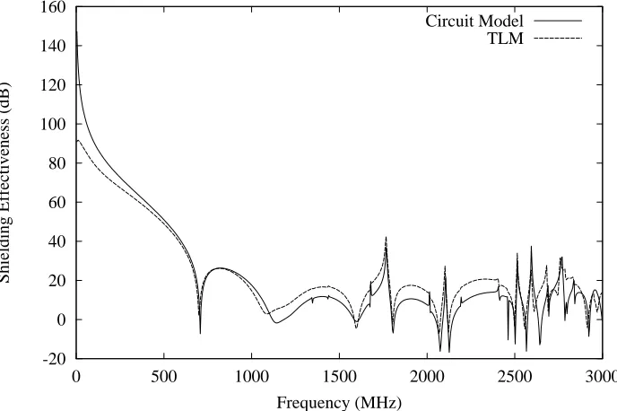
1 48.5 12.0 48.5 1.5 10.0 45.5 1.0 (24.25,11.75,42.25) Near lid 2 30.0 12.0 30.0 0.0 5.75 30.0 0.5 (15.0,12.0,14.75) Full width 3 30.0 12.0 30.0 0.0 11.5 30.0 0.5 (15.0,12.0,15.25) Near lid 4 30.0 12.0 30.0 10.0 6.0 10.0 0.5 (14.75,11.75,15.25) Central 5 30.0 12.0 30.0 0.0 6.0 15.0 0.5 (14.75,11.75,15.25) Off centre 6 20.0 10.0 30.0 2.0 1.0 8.0 1.0 (4.75,4.75,22.25) Off centre 7 20.0 16.0 20.0 10.0 4.0 8.0 8.0 (4.75,8.25,14.75) Square 8 20.0 16.0 20.0 10.0 4.0 8.0 1.0 (4.75,8.25,14.75) Off centre 9 30.0 12.0 30.0 10.0 6.0 10.0 0.5 (22.25,6.75,28.25) Central (as 4) 10 30.0 12.0 30.0 10.0 6.0 10.0 0.5 (22.25,6.75,15.25) Central (as 4)

Table 1. The various cases considered for comparison of the ILCM circuit model with TLM. a, b and d are the box dimensions, while the aperture dimensions and position are determined by

l

x , x , _h y and _l y (see Figure 1). _h r_obs(x,y,z) is the position inside the box where the field E _y

is sampled in both the circuit model and TLM.

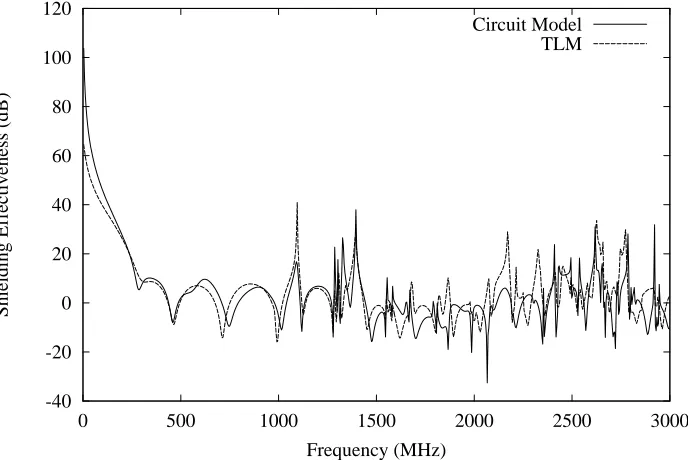
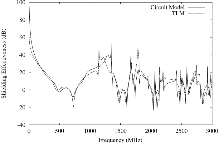
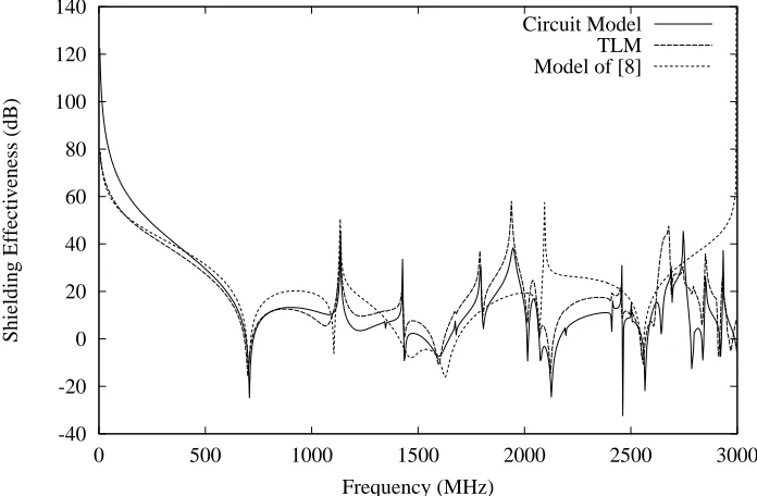
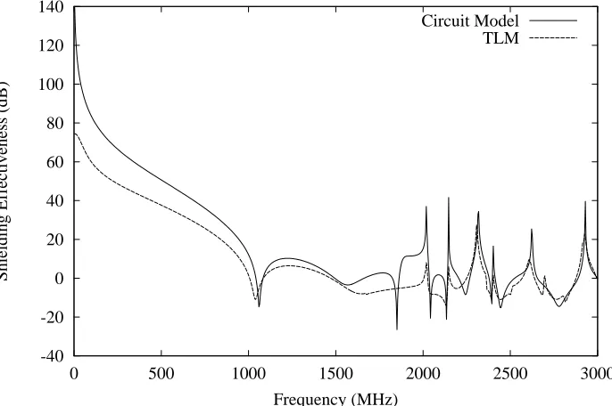
The circuit model and TLM values for SE as defined in Equation 72 are compared for the ten different cases in Figures 5-14. With the exception of case 7 in Figure 11, the agreement is generally seen to be excellent, both qualitatively and quantitatively. The upper frequency range considered is 3GHz, where many higher order modes are present. Simple TE10 models such as

[8] and [9] would be totally inadequate at such frequencies (see for example the result of the model in [8] plotted in Figure 8). In contrast, there is seen to be little deterioration in accuracy even at such high frequencies for the current model. Moreover, the model is able to cope with significantly off centre slots, something not possible with other models.

It is seen in Figure 11 (case 7) that the agreement with TLM is relatively poor (though curiously this is not true at high frequencies). This might be expected for this particular aperture since the aperture is in fact square, and cannot therefore be considered ‘slot’ like. The concept of the aperture forming a transmission line is likely to break down in this case, and the initial assumption of zero E field in the aperture (see Figure 1) is unlikely to be a good _x

(23)

In Figures 6-14 all modes up to m=5, n=5 are considered, a total of 55 modes (ignoring TE0n

modes where CTE_f₀_n =0 from Equation 38). Many of the higher order modes will be evanescent for much of the frequency range below 3GHz, and this is reflected by the fact that γmn is real.

This does not however cause any difficulties with the theory, which can readily accommodate evanescent modes. The choice of m=5, n=5 for the upper limit on modes ensures that all propagating modes below 3GHz are included in the ILCM model in Figures 6-14. For larger boxes and/or higher frequencies it is necessary to increase the limits on m and n, and this is easily implemented in the ILCM model presented here. For example, for the large box in case 1 of Figure 5, all propagating modes below 3GHz (and a lot of extra evanescent modes) are taken into account by setting an upper limit of m=9, n=9. As a general rule, it is best to at least include all propagating modes up to the highest frequency of interest (in our case 3GHz), though the inclusion of some higher order evanescent modes can improve the results further (see for example [14]).

Table 2 summarises the statistics for the agreement between the circuit model and TLM in Figures 5-14. The normalised cross correlation coefficient ρdB(0) is defined here as

{

∫

}

∫

∞ +

∞ −

∞ +

∞ − +∞

∞

− −

=

ω ω ω

ω

ω ω ω ω ω

ρ

d S d S

d S

S

) ( )

(

) (

) ( )

(

2 2 2

1

0 2

1 0

dB (73)

and is always less than or equal to unity. S and ₁ S are the SE responses in dB. If ₂ S₁(ω)and )

(

2 ω

S are identical then ρdB(0)=1. (Indeed, ρdB(0)=1 even if S1(ω)=C0S2(ω) for some

arbitrary constant C , so that 0 ρdB(0) gives some measure of the similarity of the shapes of the

responses S₁(ω)and S₂(ω) in dB). Excluding case 7, the overall rms difference between the curves in Figures 5-14 is 7.70dB, with a mean absolute error of 5.55dB and a correlation coefficient ρ_dB(0)=0.9440. On an intuitive visual examination of the curves, it is clear that the agreement is very good. It is noted from Section 2.1 that the agreement in every single case in Table 2 is made worse by assuming the quasi-static impedance of [19] for the transmission line ‘slot.’ The overall rms difference in the latter case is 9.59dB, with a mean absolute difference of 7.08dB.

Figure 15 illustrates the level of accuracy that can reasonably be expected from the TLM technique when compared to experimental measurements. The experiment carried out here was for the scenario illustrated in case 1 of Table 1. Irradiation was via a horn antenna inside an anechoic chamber, with a monopole of length 2.5cm and diameter 1mm acting as a detector inside the box. The shielding effectiveness of the box at the location described in Table 1 was deduced from two measurements of s , with the network analyser output feeding the horn ₂₁

(24)

below which SE could not be reliably measured (i.e. the shielded measurement was below the noise floor). The rms difference between the experimental results and TLM in Figure 15 is 7.84dB, with a mean absolute error of 5.98dB and a correlation coefficient ρ_dB(0)=0.5772. Thus the agreement with experiment exhibited by TLM is of a similar (or worse) level to the agreement of TLM with the ILCM model in Table 2. (The agreement of the ILCM model with this particular experiment is a little worse, being characterised by an rms difference of 10.10dB, mean absolute difference of 7.91dB and a correlation coefficient of just ρdB(0)=0.2197). Due to the highly resonant nature of the curves and the sensitivity of the measurements to position, an rms error of 7 or 8dB is not unreasonably high: Two resonant curves which are slightly displaced will exhibit a large rms error whilst being both qualitatively and quantitatively in good agreement.

The time taken for the circuit model to reach a solution is much smaller than that taken by the numerical method of TLM. The data in each of Figures 5-14 consist of 750 frequency points separated by approximately 4MHz, with TLM taking four hours and twenty minutes to reach solution (Pentium III, 750MHz). In contrast, on the same computer the circuit model running in MATLAB (a relatively slow interpreted language) took just 30 seconds to reach solution (except for Figure 5 with the extra modes), a factor of 500 times faster. Indeed, when compiled in C++ the circuit model provides the same data in approximately 2 seconds. Combined with the 2 seconds or so required to run the subsidiary NEC simulation, this represents a speed of solution 3900 times faster than TLM.

-40 -20 0 20 40 60 80 100 120

0 500 1000 1500 2000 2500 3000

Shielding Effectiveness (dB)

Frequency (MHz)

[image:24.595.132.476.415.645.2]

Circuit Model TLM

Figure 5. Comparison of the shielding effectiveness predicted by the ILCM circuit model with the numerical prediction of TLM for the box, aperture size and position indicated in Case 1 of

(25)

-20 0 20 40 60 80 100

0 500 1000 1500 2000 2500 3000

Frequency (MHz)

[image:25.595.129.475.111.340.2]

Circuit Model TLM

Table 1.

-40 -20 0 20 40 60 80 100

0 500 1000 1500 2000 2500 3000

Frequency (MHz)

Circuit Model TLM

[image:25.595.127.478.411.640.2]

(26)

-40 -20 0 20 40 60 80 100 120 140

0 500 1000 1500 2000 2500 3000

Frequency (MHz)

[image:26.595.128.476.113.341.2]

Circuit Model TLM Model of [8]

Figure 8. Comparison of the shielding effectiveness predicted by the ILCM circuit model with the numerical prediction of TLM for the box, aperture size and position indicated in Case 4 of Table 1. The prediction of the simple TE10 model of [8] is also shown; this is clearly seen to be

inadequate at frequencies above 1GHz.

-40 -20 0 20 40 60 80 100 120

0 500 1000 1500 2000 2500 3000

Frequency (MHz)

Circuit Model TLM

[image:26.595.134.476.422.654.2]

(27)

-40 -20 0 20 40 60 80 100 120 140 160

0 500 1000 1500 2000 2500 3000

Frequency (MHz)

[image:27.595.129.476.113.340.2]

Circuit Model TLM

Table 1.

-40 -20 0 20 40 60 80 100 120 140

0 500 1000 1500 2000 2500 3000

Frequency (MHz)

Circuit Model TLM

[image:27.595.132.475.411.639.2]

(28)

-40 -20 0 20 40 60 80 100 120 140

0 500 1000 1500 2000 2500 3000

Frequency (MHz)

[image:28.595.128.476.113.340.2]

Circuit Model TLM

Table 1.

-20 0 20 40 60 80 100 120 140 160

0 500 1000 1500 2000 2500 3000

Frequency (MHz)

Circuit Model TLM

[image:28.595.131.475.411.640.2]

(29)

-40 -20 0 20 40 60 80 100 120 140

0 500 1000 1500 2000 2500 3000

Frequency (MHz)

[image:29.595.128.475.113.340.2]

Circuit Model TLM

Table 1.

Case No. Rms difference (dB) Mean absolute difference (dB)

) 0 (

dB

ρ

1 8.10 5.84 0.8599

2 6.62 4.59 0.9275

3 7.58 5.36 0.9161

4 8.49 6.41 0.9455

5 7.69 5.61 0.9499

6 7.70 4.85 0.9831

7 11.52 8.90 0.9763

8 7.08 5.12 0.9821

9 7.63 5.80 0.9781

10 8.24 6.38 0.9536

Overall (Excluding case 7)

7.70 5.55 0.9440

Table 2. Summary of agreement of circuit model with TLM. The table shows the rms difference, mean absolute difference and correlation coefficient for the shielding effectiveness curve predictions of the circuit model and TLM between 4MHz and 3GHz for the ten different

[image:29.595.68.500.429.629.2]

(30)

-20 0 20 40 60

0 500 1000 1500 2000 2500 3000

Frequency (MHz)

[image:30.595.128.475.114.341.2]

Experiment TLM

Figure 15. Comparison of the shielding effectiveness predicted by TLM with experimental results for the box, aperture size and position and observation point indicated in Case 1

of Table 1.

7 Conclusions

An intermediate level circuit model (ILCM) has been developed to model the plane wave excitation of a rectangular box containing a rectangular aperture. The model has been developed in such a way that existing ILCM techniques for modeling the presence of elements such as dipoles, monopoles, loops and transmission lines inside the box can easily be incorporated into the circuit (though for simplicity we have been concerned only with an empty box here). The ILCM model can incorporate as many higher order modes as are necessary to adequately describe the box excitation at the highest frequency of interest. Both propagating and evanescent modes are permitted. Although the model is best suited to ‘slot’ type apertures, where the slot height is a small fraction of the slot length (e.g. less than 12%), the aperture may be positioned anywhere in the front face of the box, and is not limited to the central position in height and width. The model takes into account both inter-mode coupling and reradiation into free space.

(31)

effectiveness. Indeed, it is known that the latter features can be highly sensitive to position and therefore to the spatial resolution used in the TLM simulations. An rms difference of 7 or 8 dB between the ILCM model and TLM is therefore not unreasonably high. Indeed, this is the level of agreement that can be expected between a numerical TLM simulation and an experimental measurement, as illustrated in Figure 15. The main problem lies in the fact that two resonant peaks that are slightly displaced can lead to a large rms difference, when in reality there is good qualitative and quantitative agreement between the two curves, which is evident from visual inspection.

Acknowledgments

The authors wish to acknowledge that this work was made possible by support and funding from BAE Systems. Many thanks to Ian MacDiarmid.

References

[1] R.F. Harrington and J.R. Mautz, “Characteristic modes for aperture problems,” ,” IEEE

Trans. Microwave Theory Tech., vol. 33, no. 6, pp. 500-505, Jun. 1985.

[2] Y. Xingchao, R.F. Harrington and J.R. Mautz, “The pseudo-image method for computing the electromagnetic field that penetrates into a cavity,” Archiv fur Elektronik und

Uebertragungstechnik, vol. 41, no. 5, pp. 307-317, Sept.-Oct. 1987.

[3] T. Wang, R.F. Harrington and J.R. Mautz, “Electromagnetic scattering from and transmission through arbitrary apertures in conducting bodies,” IEEE Transactions on Antennas

and Propagation, vol. 38, no. 11, pp. 1805-1814, Nov. 1990.

[4] R.F. Harrington and J.R. Mautz, “Electromagnetic coupling through apertures by the generalized admittance approach,” Computer Physics Communications, vol. 68, pp. 19-42, Nov. 1991.

[5] S.V. Georgakopoulos, C.R. Birtcher, and A. Balanis, “HIRF penetration through apertures: FDTD versus measurements,” IEEE Trans. Electromagn. Compat., vol. 43, pp. 282-294, Aug. 2001.

[6] P. Sewell, J.D. Turner, M.P. Robinson, D.W.P. Thomas, T.M. Benson, C. Christopoulos, J.F. Dawson, M.D. Ganley, A.C. Marvin, and S.J. Porter, “Comparison of analytic, numerical and approximate models for shielding effectiveness with measurement,” IEE Proc. Sci. Meas.

Technol., vol. 145, no.2, pp. 61-66, Mar. 1998.

[7] W. Wallyn, D. De Zutter, and H. Rogier, “Prediction of the shielding and resonant behaviour of multisection enclosures based on magnetic current modeling,” IEEE Trans.