Modelling of laser forming at macro and micro scales

M

ACRO AND

M

ICRO

S

CALES

Thesis submitted in accordance with the requirements of the University of Liverpool for the degree of Doctor in Philosophy

by

J

D

G

Primary supervisor: Prof. Ken Watkins Secondary supervisor: Dr. Geoff Dearden

Laser Engineering Group School of Engineering University of Liverpool

LIST OF PUBLICATIONS

Journal Papers

1. Griffiths J., Edwardson S.P., Dearden G., Watkins K.G., Finite Element modelling of laser forming at macro and micro scales, Physics Procedia, Vol 5, pp 371-380 (2010) 2. Edwardson S.P., Griffiths J., Dearden G., Watkins, K.G., Temperature gradient

mechanism: Overview of the multiple pass controlling factors, Physics Procedia, Vol 5, pp 53-63 (2010)

3. Edwardson S.P., Griffiths J., Edwards K.R., Dearden G., Watkins K.G., Laser forming: overview of the controlling factors in the temperature gradient mechanism, Proceedings of the Institution of Mechanical Engineers, Part C: Journal of Mechanical Engineering Science, Vol 224, 5, pp 1031-1040 (2010)

4. Griffiths J., Edwardson S.P., Boegelein T., Prandina M., Dearden G., Watkins K.G., Finite Element Modelling of the Laser Forming of AISI 1010 Steel, Lasers In Engineering, Vol 22, 5, pp 401-412, (2011)

5. Edwardson S.P., Griffiths J., Dearden G., Watkins, K.G., Towards Controlled Three-Dimensional Laser Forming, Lasers in Engineering, Vol 22, 5, pp 393 (2011)

6. Griffiths J., Edwardson S.P., Dearden G., Watkins K.G., Thermal Laser Micro-Adjustment Using Picosecond Pulse Durations, Applied Surface Science, Vol 258, 19, pp 7639–7643 (2012)

Conference Papers

1. Prithwani, I., Otto, A., Schmidt, M., Griffiths, J., Watkins, K. G., Edwardson, S. P., Dearden, G., “Laser Beam Forming of Aluminium Plates under Application of Moving Mesh and Adapted Heat Source”, Proceedings of the Fifth International WLT-Conference on Lasers in Manufacturing 2009, Munich, June 2009

2. Griffiths, J., Edwardson, S. P., Dearden, G., Watkins K. G., “Finite Element Modelling of the Laser Forming of AISI 1010 Steel”, Proceedings of the 36th international MATADOR conference, Manchester, 2010

3. Edwardson, S. P., Griffiths, J., Dearden, G., Watkins K. G., “Towards Controlled 3D Laser Forming”, Proceedings of the 36th international MATADOR conference, Manchester, 2010

5. Griffiths, J., Edwardson, S. P., Dearden, G., Watkins K. G., “Short Pulse Thermal Laser Microforming Technique”, Proceedings of IWOTE’2011, Bremen, Germany, 2011

6. Griffiths, J., Edwardson, S. P., Dearden, G., Watkins K. G., “Laser Micro Adjustment Using Ultra Short Pulses”, Proceedings of ICALEO’2011, Florida, USA, 2011

7. Griffiths, J., Edwardson, S. P., Dearden, G., Watkins K. G., “Modeling of Real Temporally Variant Beam Shapes in Laser Materials Processing”, Proceedings of ICALEO’2011, Florida, USA, 2011

8. Griffiths, J., Edwardson, S. P., Dearden, G., Watkins K. G., “Thermal Laser Micro-Adjustment Using Ultra-Short Pulses”, Proceedings of the 37th international MATADOR conference, Manchester, 2012

Press Articles

DECLARATION

I hereby declare that all of the work contained within this thesis has not been submitted for any other qualification.

Signed: _________________________________

ABSTRACT

Laser forming (LF) offers industry the promise of controlled shaping of metallic and non-metallic components in prototyping, correction of design shape or distortion and precision adjustment applications. In order to fulfil this promise in a manufacturing environment the process must have a high degree of controllability, which can be achieved through a better understanding of its underlying mechanisms.

The work presented in this thesis is primarily concerned with the use of modelling of the LF process at macro and micro scales as a means of process development.

At the macro scale, finite element (FE), finite difference (FD) and analytical modelling were used to gain a better understanding of the complex interrelation between the various process parameters for specific geometries, reducing the need for extensive empirical investigations. A particular focus of the investigation was ascertaining which of these parameters influenced the fall off in bend angle per pass in multiple pass LF, along with the magnitude of their influence.

The development of a full thermal-mechanical model of the LF process is detailed, as well as its application in a feasibility study into the forming of square section mild steel tubes for the automotive industry. Using this model, experimental observations were rationalized and novel scan strategies were developed which optimized the efficiency and accuracy of the process, something hitherto not possible using empirical methods alone.

CONTENTS

LIST OF PUBLICATIONS

...

Journal Papers... iii

Conference Papers... iii

Press Articles ... iv

DECLARATION

...

...

...

...

...

...

GLOSSARY OF TERMS

...

INTRODUCTION...1

Research Objectives ... 2

Thesis Structure... 3

CHAPTER 1...5

LITERATURE REVIEW

...5

1.1 The Laser Heating Process... 5

1.2 Laser Forming Mechanism Overview ... 8

1.2.1 Temperature gradient mechanism (TGM) ... 9

1.2.2 Buckling mechanism (BM) ... 13

1.2.3 Upsetting mechanism (UM) ... 14

1.2.4 Effect of process parameters... 14

1.3 Metallurgy of Steels during Laser Forming ... 16

1.3.1 Kinetics of austenite formation... 18

1.3.2 Martensitic transformation on cooling ... 19

1.3.3 Diffusivity of carbon and Fick’s second law ... 20

CHAPTER 2...22

STATE OF THE ART IN MODELLING OF LASER FORMING

...22

2.1 Analytical Modelling ... 23

2.2 Numerical Modelling ... 29

2.2.1 Early numerical models ... 30

2.2.2 Multiple scan numerical models... 31

2.2.3 Modelling of metallurgy during laser forming... 34

CHAPTER 3...43

STATE OF THE ART IN MICRO

-

...43

3.1 Non-Thermal Processes ... 43

3.2 Thermal Processes... 46

CHAPTER 4...52

ANALYTICAL AND NUMERICAL MODEL DEVELOPMENT

...52

4.1 Finite Element Thermal-Mechanical Model Development ... 52

4.1.1 Heat transfer ... 54

4.1.1.1 Conductive heat flux... 55

4.1.1.2 Convective and radiative heat flux at a boundary... 55

4.1.1.2.1 Convection ... 55

4.1.1.2.2 Radiation ... 56

4.1.2 Structural mechanics... 58

4.1.2.1 The stress-strain relationship... 58

4.1.2.2 Hardening... 60

4.2 Finite Difference Diffusion Model Development ... 61

4.2.1 The heat equation ... 62

4.2.2 Fick’s second law... 65

4.2.3 Solving in MATLAB ... 67

4.3 Analytical Phase Transformation Model... 68

4.3.1 The ferrite to austenite transformation ... 68

4.3.2 Martensitic transformation... 69

CHAPTER 5...71

FACTORS AFFECTING BEND ANGLE PER PASS IN MACRO SCALE LASER FORMING

...71

5.1 Introduction ... 71

5.2 Experimental Set-up and Model Development ... 72

5.2.1 Experimental set-up ... 72

5.2.1.1 Custom software ... 74

5.2.1.2 Metallurgical study ... 75

5.2.2 FE model development ... 76

5.2.2.1 Modelling the heat source... 78

5.2.2.2 Modelling temperature dependant material properties... 80

5.2.2.3 Solver settings... 80

5.3 Results and Discussion... 81

5.3.1 Thermal effects... 81

5.3.1.1 Effect of process parameters ... 81

5.3.1.2 Effect of material property variation... 83

5.3.2 Microstructural effects ... 85

5.3.3 Variation in absorption ... 94

5.3.4 Geometrical effects ... 96

5.3.5 Edge effects ... 97

NUMERICAL SIMULATION OF LASER FORMING FOR FEASIBILITY STUDY

...99

6.1 Introduction ... 99

6.2 Experimental Procedure... 100

6.2.1 Experimental set-up ... 100

6.2.2 FE model development ... 103

6.3 Axial Bending... 104

6.3.1 Applicability of the temperature gradient mechanism... 104

6.3.2 Applicability of the upsetting mechanism and in plane shortening ... 107

6.3.2.1 Numerical simulation... 109

6.3.2.2 Experimental study ... 113

6.4 In-plane Twisting ... 116

6.4.1 Numerical simulation... 116

6.4.2 Experimental study ... 118

CHAPTER 7... 120

LASER MICRO

-

-

... 120

7.1 Introduction ... 120

7.2 Experimental ... 121

7.2.1 Laser micromachining of actuator arms... 122

7.2.2 Laser forming of actuators... 124

7.2.3 Measuring the deformation... 126

7.2.4 FE model development ... 127

7.2.4.1 Modelling the heat source... 128

7.2.4.2 Modelling temperature dependant material properties... 129

7.2.4.3 Solver settings... 130

7.3 Results and Discussion... 131

7.3.1 Determination of ablation threshold... 131

7.3.2 Effect of pulse duration... 133

7.3.3 Effect of repetition rate ... 136

7.3.4 Laser micro-forming using picosecond pulse durations ... 138

CONCLUSIONS... 145

1. Factors affecting bend angle per pass... 145

2. LF of square section mild steel tubes ... 146

3. Short and ultra-short pulse micro-adjustment ... 147

FUTURE WORK ... 150

1. Macro scale... 150

1.1 Finite element modelling of laser forming... 150

1.2 Laser forming of square section mild steel tubes... 151

2. Micro scale ... 152

REFERENCES ... 154

FINITE ELEMENT MODEL VALIDATION

... 165

A.1 Thermal analysis... 165

A.2 Bend angle analysis... 166

APPENDIX B... 170

TEMPERATURE DEPENDENT MATERIAL PROPERTIES

... 170

B.1 AISI 1010 Mild Steel... 170

B.2 AISI 302 Stainless Steel ... 173

APPENDIX C... 177

CODE EXAMPLES

... 177

C.1 MATLAB code... 177

C.1.1 FDM diffusion model... 177

C.1.2 Analytical phase transformation model... 179

C.2 Visual BASIC code ... 182

LIST OF FIGURES

Figure 1 – Stages of the laser heating process with (a) solid heating, (b) melting, (c) liquid heating and (d) vaporization where Lf and Lv are the latent heats of fusion and

vaporization respectively... 6

Figure 2 - Desired heating isotherms throughout the workpiece thickness for the three principle LF mechanisms. The arrows depict the bend direction for edge clamped components. ... 9

Figure 3 - Simulated displacement at the edge of the sheet as a function of processing time in the TGM (80 x 80 x 1.5 mm mild steel AISI 1010, 760 W, 5.5 mm beam diameter, 35 mm/s traverse speed, 80% absorption)... 10

Figure 4 - Typical stress-strain path during a laser scan with 0→a) initial heating and restriction of thermal expansion, a→b) increasing temperature and reduction of flow stress, b→2) compressive strain development, 2→c) residual plastic strain and 2→3) compressive stress reduction to tensile stress [36]. ... 12

Figure 5 – Space filling models for BCC (αfe and δ-iron) and FCC (γ-iron) crystal structures [46]. ... 17

Figure 6 - Development of LF modelling [59]. ... 22

Figure 7 – Graphical illustration of the trivial model [62]. ... 24

Figure 8 - Graphical illustration of the two-layer model [63]... 25

Figure 9 - Schematic diagram of angular deformation in the heated region with sheet thickness (h) and bend angle (αB) [66]. ... 28

Figure 10 - Temperature distribution after laser curve bending simulation [71]... 31

Figure 11 - Flow chart of the FE simulation [73]... 32

Figure 12 - Experimental and numerical relationship between scan number and bend angle [73]. ... 33

Figure 14 - Predicted volume fraction of martensite after cooling in the half cross-section of the HAZ at the centre of the component (80x40x0.89 mm AISI 1010 mild steel) [80].36 Figure 15 - Comparison of numerical bending angle history with and without microstructure consideration (MS) with experimental measurements in multi-scan laser forming

(80x80x0.89 mm AISI 1010 mild steel) [74]... 37

Figure 16 – Diagram of the experimental set-up for the laser tube forming investigation with pre-loading [83]. ... 39

Figure 17 – Schematic diagram of the loading model: (1) laser beam; (2) sheet metal; F is the pre-loading; L the length of sheet metal [84]... 39

Figure 18 – Heating isotherms resulting from application of traversing real beam geometry, implemented in an FE simulation of the laser heating process [86]. ... 41

Figure 19 - Beam geometries used in FE simulations [88]. ... 41

Figure 20 – Simulated and experimental bending angle vs. power for the circular laser beam geometry [90]... 42

Figure 21 – SEM image of grinding pattern in silicon after 14 irradiations (25 mm/s, 910 mW) [93]... 45

Figure 22 – Photograph of laser formed boro-silicate glass a) towards and b) away from the beam [101]. ... 48

Figure 23 - Schematic diagram of laser micro-adjustment of a bridge-style actuator [104]... 49

Figure 24 - Variation of the reflectivity of the polarized light with different incident angles [105]. ... 50

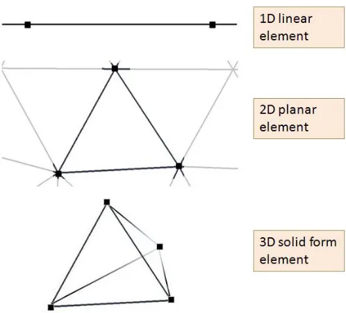
Figure 25 - Linear, triangular and tetrahedral elements as used in 1D, 2D and 3D FE simulations, respectively... 53

Figure 26 - Inward (left) and outward (right) radiative heat flux at a boundary. ... 57

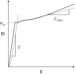
Figure 27 - Idealised stress-strain curve depicting Young’s modulus E, yield stress point σys and isotropic tangent modulus ETISO... 61

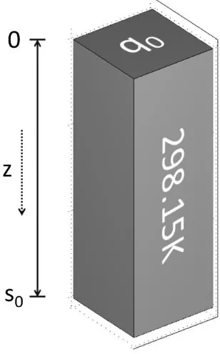
Figure 28 - Idealised depiction of geometry for the 1D heat equation. ... 63

Figure 29 - Spatial and temporal distribution of nodes used for the 1D heat equation. ... 64

Figure 30 - Idealised depiction of geometry for the 1D solution of Fick’s second law ... 67

Figure 32 - Electrox intensity distribution as obtained by 3D laser profiling of a perspex beam print (top) and 2D profile trough centre of the beam compared with an ideal Gaussian intensity distribution (bottom)... 73 Figure 33 – Schematic diagram of edge clamped cantilever arrangement with component

length (L) and sheet thickness (s0). Dashed-dot lines represent irradiation path and

direction... 74 Figure 34 -Screenshot of custom software used in edge effects investigation. ... 75 Figure 35 - COMSOL Multiphysics FE model output for the top surface directly on the laser scan line (80 x 80 x 1.5 mm mild steel AISI 1010, 760 W, 5.5 mm beam diameter, 35 mm/s, 80% absorption, edge clamped). ... 76 Figure 36 - Experimentally determined stress-strain curve for AISI 1010 mild steel... 77 Figure 37 - Experimental and theoretical elastic portion of the stress strain curve (AISI 1010).

... 77 Figure 38 - Meshed geometry used in FE simulations. ... 78 Figure 39 - 3D plot of Gaussian intensity distribution created in MATLAB... 79 Figure 40 -Screenshot from COMSOL Multiphysics illustrating how interpolation functions

can be used to apply temperature dependent material properties... 80 Figure 41 - FE simulation of temperature at 10mm and 22mm from the irradiation path over the first six passes (80 x 80 x 1.5 mm mild steel AISI 1010, 760 W, 5.5 mm beam diameter, 35 mm/s, 80% absorption). ... 82 Figure 42 - FE Experimental and simulated bend angle per pass over the first six passes (80 x 80 x 1.5 mm mild steel AISI 1010, 760 W, 5.5 mm beam diameter, 35 mm/s, 80% absorption). ... 83 Figure 43 - Effect of varying k, Cp and αth on the cumulative bend angle after six passes (80 x

80 x 1.5 mm mild steel AISI 1010, 760 W, 5.5 mm beam diameter, 35 mm/s, 80% absorption). ... 83 Figure 44 - The effect of varying Cp (top) and k (bottom) on α... 85

Figure 46 - Single pass FE simulation of volume fraction of none-ferritic phases on the top surface at the centre of the sheet (80 x 80 x 1.5 mm mild steel AISI 1010, 760 W, 5.5

mm beam diameter, 80% absorption). ... 88

Figure 47 - Single pass FE simulation of temporal cooling rate on the top surface at the centre of the sheet for a) 35 mm/s and b) 17.5 mm/s (80 x 80 x 1.5 mm mild steel AISI 1010, 760 W, 5.5 mm beam diameter, 80% absorption). ... 89

Figure 48 - Simulated martensite volume fraction on the surface of the substrate at the leaving edge after a single irradiation. (80 x 80 x 1.5 mm mild steel AISI 1010, 760 W, 5.5 mm beam diameter, 35 mm/s, 80% absorption)... 90

Figure 49 - Cumulative bend angle (80 x 80 x 1.5 mm mild steel AISI 1010, 760 W, 5.5 mm beam diameter, 35 mm/s, force cooled)... 91

Figure 50 - Microscope image of heat affected zone (80 x 80 x 1.5 mm mild steel AISI 1010, 760 W, 5.5 mm beam diameter, 35 mm/s, 1 scan, 200x). ... 92

Figure 51 - Vickers hardness variation with increasing z-depth along irradiation path (80 x 80 x 1.5 mm mild steel AISI 1010, 760 W, 5.5 mm beam diameter, 35 mm/s, 60 scans). 93 Figure 52 - Cumulative bend angle and the bend angle per pass for a) experimental and b) simulation of LF (80 x 80 x 1.5 mm mild steel AISI 1010, 760 W, 5.5 mm beam diameter, 35 mm/s, 80% absorption). ... 94

Figure 53 - Cumulative bend angle (80 x 80 x 1.5 mm mild steel AISI 1010, 760 W, 5.5 mm beam diameter, 35 mm/s, force cooled)... 95

Figure 54 - The geometrical effect in LF for an edge clamped arrangement. ... 96

Figure 55 - Effect of reducing energy density on simulated initial bend angle (80 x 80 x 1.5 mm mild steel AISI 1010, 760 W, 5.5 mm beam diameter, 35 mm/s, 80% absorption). ... 97

Figure 56 - Single pass FE simulation of edge effects with different scan strategies (80 x 80 x 1.5 mm mild steel AISI 1010, 760 W, 5.5 mm beam diameter, 80% absorption). ... 98

Figure 57 - Edge clamped rotation stage arrangement... 100

Figure 58 - Faro Arm 3D profiling system. ... 101

Figure 59 - Screenshot of the IP_Draw GUI. ... 102

Figure 60 - Screenshot of the Jog Controller and terminal. ... 103

Figure 62 - Meshed geometry used in FE simulations. ... 104 Figure 63 - Experimental (top) and simulated (bottom) initial bend angle in degrees as a

function of traverse speed, power and distance from focus. ... 105 Figure 64 - Two geometries used in the FE simulations. ... 106 Figure 65 - FE simulated z-displacement in metres for two geometries using TGM process

parameters (mild steel AISI 1010, 800 W, 6 mm beam diameter, 50 mm/s, 80% absorption). ... 107 Figure 66 - Depiction of in-plane shortening of component. ... 108 Figure 67 – Scan strategy A. Dashed-dot lines represent irradiation path and direction. ... 109 Figure 68 - Simulated x, y and z displacement (500 W, 8 mm beam diameter, 10 mm/s, 80% absorption). ... 110 Figure 69 – FE simulated z and x-displacement in metres, top and bottom respectively (mild steel AISI 1010, 500 W, 8 mm beam diameter, 10 mm/s, 80% absorption, 20x deformation scale factor). ... 111 Figure 70 - Scan strategy B. Dashed-dot lines represent irradiation path and direction. ... 112 Figure 71 - Simulated x, y and z displacement (500 W, 8 mm beam diameter, 10 mm/s, 80% absorption). ... 112 Figure 72 - Experimental scan strategy B. Dashed-dot lines represent irradiation path and

direction... 113 Figure 73 - 3D profile of a) formed component, b) side on view revealing significant

z-displacement, c) close up of side on view and d) top down view revealing minimal x-displacement... 114 Figure 74 – Appearance of HAZ after ten iterations of scan strategy B at powers of (a) 300 W, (b) 400 W and (c) 500 W (8 mm beam diameter, 10 mm/s). ... 115 Figure 75 - Bend angle after ten iterations of scan strategy B at various powers (8 mm beam diameter, 10 mm/s traverse speed)... 115 Figure 76 - Cumulative bend angle for multiple iterations of scan strategy B (400 W power, 8 mm beam diameter, 10 mm/s traverse speed)... 116 Figure 77 – Schematic diagram depicting (a) scan strategy C and (b) irradiation path for

Figure 78 - Simulated overall displacement (400 W, 8 mm beam diameter, 10 mm/s, 80% absorption, 20x deformation scale factor)... 117 Figure 79 - Simulated overall displacement at the end of the component with FE

post-processing image superimposed (400 W, 8 mm beam diameter, 10 mm/s, 80% absorption, 20x deformation scale factor)... 118 Figure 80 - Experimental scan strategy C. Dashed-dot lines represent irradiation path and

direction... 119 Figure 81 - Experimental (left) and simulated (right) total displacement at the end of the

component (400 W, 8 mm beam diameter, 10 mm/s, 80% absorption). ... 119 Figure 82 – Schematic illustration of the LμF process... 121 Figure 83 - Schematic of stainless steel AISI 302 actuator style arms, with dimensions in μm. The dashed line represents the irradiation path used in laser forming of the actuators.

... 122 Figure 84 - Number of pulses per spot and degree of pulse overlap (35 μm beam diameter, 5 kHz repetition rate, 50 mm/s traverse speed)... 123 Figure 85 - The workpiece delivery set-up on the High-Q system: 1) laser source, 2) beam expander, 3) beam steering mirrors, 4) scanning galvanometer and 5) Aerotech 3-axis stage... 123 Figure 86 - Heat diffusion depth with increasing pulse length for AISI 302 stainless steel. 125 Figure 87 - Custom designed sample holder: (a) aluminium frame, (b) ridge used for

alignment purposes and (c) Perspex grid and arrangement of actuator arms. ... 125 Figure 88 - Example output from Veeco NT1100 WLI... 126 Figure 89 - Screenshot the Alpha_B MATLAB GUI. ... 127 Figure 90 - Schematic of truncated stainless steel AISI 302 actuator style arms geometry used in FE simulations. ... 127 Figure 91 - Meshed geometry used in the FE simulations. ... 128 Figure 92 - Screenshot of the Pulse Shape Generator MATLAB GUI. 1) Laser process

Figure 93 - Time steps taken by solver during pulsed laser simulation (500 kHz repetition rate)... 131 Figure 94 - D2 against Ep (top) and D2 against Φ0, plotted on a Log10 scale (bottom)... 133

Figure 95 - Simulated temperature at the centre of the irradiation path and at four powers (1000 x 300 x 50 μm stainless steel AISI 302, 1500 mW, 35 μm beam diameter, continuous wave, 35 mm/s traverse speed)... 134 Figure 96 – FE simulated temperature (K) after a single irradiation of the geometry (1000 x 300 x 50 μm stainless steel AISI 302, 1500mW, 35 μm beam diameter, continuous wave, 10 mm/s traverse speed)... 135 Figure 97 - WLI image showing deformation of an actuator arm after 10 irradiations (1000 x 300 x 50μm stainless steel AISI 302, 0.02 W average power, 30 μm beam diameter, 1 kHz repetition rate, 10 mm/s traverse speed)... 136 Figure 98 - Profile view of z-deformation after 10 irradiations at 200 and 500 kHz repetition rate and 3μJ pulse energy (1000 x 300 x 50 μm stainless steel AISI 302, 35 μm beam diameter, 10 mm/s traverse speed)... 137 Figure 99 - FE simulation of temperature directly beneath the beam for a stationary laser heat source at 200 kHz and 500 kHz (1000 x 300 x 50 μm stainless steel AISI 302, 3 μJ pulse energy, 35 μm beam diameter). ... 137 Figure 100 - Cumulative bend angle variation with successive irradiations (1000 x 300 x 50

ACKNOWLEDGMENTS

First of all, I would like to thank my supervisors Professor Ken Watkins and Dr Geoff Dearden for their help and support throughout my PhD and assistance in the preparation of this manuscript. In addition, special thanks go to Dr Stuart Edwardson for guidance throughout the course of this investigation and without whose expertise in the field of laser forming this work would not have been possible.

I would also like to thank all the members of the Laser Group at the University of Liverpool over the last 4 years; Leigh Mellor, Joe Croft, Olivier Allegre, Kenneth Edwards, Craig Williams, Walter Perrie, Jian Cheng, Dun Liu, Zheng Kuang, Dan Wellburn, Taku Sato and Eamonn Fearon. Thanks also to Andy Snaylam, Dave Atkinson and Tony Topping for their endless assistance in setting up experiments, using equipment and preparing samples, as without them this work could not have been conducted. I would also like to thank all postgraduate students I’ve worked with over the course of my PhD for contributions made to it, especially Thomas Boegelien.

I would especially like to thank MATLAB ‘gurus’ Marco Prandina and Yazdi Harmin for their invaluable assistance, as well as for the much welcome coffee breaks at 10.30 am, 3 pm, and 5.30 pm (not to mention 11 am at weekends). I would also like to thank Denise Bain for her advice and guidance over the years.

I would like to thank Juan Jacobo ‘Jay Jay’ Angulo, Nick ‘John Gooseman’ Underwood, Samuel Bautista Lazo, Elizabeth Christie, David ‘Spanish Dave’ Vallespin, Simao Marques, Sean Malkeson, Savio Varghese, Cathy Johnson, Stephen Lawson and Marina Carrion for their superb friendship and for keeping me entertained at lunch over the years. Special thanks go to Paul ‘Fitzy’ Fitzsimons for sorting absolutely everything out in the flat, being a fantastic colleague and an even better friend.

NOMENCLATURE

A3 – Upper critical transformation temperature (K)

Cp - Specific heat capacity (J/kg.K)

C0 – Initial carbon concentration (%wt)

Cs – Carbon concentration on surface (%wt)

d0 – Beam diameter (m)

D0 – Proportionality constant (m2/s)

D – Diffusion coefficient (m2/s) E - Young’s modulus (Pa) Ep – Pulse energy (J)

ETISO - Isotropic tangent modulus (Pa)

f – Volume fraction (1) F0 – Fourier number

G – Net inward radiation (W/m2) H – Enthalpy (J)

h - Heat transfer coefficient (W/m2K) J – Radiosity (W/m2)

k - Thermal conductivity (W/m.K) l – Heat diffusion length (m)

Ms – Martensite start temperature (K)

Mf – Martensite finish temperature (K)

P - Power (W) p – Pressure (bar)

p0 – Initial pressure (bar)

Q – Activation energy of diffusion (J/mol) q0 – Boundary heat source (W/m2)

q – Net flux of radiation (W/m2) R - Universal gas constant (J/mol/K) s0 – Sheet thickness (m)

Tamb – Ambient temperature (K)

Tinf – reference temperature (K)

U – Overall heat transfer co-efficient (W/m2) v0 - Traverse speed (m/s)

Vm – Volume fraction of martensite (1)

Greek symbols

α - Thermal diffusivity (1/K)

αB – Bend angle (Deg)

αfe – Ferrite

αth - Thermal expansion co-efficient (1/K)

ε0 – Initial strain (1)

εth – Thermal strain (1)

εel – Elastic strain (1)

εp – Plastic strain (1)

ε – Total strain (1)

λ – Wavelength (m)

ν - Poisson’s ratio (1)

ρ - Density (kg/m3)

σ - Stress (Pa)

σs – Stefan Boltzmann constant (J/mol/K)

σys - Yield strength (Pa)

Φ – Fluence (J/m2)

Φth – Ablation threshold fluence (J/m2)

GLOSSARY OF TERMS

BM – Buckling mechanism CCD – Charge coupled device CCR – Critical cooling rate CR – Cooling rate

CW – Continuous wave FE – Finite element FD – Finite difference HAZ - Heat affected zone LBA – Laser beam analysis LF – Laser forming

LμF – Laser micro-forming LSH – Laser surface hardening LSμF – Laser shock micro-forming

MEMS – Microelectromechanical systems PDE – Partial differential equation

SEM – Scanning electron microscope TEM – Transverse electromagnetic mode TGM – Temperature gradient mechanism

Introduction

The work presented in this thesis focuses on the use of both numerical simulation and analytical models to gain a better understanding of the mechanism of the laser forming (LF) process at macro and micro scales.

At the macro scale, LF [1,2] is a process for the shaping or correction of distortion in metallic components through the application of laser radiation, without the need for permanent dies or tools. The non-contact nature of the process has the advantage of no tool-wear, as well as sharing the high degree of flexibility associated with other laser based process such as cutting [3-5] and marking [6,7].

The process typically involves the use of defocused infrared laser radiation to thermally induce stresses in components. Through manipulation of process parameters [8] and depending on workpiece geometry, either localized plastic compressive strains or elastic-plastic buckling can be achieved, producing out of plane bends in either direction (that is, towards or away from the beam) or in-plane shrinkage.

At the micro scale, MEMS manufacturing requires accurate positioning of components as well as a high degree of reproducibility [9]. Laser micro forming (LμF) can be utilized in accurate post-fabrication adjustment of such components, allowing for manufacturing processes with relatively large tolerances [10]. The non-contact nature of the process is also useful in accessing specific micro-components within a device which may be highly sensitive to mechanical force. As such it has potential for widespread application in both the manufacturing and microelectronics industry.

known as laser shock hardening) [13]. Utilizing shockwaves generated through the breakdown of an absorptive layer, the LSμF process induces compressive stresses in the materials upper surface, typically using nanosecond pulsed laser systems [14-16]. High repetition rate femtosecond pulsed systems have also been applied to the LSμF process, producing bending away from the beam when used in conjunction with a pre-bend induced by favourable clamping conditions [17,18].

Whilst firmly established as a process in a research environment, both LF and LμF have had limited application in industry thus far due to an inadequate understanding of aspects of the process, leading to insufficient process control. In order for laser forming to realize its potential as a fully controlled process in a manufacturing environment, an increased understanding of the complex interrelation between processing parameters [19] and the influence of component geometry is essential.

Numerical modelling can be used to simulate the LF process prior to experimentation, thereby determining the suitability of the process for the shaping of specific components. In addition, process parameter optimization can be conducted numerically, significantly reducing process development time and cost.

Such an approach requires the development of a robust and non-case specific model of the LF process, which is capable of accurately predicting both the nature and magnitude of deformation for a given combination of processing parameters and component geometry. A key additional consideration is the effect of laser processing on the subsequent performance properties of the component as a result of potential metallurgical transformations.

Research Objectives

The primary objective of this thesis is to develop a robust numerical simulation of the LF process for steels, capable of predicting the nature and magnitude of deformation for a given combination of processing parameters and component geometry. The model will subsequently be applied to the following:

per pass after multiple irradiations. Thermal-mechanical FE simulations will be used to ascertain which of the various factors (such as absorptive coating degradation, geometrical effects, variation in absorption, etc.) identified contributes towards this phenomenon and subsequently the magnitude of their contribution.

ƒ A numerical study into the process suitability and subsequent optimization of processing parameters for the LF of square section, mild steel tubes for the automotive industry.

ƒ An experimental and numerical investigation into the mechanism of deformation upon the application of short and ultra-short pulse durations in the thermal LμF of actuator-style components.

Thesis Structure

This thesis is structured as follows:

Chapter 1 provides a background on the laser heating process and how, through control of process parameters, the nature of laser induced thermal cycles can yield three distinct LF mechanisms. A summary of the metallurgical characteristics of steels during laser heating is also presented.

A review of the state of the art in both numerical modelling of the LF process at macro scales and a summary of the recent developments in LF at micro scales is presented in Chapters 2 and 3 respectively.

In Chapter 5, the various analytical and numerical models developed in Chapter 4 are applied in an investigation into the controlling factors in LF, with specific consideration given to the fall off in bend angle per pass which is evident in multiple pass LF.

Chapter 6 presents a feasibility study into the laser forming of square section mild steel tubes for the automotive industry. The suitability of the LF process is assessed and process parameter regimes identified through use of the models detailed in Chapter 4. These models were also applied to the development of suitable scan strategies for the axial bending and in-plane twisting of the components, with analogous experimentation conducted for validation purposes.

Chapter 7 presents a numerical and experimental investigation into an entirely novel mechanism for LμF of micro-scale components (<1000 μm in their largest dimension), with empirical results being used to examine and optimize laser processing parameters for process development purposes.

Chapter 1

LITERATURE REVIEW

Laser forming involves the use of thermally induced stresses to plastically deform a component, typically a metallic substrate. Through control of process parameters and depending on workpiece geometry, either localised plastic compressive strains or elastic-plastic buckling can be achieved [1].

The process has its origins in flame bending, a process in which an oxy-acetylene torch is employed as a heat source [20-22]. Whilst suitable for the forming of large, thick section components, such as the constituent parts of a ships hull, the relatively crude nature of the heat source means that flame bending has reached the limits of applicability in the shaping of smaller, more geometrically complex components. Lasers offer increased selectivity in terms of heating and a higher degree of controllability, with far greater potential for process automation.

This chapter details the theoretical background of the laser heating process, with specific emphasis on how the nature of laser induced thermal cycles can yield three distinct LF mechanisms through control of process parameters such as laser power, speed and spot size. In addition, a summary of the metallurgical characteristics of steels during laser heating is presented.

1.1 The Laser Heating Process

Laser heating of a substrate is generally the most important factor in laser based processes. In the simplest case, this will result in heating with no loss of mass and cooling due primarily to conduction away from the irradiated area. At higher powers and intensities, however, phase change and material ejection may occur. Therefore, models of laser heating must take into consideration conductive, convective and radiative heat transfer. The stages of the laser heating process are illustrated in Figure 1.

Figure 1 – Stages of the laser heating process with (a) solid heating, (b) melting, (c) liquid heating and (d) vaporization where Lf and Lv

are the latent heats of fusion and vaporization respectively.

The laser beam acts as a circular heat source on the surface with a heat flux distribution determined by the beam intensity distribution or transverse electromagnetic mode (TEM). The rate of heating observed is often dependant on the absorptivity of the metal surface relative to the wavelength of the laser radiation. As a rule of thumb, highly reflective surfaces (such as aluminium) typically require the use of shorter wavelength beams in order to ensure sufficient coupling of laser radiation into the surface of the material [29].

In the case of pulsed lasers typically applied at micro-scales, pulse duration times are generally lower than the thermal response time of the substrate, thus a steady state is never achieved. This limits heating to within a thin layer on the substrate surface. Conversely, continuous wave (CW) lasers used primarily in macro-scale applications result in conduction limited heating of the substrate, with the lateral and axial heat flux governed by the thermal properties of the substrate.

If the intensity of the beam and the irradiation time are sufficient, solid state phase transformations may occur, altering the microstructure of the substrate. Thermal properties which are of key importance in the LF process (see Section 1.2) such as thermal conductivity, density and thermal expansion coefficient are affected by the crystal structure of the metal lattice [30]. As such, the temperature dependence of material properties is a key consideration in modelling of the laser heating process. Upon further heating a thin layer on the substrate surface can become molten. This introduces solid to liquid phase change into what previously would have been a simple heat transfer process. Such phase transformations are associated with variation in energy per unit mass (enthalpy) with temperature according to the laws of thermodynamics.

Mass removal now takes place due to the surface liquid boiling away, accompanied by vapour ejection. The shear force of the reaction on the liquid surface also typically has the effect of pushing the liquid out sideways away from the beam path due the relatively lower surface tension at the hot centre of the melt pool [29].

Mathematical modelling of laser heating phenomena can provide a powerful tool for furthering an experimentalists understanding and subsequently control of a process. For instance, the results obtained from analytical models or numerical simulation can be used to predict likely outcomes or improve the efficiency of a process without the need for lengthy experimentation [31-33].

Providing the combination of process parameters used is suitable, LF is a sub-melting laser heating process. The atomic vibrations resulting from Fresnel absorption manifest themselves in thermal expansion, which can lead to elastic or plastic deformation. The localized nature of laser heating ensures that thermal expansion is restricted by the cold bulk of the substrate, often leading to compressive forces acting on the irradiated area causing plastic deformation. The following section details how, through control of process parameters and component geometry, three distinct forming mechanisms of forming can be achieved.

1.2 Laser Forming Mechanism Overview

Figure 2 - Desired heating isotherms throughout the workpiece thickness for the three principle LF mechanisms. The arrows depict the bend direction for edge clamped components.

The following subsections discuss each mechanism in detail.

1.2.1 Temperature gradient mechanism (TGM)

The mechanism most commonly employed in this work is the temperature gradient mechanism (TGM), which bends the sheet metal out of plane towards the beam. A steep thermal gradient is generated locally along the irradiation path, causing the softer upper material to plastically deform. Upon cooling, providing the temperature was raised enough to cause sufficient thermal strain, elastic contraction of the previously plastically deformed material occurs on this upper surface, yielding a bend angle of 1 to 2o _{per pass. The temporal}

Figure 3 - Simulated displacement at the edge of the sheet as a function of processing time in the TGM (80 x 80 x 1.5 mm mild steel AISI 1010, 760 W, 5.5 mm beam diameter, 35 mm/s traverse speed, 80% absorption).

In order to establish the required thermal gradient the depth of heating must be relatively small compared to the sheet thickness, this being achieved through a suitable combination of traverse speed, spot size and laser power.

During the initial stages of laser heating, purely elastic strains are induced within the irradiated area on the upper surface of the component. These elastic strains manifest themselves as differential thermal expansion throughout the sheet thickness, causing the sheet to bend away from the beam slightly in a stage of the process known as counterbending. The magnitude of this counterbend is negligible compared to the resulting bend angle but is nevertheless detrimental to the process, as it reduces the proportion of thermal strain that is converted into plastic strain and therefore residual deformation.

Upon further heating the stress induced by thermal strain exceeds the yield strength of the material, which has decreased with increasing temperature. Further thermal expansion is restricted by the cold surrounding material, resulting in plastic deformation in the heated area. This is aided by a reduction in flow stress as a result of increased temperature.

for the most part by a process of self quenching, in which heat is transferred to the cold surrounding material by conduction. Whilst convective and radiative heat transfer to the surroundings also contribute to the cooling process, the large temperature gradient between the irradiated area and the bulk makes self quenching the predominant mechanism. Therefore, material properties such as the thermal diffusivity of the workpiece are important considerations when choosing suitable process parameters.

During cooling, shrinkage occurs in the heated material. Due to plastic compression undergone during heating, the surface layer is shorter after cooling to room temperature than the bottom layer. This difference in degree of shortening throughout the component thickness results in the sheet bending out-of plane towards the beam.

temperature and therefore a reduction in thermal strain, leaving plastic and residual elastic strain. In addition, the compressive stress reduces and becomes tensile.

Figure 4 - Typical stress-strain path during a laser scan with 0→a) initial heating and restriction of thermal expansion, a→b) increasing temperature and reduction of flow stress, b→2) compressive strain development, 2→c) residual plastic strain and 2→3) compressive stress reduction to tensile stress [36].

Whilst firmly established as the most commonly applied LF technique, the mechanism by which the TGM induces deformation is subject to debate. Pirch and Wissenbach [37] noted that, for process parameters which satisfy the conditions for the TGM (that is, the establishment of a steep thermal gradient throughout the thickness of the sheet) there exists a critical number of irradiations, after which no further deformation occurs. It was proposed that, by irradiating the bottom surface after this critical irradiation number was reached, that bend angles of up to 180o _{were possible, as demonstrated numerically. However, this is in}

LF using the TGM is typically an incremental process due to the relatively small initial bend angles obtained. Whilst the bend angle per pass is fairly constant initially (typically over the first 15 to 20 passes) there is a fall off in the angle of bending achieved with successive irradiations after this. The effect of process parameters, material properties and workpiece geometry on the variation in bend angle per pass in straight line forming of flat sheets is a focus of the experimental and numerical work detailed in Chapter 5 of this thesis.

1.2.2 Buckling mechanism (BM)

Large beam diameters relative to workpiece thicknesses coupled with low traverse speeds typically result in elastic-plastic buckling, which can cause deformation towards or away from the beam [40,41].

The process parameters ensure that, during heating, there is as small a temperature gradient throughout the thickness of the sheet as possible, resulting in near homogeneous thermal expansion in the irradiated area. This produces in-plane thermal strain (εth) in x or y on both

the top and bottom surfaces, as expressed by:

T th th =α Δ

ε (1)

where αth is the thermal expansion co-efficient and ΔT is change in temperature.

Theoretically, the value for εth on the irradiated surface should always be greater than on the

bottom surface due to the inability to establish an entirely uniform temperature gradient in LF. However, in practice an instability (or ‘buckle’) typically forms across the workpiece as a result of the near homogeneous thermal expansion in the irradiated area. The direction of this instablility can be influenced by external factors, such as plastic pre-bending or applied elastic force. In the absence of such an external factor the direction of the buckle can also be influenced by residual stresses in the substrate.

As previously stated the bend direction is dependent on residual stresses in the component or externally applied stress. Such external force could be applied in the form of a gas jet but more often takes the form of mechanical pressure or restriction.

Alternatively, a slight pre-bend in the desired direction can be employed to make the forming process by buckling more predictable. This can be achieved through mechanical force or indeed a single pass of the laser using TGM process parameters.

1.2.3 Upsetting mechanism (UM)

The UM is a mechanism of in-plane shortening in which BM process parameters are applied to a workpiece geometry that restricts out of plane bending [1].

Ideally, homogeneous heating is applied throughout the thickness of the workpiece. Thermal expansion in the irradiated area occurs as a result of this heating, reducing the flow stress of the material. As in the TGM and BM, this thermal expansion is restricted by the cold surrounding material and, providing the thermal strain induced is sufficiently high, this causes compressive stresses to develop, resulting in in-plane shortening of the workpiece. As encountered in the BM, it is not possible in practice to achieve an entirely uniform temperature throughout the thickness of the sheet. Therefore, this slight temperature gradient manifests itself as a difference in thermal expansion, and subsequently shrinkage upon cooling. Unlike in the BM, buckle formation is prevented due to a relatively larger moment of inertia in the workpiece, leading to deformation towards the beam.

This slight bend towards the beam can be reduced by tailoring the process parameters to diminish the temperature gradient induced, typically through reduction of the traverse speed of the beam. Shi et al. [42] proposed a heating method in which both the top and bottom surfaces are irradiated simultaneously, reducing the dependence of temperature gradient on traverse speed as well as the out of plane deformation observed, allowing for higher throughput times.

1.2.4 Effect of process parameters

in the LF process. The process parameters, along with geometry requirements and bend direction, for each of the three principle LF mechanisms are summarized in Table 1.

Mechanism Traverse

speed

Spot size

Power Section

thickness

Bend direction

TGM High Small High Thin Out of plane towards beam

BM Low Large Low Thin Out of plane either

direction

UM Low Large Low Thick In-plane shortening

Table 1 - LF mechanism process characteristics.

As highlighted in Table 1, laser power, traverse speed and spot size are the three main process parameters in LF when using CW laser sources. For pulsed laser sources, such as those commonly used in micro-scale laser forming (see Chapter 3), pulse duration and repetition rate also play an important role.

Whilst the information in Table 1 is useful as a general rule, it is important to quantitatively establish which mechanism dominates for a given combination process parameters and workpiece geometry. The Fourier number, Equation (2), is a useful quantitative indication of the likely mechanism [43]:

2 0 0

0 0

s v

d

F ₌αth ₍₂₎

where d0 is the beam diameter, v0 is the traverse speed and s0 is the sheet thickness. The

Fourier number can be used to characterize the nature of heat conduction for a given laser-material interaction time, equal to the beam diameter divided by the traverse speed (d0/v0).

For thin section sheets, low Fourier numbers suggest that the TGM will be the predominant mechanism, with the BM and UM operating at higher Fourier numbers. Typically, Fourier numbers of less than 1 correspond to TGM parameters [13], although much higher values have been shown to result in bending towards the beam in practice.

independently of all other process parameters. Between Fourier numbers of 6.25 and 6.6 the TGM mechanism dominated due to the steep thermal gradient induced throughout the sheet thickness, as indicated by out of plane bending towards the beam. However, for Fourier number values between 6.6 and 6.8, Li identified a critical region in which neither the TGM or BM dominated; the bend direction fluctuated between towards and away from the beam. At higher Fourier values the bend direction was always away from the beam.

The Fourier number correctly identifies laser power, traverse speed, beam diameter, and sheet thickness as key factors influencing the mechanism by which deformation in LF occurs whilst also taking into account the thermal diffusivity (αth) of the substrate. Shi et al. [45]

identified the critical conditions under which the BM is the dominant mechanism for thin sheet LF, Equation (3), taking into account the Poisson’s ratio (v) of the substrate:

th

p k v A

s v s C d s P α π

ρ 3 20.76(1 )

3 0 0 0 0 2 0 + ≥ ⎟ ⎟ ⎠ ⎞ ⎜ ⎜ ⎝ ⎛

− (3)

where P is the power, s0 is the sheet thickness, d0 is the beam diameter, v0 is the traverse

speed, k is the thermal conductivity, ρ is the density, Cp is the specific heat capacity and A is

the absorption co-efficient.

1.3 Metallurgy of Steels during Laser Forming

As mentioned in Section 2.1, the generation of heat as a result of the application of laser radiation is the most significant aspect of the majority of laser based processes. It is therefore important to be cognisant of the effect of the induced thermal cycle on the metallurgical properties of the component during processing.

Applications such as laser surface hardening (LSH) [46] use the selective nature of laser heating to induce metallurgical change in components to improve wear resistance and corrosion properties in specific areas where it is needed.

The stable forms of iron in iron-carbon alloys at room temperature are ferrite (αfe) or the

metastable intermediate compound iron-carbide, known as cementite (Fe3C). Ferrite has a

body centred cubic (BCC) crystal structure (see Figure 5). For pure iron, upon heating to above 1185 K αfe fully transforms to face centred cubic (FCC) austenite, or γ-iron. Further

heating to above 1665 K results in the austenite transforming to BCC δ-iron, before melting occurs at 1810 K.

Figure 5 – Space filling models for BCC (αfe and δ-iron) and FCC (γ

-iron) crystal structures [46].

The microstructural composition at elevated temperatures is also dictated by the carbon concentration in the alloy, the addition of which to ferritic iron has a significant strengthening effect on the material. Carbon in iron is an interstitial alloying constituent with varying degrees of solubility in the various phases. Due to the shape and size of the interstitial sites in BCC and FCC crystal structures, the maximum solubility of carbon in austenite (2.14 wt%) is approximately 100 times greater than in ferrite (0.022 wt%).

1.3.1 Kinetics of austenite formation

Whilst the iron-carbon equilibrium phase diagram describes the temperature dependence of crystal structure in steels, given the short heating times associated with the LF process, it is necessary to consider the time dependence or rate such transformations.

The ferrite to austenite (αfe→γ) transformation involves the nucleation of γ phase from the αfe

matrix and growth of the γ phase by diffusion. Austenite nucleates on ferrite grain boundaries and grows rapidly into the parent phase. This solid-state transformation behaves kinetically, with the volume fraction f of austenite as a function of time t described by the Johnson-Mehl-Avrami (JMA) equation; an equation which can be used to describe the kinetics of transformations involving nucleation and growth [47-51]. At constant temperature, the JMA equation can be expressed as:

n fe f exp (k(T)t)

1−α = = − (4)

where n the JMA time exponent, a non temperature dependant constant whose value is determined by the nucleation and growth mechanism. The equation describes three different processes that occur during the transformation; nucleation, growth and the impingement of the grains of the new phase. The term k(T) is the temperature dependant rate constant for nucleation and growth rate and can be calculated using the Arrhenius equation:

⎟⎟ ⎠ ⎞ ⎜⎜ ⎝ ⎛ −

= RTi Q

i k e

T

k( ) ₀ (5)

where Q is the activation energy of the αfe→γ transformation involving both the nucleation

1.3.2 Martensitic transformation on cooling

Martensite is a non-equilibrium phase in steels and as such does not appear on the iron-carbon equilibrium phase diagram. When cooling following austenitization in the heat treatment of steels, providing the cooling rate is sufficiently low, transformation of austenite to ferrite occurs due to the instability of austenite at room temperature.

Martensite formation occurs when austenitized iron-carbon alloys are rapidly cooled (or ‘quenched’) at high cooling rates (CR). A diffusionless shear displacement of iron atoms in the FCC austenite lattice occurs as a result of this rapid temperature change, trapping any carbon present in the interstitial sites due to insufficient time for diffusion to take place [52]. The result is a supersaturated solution of carbon in iron with a body centred tetragonal (BCT) crystal structure, similar to BCC ferrite although with one elongated (or ‘distorted’) dimension [53]. The amount of distortion is dependent on the carbon content of the structure. Martensitic transformation initiates when cooling reaches the martensite start temperature (Ms). The Ms temperature is dictated by the relative abundance of alloying elements which

can enter into solid solution in austenite, according to Equation (6).

) (% 5 . 7 ) (% 1 . 12 ) (% 7 . 17 ) (% 4 . 30 ) (% 423 539 )

( C C Mn Ni Cr Mo

M o

s = − − − − − (6)

A progressively larger volume fraction of austenite is transformed to martensite until the martensite finish (Mf) temperature is reached and the transformation is complete. At this

temperature all austenite should have transformed to martensite. However, a small volume fraction of austenite is often not transformed and is referred to as retained austenite. The volume fraction of retained austenite in quenched steels typically increases with increasing relative abundance of alloying elements as the Mf temperature is reduced, sometimes to below

room temperature.

For martensite to form, rapid cooling is required so that the metastable austenite phase reaches the Ms temperature and higher temperature transformations, such as the austenite to

diagrams for a given steel [54]. Using CCT diagrams, the final microstructural composition of steel for a given cooling rate can be predicted. Depending upon where the superimposed cooling rate intersects the curves, which represent the various phases, predicts the resulting microstructure. For only martensite to form, the superimposed cooling rate should not intersect any of the curves prior to reaching the Ms temperature. It should be noted that

martensite can co-exist with other microstructures.

Martensitic steels typically exhibit high hardness and tensile strengths. However, they are also brittle, exhibiting negligible ductility. Due to the higher density of austenite compared to martensite there is a net volume increase upon martensitic transformation in steels. This phenomena has been exploited in the LSH technique to improve the fatigue properties of components by selectively inducing martensitic transformation on the surface. The aforementioned volume expansion associated with the transformation leads to the development of compressive stresses on the surface of the component. As fatigue cracks are often initiated by surface tensile stresses, such stresses must be sufficient to overcome this residual compressive stress prior to crack formation and propagation [13]. However, during the LF process martensitic transformation is highly undesirable due to its detrimental impact on the ductility of the component. As such, the induced thermal cycle forms an important consideration when selecting appropriate process parameters in LF.

1.3.3 Diffusivity of carbon and Fick’s second law

Carbon exhibits rapid diffusivity in iron due to its relatively small size when compared to other alloying elements in steel, a phenomena that has exploited by metallurgists to increase the hardness of steels in a process called carburizing [55]. During carburization, steels are typically heated in a furnace with a carbon rich atmosphere, such as in the presence of CO, to within their austenitic range (approximately 1300 K). This results in a carbon concentration gradient in the steel, facilitating solid-state diffusion of carbon into the surface. Upon appropriate heat treatment, such high carbon surfaces can be made to exhibit greater strength and wear resistance relative to the bulk of the component.

is selectively melted in the presence of a carbon source such as graphite. Laser carburizing can also proceed by solid-state diffusion of carbon into austenite in the steel surface. This is of particular relevance to the laser forming process because, as detailed in Section 4.2.3, absorptive coatings are often required as a means of increasing the coupling efficiency of laser radiation into the substrate. The coating most commonly used is graphite in the form of a spray, due to the ease at which it can be removed after processing and the high coupling efficiencies that can be achieved (approximately 80% for wavelengths of 10.6 μm). During laser heating carbon from this absorptive coating can diffuse into the component surface, thereby increasing the hardness. As such, the thermal cycle induced by the laser on the surface of the component is an important consideration regarding solid-state diffusion of carbon during the LF process. The relationship between time at elevated temperature t and carbon concentration at depth z is given by Fick’s 2nd law of diffusion [58]:

2 2 z C D t C ∂ ∂ = ∂ ∂ (7)

where C is the concentration of carbon and D is the temperature dependent diffusion co-efficient (m2/s) which can be calculated using:

⎟ ⎠ ⎞ ⎜ ⎝ ⎛ − = RT Q e D

D ₀ (8)

where D0 is the proportionality constant (m2/s), Q is the activation energy of diffusion

(J/mol), T is the temperature (K) and R is the universal gas constant (8.3 J/mol/K) where D0

Chapter 2

STATE OF THE ART IN MODELLING OF LASER

FORMING

Extensive work has been conducted on modelling the LF process. Initially, analytical models were developed, the aim of which was to assess the suitability of various combinations of process parameters and give a reasonable estimate of the bend angle. With the increasing processing power of computers, ever more accurate numerical models of the LF process have been developed which have allowed the user to assess the applicability of process parameters and scan strategies in conjunction with complex, realistic geometries.

Shen [59] summarized the development of LF modelling since its origins in the 1980s, as shown in Figure 6.

Figure 6 - Development of LF modelling [59].

experiments in an iterative heuristic approach. However, for the purposes of this investigation the focus will be on explicit simulation of the process.

The following subsections detail the state of the art in both analytical and numerical modelling of the LF process relevant to this thesis.

2.1 Analytical Modelling

Vollertsen [62] proposed an analytical or ‘trivial’ model of the TGM in which a slice through the section of a substrate is considered. This section comprises two layers; an upper layer heated by laser and a bottom layer, which remains at room temperature. Firstly, the temperature gradient (ΔT) is calculated using:

p C s lv AP T 0 0 2 ρ =

Δ (9)

where A is the absorption co-efficient, P is the laser power, ρ is the density, v0 is the traverse

speed, s0 is the sheet thickness, l is the initial length of the heated zone and Cp is the specific

heat capacity. The heat flux is then used to calculate the change in length (Δl) as a result of linear thermal expansion per unit length in the heated layer:

p th th C s v AP Tl l 0 0 2 ρ α

α Δ =

=

Δ (10)

where αth is the coefficient of thermal expansion. Assuming that all thermal expansion results

in plastic compression this can then be translated into a net bending angle (αB) for small

angles from entirely geometrical considerations (11).

0 2 2 tan s l B B _{⎟≈ =} Δ

⎠ ⎞ ⎜ ⎝

⎛α α

(11)

Therefore, the solution for the bend angle (αB) in the TGM according to the two-layer model

p th B

C s v

AP s

l

2 0 0 0

4 2

ρ α

α = Δ = (12)

The two-layer model is depicted in Figure 7.

Figure 7 – Graphical illustration of the trivial model [62].

A number of assumptions are made in the trivial model, the most striking of which are the step profile of the temperature distribution throughout the thickness of the sheet and the non-dependence of the net bending angle on the forces and moments during cooling of the sheet. Additionally, all linear expansion results in plastic deformation, which would not be the case in reality. As a result of the latter, the bend angle is typically over-estimated.

modulus (E) and yield strength (σys) of the substrate were considered. The equation for the net

bend angle according to Yau’s model is:

E s l s v C PA l ys p th B 0 2 0 0 36 2 2 σ ρ α

α = − (13)

where l is the half length of the heated zone. Another solution to the overestimation of bend angle in the trivial model proposed by Liu et al. [64] simply involved the introduction of a correction factor (η) to the laser power (ηP) to account for heat losses to the surroundings and elastic deformation during counterbending.

As previously mentioned, a key assumption in the trivial model is a non-dependence of bending angle on forces and moments during cooling of the sheet. Also, the heated layer is arbitrarily considered to be half the sheet thickness, thereby not allowing for consideration of thermal conductivity. To address these assumptions, Vollertsen proposed the two-layer model; another geometrically based model for prediction of the bend angle in TGM dominated LF processes, also comprising a heated and non-heated layer [35].

Figure 8 - Graphical illustration of the two-layer model [63].

In this model, the bend angle is defined geometrically by the difference in strains between a heated upper layer (ε1) and non-heated lower (ε2) layer according to Equation (14).

0 1 2 5 . 0 ) ( 2 2 tan s l B

B α ε ε

α − = ≈ ⎟ ⎠ ⎞ ⎜ ⎝

The normal strain in the upper and lower layers can be calculated using Equations (15) and (16) respectively: T z I E M A E F thΔ + − = α ε ₁ 1 1 1 1 1

1 (15)

2 2 2 2 2 2 2 z I E M A E F ₋ =

ε (16)

where F is the bending force, E is the Young’s modulus, A is the section area, M is the bending moment and I is the second moment of area. There is no thermal expansion term in Equation (16) as it is assumed that the lower layer remains un-heated. A further assumption is that all thermal expansion results in plastic deformation, as was the case for the trivial model. Therefore, on cooling the strain in the upper layer is given by Equation (17).

T z I E M A E F thΔ − − = α ε ₁ 1 1 1 1 1

1 (17)

By combining Equations (16) and (17) for the local strains of the top and bottom layers an expression for the net bending angle can be derived, Equation (18).

3 0

1 0 1( )

12 s s s Tls th B − Δ = α

α (18)

This expression, however, contains three unknown parameters; the temperature gradient (ΔT), length of the heated layer (l1) and thickness of the heated layer (s1). As shown in Equation

(9), the temperature rise in the heated layer is dependent upon the sheet thickness and length of the heated layer. Thus, by using an energy approach, these parameters can be calculated simultaneously. It is arbitrarily assumed that the thickness of the heated layer is half the sheet thickness. This allows for the formulation of an expression for bending angle using only known parameters, Equation (19).

p th B C s v AP 2 0 0 3 ρ α

More recently, Shen [65] developed a model which utilized an analytical solution to the heat equation (see Section 4.2.1 for more detail on the heat equation) to calculate more realistic temperature gradients throughout the sheet thickness:

∑

0 ( , ) [ ( , ) ( , )]

) , (

n

n n T t z z t T z t T T z t

T (20)

where z is the distance from the irradiated surface and n is the current time step number. The model proceeds in a iterative fashion, with the results for the temperature gradient throughout the thickness of the substrate being used to calculate the corresponding stress and strain, as related by: UL PL EL E E E E E E TISO ys TISO ys ys ⎪ ⎪ ⎪ ⎩ ⎪ ⎪ ⎪ ⎨ ⎧ ⎟⎟ ⎠ ⎞ ⎜⎜ ⎝ ⎛ − − + − + = 1 1 ) (σ_max σ σ

σ σ σ

σ

ε_σ (21)

where ETISO is the tangent modulus of plastic deformation and σmax is the maximum stress in

the loading history. EL, PL and UL refer to elastic loading, plastic loading and unloading, with the latter also applicable to reloading. It should be noted that this model neglects work hardening and creep effects. Both the Young’s modulus and plastic deformation modulus are temperature dependent and defined by a bi-linear approximation of a stress/strain curve (see Section 4.1.2.2).

A key advantage of Shens model is its ability to predict the mechanism of deformation for a given combination of process parameters, as the characteristic depth of plastic compression is predicted. The model showed good agreement with existing experimental data for single pass LF for both TGM and BM process parameter regimes.

Figure 9 - Schematic diagram of angular deformation in the heated region with sheet thickness (h) and bend angle (αB) [66].

During laser heating, differential thermal expansion as a result of a steep laser induced thermal gradient results in non uniform thermal expansion. Due to the constraint of thermal expansion in zone 1 as a result of the unheated zones either side of it, the total thermal expansion (ΔLT) consists of both plastic and elastic components:

E P

T L L

L =Δ +Δ

Δ (22)

where ΔLE and ΔLP are the elastic and plastic deformations respectively. The elastic

deformation can be expressed as follows:

) ( ) ( T E T d

L_E = eσys

Δ (23)

Where σys is the yield strength, de is the width of the deformation zone and E is the Young’s

modulus. Due to the difficulty in implementing temperature dependent material properties in analytical models, the ratio of yield strength to Young’s modulus over a temperature range of 20 to 600 oC was averaged to 1.727x10-3. From Figure 9, the bend angle can be determined geometrically on the basis of differential thermal expansion:

h L L r R L

L_{P P P P}

B 1 2 1 2

Δ − Δ = − Δ − Δ =