Modelling catastrophe risk bonds

(1)

Modelling Catastrophe Risk Bonds

Thesis submitted in accordance with the requirements of

the University of Liverpool for the degree of Doctor in Philosophy

in Mathematical Science

by

Jia Shao

(2)

Abstract

Insurance companies are seeking more adequate liquidity funds to cover the insured property losses related to nature and man-made disasters. Past experience shows that the losses caused by catastrophic events, such as earthquakes, tsunamis, floods or hur-ricanes, are extremely large. One of the alternative methods of covering these extreme losses is to transfer part of the risk to the financial markets, by issuing catastrophe-linked bonds.

This thesis focuses on model and value Catastrophe (CAT) risk bonds. The find-ings of this thesis is twofold. First, we study the pricing process for CAT bonds with different model setups. Second, based on different framework, we structured three catastrophe based (earthquake, general and nuclear risk) bonds, estimated the param-eters of the model by employing real world data and obtained numerical results using Monte Carlo simulation. Comparison between different models is also conducted.

(3)

Publications

• Shao, J., Pantelous, A., and Papaioannou, A.(2015). Catastrophe Risk Bonds With Applications To Earthquakes.European Actuarial Journal,5(1), pages113 –138.

• Ayyub, B. M., Pantelous, A., and Shao, J.(2015). Towards Resilience to Catas-trophic Events: Financing Liabilities via Catastrophe Risk Bonds.Economics of Community Disaster Resilience (NIST-ASCE) Workshop: Background

Informa-tion and Technical Papers, pages94 – 105.

• Ayyub, B. M., Pantelous, A., and Shao, J.(2015). Towards Resilience to Nu-clear Accidents: Financing NuNu-clear Liabilities via Catastrophe Risk Bonds. Un-der review since May 2015, ASCE-ASME Journal of Risk and Uncertainty in Engineering Systems, Part B: Mechanical Engineering.

(7)

List of Figures

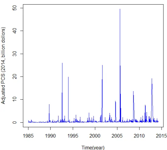
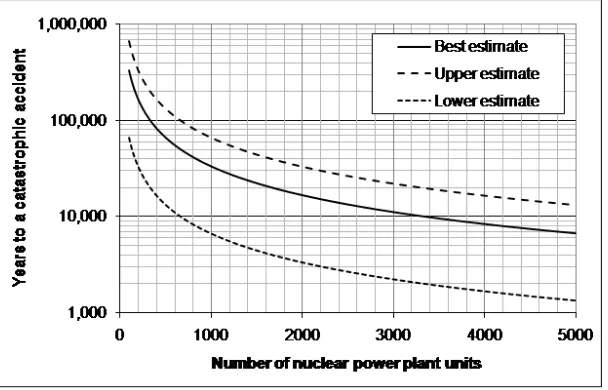
1.1 Annual catastrophe loss in the USA in 1985–2013, data from PCS. . . 3 1.2 Time to a catastrophic nuclear accident as a function of the number of

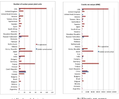
nuclear power plant units worldwide, Griffith et al. (1990). . . 4 1.3 Nuclear power plant units worldwide, in operation and under

construc-tion, as of March 10, 2015, European Nuclear Society (2015). . . 5 1.4 Global stock of debt and equity outstanding, US$Trillion, end of

pe-riod, constant 2011 exchange rates, Lund et al. (2013). . . 10 1.5 Structure of CAT bonds. . . 12 1.6 Catastrophe bonds & ILS outstanding by coupon pricing, data from

Artemis, accessed on 01/07/2015. . . 13 1.7 Catastrophe bonds & ILS outstanding by trigger type, data from Artemis,

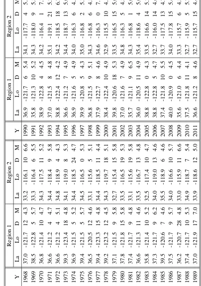
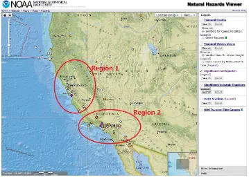
accessed on 01/07/2015. . . 14 3.1 Recent significant earthquakes in California with highlighted regions,

source by NOAA. . . 46 3.2 Scatter plot of the annual maximum-magnitude earthquakesM1(t)in

region1andM2₍_t₎_{in region}₂_{in California, 1968 – 2011. . . .} ₄₇

3.3 Diagnostic plots for GEV fitting to the annual maximum-magnitude earthquakesM1₍_t₎_{in region}₁_{in California. . . .} ₄₉

3.4 Sample mean excess for annual maximum-magnitude earthquakesM1(t) in region1in California, with95%confidence interval. . . 50 3.5 Density depth plot for the annual maximum-magnitude earthquakes

(8)

3.6 Density plot and cumulative density plot of the CAT bond price after running the algorithm100times withh= 100,000. . . 54 4.1 PCS annual catastrophe losses (left) and the number of catastrophes

(right) in the USA during 1985 – 2013. . . 69 4.2 Sample trajectories of the aggregate loss process in the USA during

1985–2013. . . 71 4.3 CAT bonds prices (z-coordinate axes) for the payoff function P_CAT(1)

under the GEV, the NHPP, and stochastic interest rate assumptions. The time to maturity (T) decreases on the left axes and threshold level (D) increases on the right axes. . . 74 4.4 CAT bonds prices (z-coordinate axes) for the payoff function P_CAT(2)

under the GEV, the NHPP, and stochastic interest rate assumptions. The time to maturity (T) decreases on the left axes and the threshold level (D) increases on the right axes. . . 75 4.5 CAT bonds prices (z-coordinate axes) for the payoff function P_CAT(3)

under the GEV, the NHPP, and stochastic interest rate assumptions. The time to maturity (T) decreases on the left axes and the threshold level (D) increases on the right axes. . . 75 4.6 CAT bonds prices (z-coordinate axes) for the payoff function P_CAT(4)

under the GEV, the NHPP, and stochastic interest rate assumptions. The time to maturity (T) decreases on the left axes and the threshold level (D) increases on the right axes. . . 76 4.7 Differences (z-coordinate axes) in the CAT bond prices forP_CAT(1)

un-der the GEV (or lognormal), the NHPP, and stochastic interest rate assumptions. The time to maturity (T) decreases on the left axes and the threshold level (D) increases on the right axes. . . 77 5.1 The nuclear power risks (five risks as an example) with respect to the

(9)

(10)

List of Tables

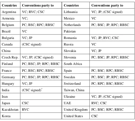
1.1 Nuclear power countries and liability conventions to which they are party, World Nuclear Association (2015). . . 8 3.1 Annual maximum-magnitude earthquakes in two regions in California,

data from SCEC. . . 45 3.2 Annual maximum-magnitude earthquakes exceeding probabilities for

the GEV model in regions1and2in California. . . 51 4.1 The 20 most costly insured CAT losses in the USA during 1985 – 2013. 70 4.2 Parameters of the semi-Markov process model. . . 72 4.3 Characteristic CAT bond prices for the payoff functionP_CAT(1) . . . 78 5.1 Vaule of N-CAT bonds with face value US$1,000for time to the

(11)

Acknowledgement

I would like to thank my supervisor Dr. Thanasi Pantelous for his tremendous support and encouragement throughout my PhD study. This thesis could not be completed without his original ideas. Thank you for training me to grow as a research scientist. Your advices on both research as well as on my career have been invaluable.

My thanks also goes to Dr. Apostolos Papaioannou for his supervision and sug-gestions on my research. Many thanks to all the staffs and students in Institute for Financial and Actuarial Mathematics (IFAM), thank you for providing such a lovely environment for me to learn and grow. Special thanks to my two examiners: Prof. Athanasios Yannacopoulos and Dr. Bujar Gashi for their kindly help and advice, which make the whole exam process so smoothly.

Thanks the GTA funding programme from the department which make it possible for me to live and learn in Liverpool.

(12)

Chapter 1 Introduction

Due to the potentially enormous financial demands on insurance (reinsurance) busi-nesses and the increasing difficulty of covering catastrophic losses by reinsurance, it is considerable to introduce a securitization method to protect vulnerable individuals. In-surance companies alleviate part of their risks by introducing securitization mechanics to achieve a more adequate liquidity fund. An alternative method is to issue catastrophe (CAT) bonds, which transfer the financial consequences of catastrophic events from is-suers to investors in a contract to cover huge liabilities through traditional reinsurance providers or governmental budgets.

CAT bonds spread the risks to another level – global financial markets. Investors take on a specific set of risks (generally catastrophe and natural disaster risks) of a specified catastrophe or event occurring in return for attractive rates of investment. If a predetermined catastrophe or event occurs, the investors will lose the principal they invested and the issuer (often insurance or reinsurance companies) will receive that money to cover their losses.

The aim of this thesis is to model and value the price of the catastrophe risk bonds. Our structure of catastrophe risk bonds involve different catastrophic perils (earth-quake and nuclear power risk) with different payoff functions and interest rate models. This thesis gives a dynamic view of modelling CAT bonds, and finally numerically computes and then compares between the prices under the different scenarios.

(13)

presents the definition of catastrophe and catastrophic risks. It also answers the ques-tion of what is the size of loss of a catastrophic event and what is the probability of having a catastrophic event occur in the given period. Section 1.2 illustrates the cur-rent nuclear liability conventions and also the liability limitation regimes. Section 1.3 provides the definition and structure of CAT bonds and then introduces the CAT bonds history. And finally in Section 1.4 is the literature review of pricing CAT bonds.

1.1 Catastrophic Events and Catastrophic Risks

A catastrophic event is defined to be a sudden event that causes one person or a group of people to suffer, or that makes difficulties. Catastrophic accidents include earthquakes, nuclear and chemical accidents, extreme storms, super-volcanoes, outer space related events, pandemics, etc. Such events occur infrequently, but cause massive losses over a short period. The Insurance Service Office’s (ISO’s) Property Claim Service (PCS)1 declared 254 catastrophes (in United States) that incurred damages of approximately US$112 billion between 1990 and 1996, while the losses due to Hurricane Andrew in 1992 reached US$26 billion2_{. Thus, even a single event can led to the insolvency of}

insurance companies.

Some arguments state that due to catastrophic accidents rarely occurring, an insur-ance company may not face such an event during its life time. Take nuclear accident risks as an example, a report to the United States Congress from the Presidential Com-mission on Catastrophic Nuclear Accidents in 1990, see Griffith et al. (1990), provides an estimate of a catastrophic nuclear accident probability in the United States of about 1 in a billion year per nuclear power plant (NPP) unit, i.e. a reactor. Expressing this 1_{ISO’s Property Claim Service unit is the internationally recognized authority on insured property}

losses due to catastrophes in the USA, Puerto Rico, and the US Virgin Islands. It contains information

on all the historical catastrophes since 1949, including the states affected, perils, and associated loss

estimates. http://www.verisk.com/property-claim-services/.

2_{An illustration of the PCS catastrophe loss data converted to 2014 dollars using the Consumer Prices}

Index (CPI) in US is given in Figure 1.1, e.g. the Northridge earthquake (1994) with losses of US$20

billion, 9/11 Terrorist Attacks (2001) with losses of US$25 billion, Hurricane Katrina (2005) with losses

(14)

[image:14.612.176.451.104.351.2]

Figure 1.1: Annual catastrophe loss in the USA in 1985–2013, data from PCS.

best estimate in this manner implicitly assumes no enhancements to the safety of nu-clear plants in the 1 billion years which is unrealistic.

(15)

[image:15.612.170.474.164.359.2]

(2012b) and recent Probabilistic Risk Analysis (PRA) of NPPs. Considering the un-certainties associated with underlying random variables, parameters and assumptions, the best estimate of 1 in 0.33 million can be expressed as a range of 1 in 1.66 million to 1 in 0.066 million.

Figure 1.2: Time to a catastrophic nuclear accident as a function of the number of nuclear power plant units worldwide, Griffith et al. (1990).

In light of the 2011 Fukushima disaster, recent discussion has focused on maxi-mizing the oversight power of global institutions and strengthening safety measures. Without accounting for the variation in nuclear technology, regulatory regimes, op-erators’ experience and NPP units’ ages, the worldwide probability of a catastrophic nuclear accident can be estimated as significantly greater than, by orders of magnitude, the levels provided by Griffith et al. (1990). The Fukushima and Chernobyl disasters of 2011 and 1986, respectively, provide empirical evidence for such levels. With a nuclear renaissance underway, the worldwide inventory of NPP units is expected to in-crease from 439 to 508, with corresponding inin-creases in net electric outputs as shown in Figure 1.3, European Nuclear Society (2015).

Assessing the adequacy of liability coverage requires examining the consequences of historic and postulated nuclear accidents. Most notable nuclear accidents3 in the civil power sector include: the 1979 Three Mile Island in which the containment

(16)

[image:16.612.124.512.68.392.2]

(a) Number of plant units (b) Electric net output

Figure 1.3: Nuclear power plant units worldwide, in operation and under construction, as of March 10, 2015, European Nuclear Society (2015).

(17)

1.2 Nuclear Liability Conventions and Liability

Limi-tation Regimes

Most countries with commercial nuclear programs adhere to one of the international conventions and concurrently have their own legislative regimes for nuclear liability, see Balachandran (2010); American Nuclear Insurers (2013). The national regimes implement the conventions’ principles and impose the financial security requirements that vary from country to country. The thirty-four countries that possess NPPs can be grouped as follows:

1. The first group includes those countries that are parties to one or more of the conventions, and which have their own legislative regimes. Prominent examples are France, Germany, Spain and the United Kingdom, all of which are parties to the Paris Convention (PC) and Revised Paris Protocol (RPC, not yet in force). Since 1988, parties to the Joint Protocol (JP) are treated as if they are parties to both the Vienna Convention (VC) and the PC. Seventeen countries have signed the Convention on Supplementary Compensation for Nuclear Damage (CSC), including Czech Republic, Canada, Ukraine and India, but most have not yet ratified it. In 2014 Japan and UAE passed legislation to ratify the CSC.

2. The second group includes those countries that are not parties to the conventions, but which have their own legislative regimes. Prominent examples are USA, Canada, Japan and Republic of Korea (South Korea). These countries impose strict liability on their nuclear installation operators. So they conform with the channeling requirements of the Paris and Vienna Conventions, despite not being parties to those conventions.

(18)

elements of the international nuclear liability conventions, e.g. channeling of absolute nuclear liability to the plant operator and exclusive court jurisdiction. Other countries in this group include Pakistan, with 3 NPPs. Pakistan is neither members of any international convention nor have any national legislation. Table 1.1 provides a summary of the convention and membership by country, World Nuclear Association (2015).

In addition, the US enacted a nuclear liability regime – the Price Anderson Act – to manage the risk of a nuclear accident in 1957. It has created a favorable climate for the nuclear American industry and provides US$13.6 billion in cover without cost to the public or government and without fault needing to be proven. The Act was amended over the years. Someone could arguably demonstrate that the US government is pro-viding subsidies since the coverage is far less than the potential loss, see Balachandran (2010); GAO (2004); World Nuclear Association (2015).

So far in this section, we have presented exposures from the perspectives of the public, operators and government; however, what does all this mean for a designer, builder or supplier? If the products or services are provided to a nuclear installation in a country subject to the PC or VC, the supplier likely does not need nuclear liability insurance. The supplier should not be held liable for damages resulting from a nuclear incident. Liability should be channeled to the facility operator.

(19)

[image:19.612.114.569.119.529.2]

Table 1.1: Nuclear power countries and liability conventions to which they are party, World Nuclear Association (2015).

Countries Conventions party to Countries Conventions party to

Argentina VC; RVC; CSC Lithuania VC; JP; (CSC signed)

Armenia VC; Mexico VC

Belgium PC; BSC; RPC; RBSC Netherlands PC; BSC; JP; RPC; RBSC

Brazil VC Pakistan

Bulgaria VC; JP Romania VC; JP; RVC; CSC

Canada (CSC signed) Russia VC

China Slovakia VC; JP

Czech Rep. VC; JP; (CSC signed) Slovenia PC; BSC; JP; RPC; RBSC

Finland PC; BSC; JP; RPC; RBSC South Africa

France PC; BSC; RPC; RBSC Spain PC; BSC; RPC; RBSC

Germany PC; BSC; JP; RPC; RBSC Sweden PC; BSC; JP; RPC; RBSC

Hungary VC; JP Switzerland PC; RPC; BSC; RBSC

India (CSC signed)* _{Taiwan, China}

Iran Ukraine VC; JP; (CSC signed)

Japan CSC UAE RVC; CSC

Kazakhstan RVC United Kingdom PC; BSC; RPC; RBSC

Korea United States CSC

PC = Paris Convention (PC).

RPC = 2004 Revised Paris Protocol. Not yet in force.

BSC = Brussels Supplementary Convention.

RBSC = 2004 Revised Brussels Supplementary Convention. Not yet in force.

VC = Vienna Convention.

RVC = Revised Vienna Convention.

JP = 1988 Joint Protocol.

CSC = Convention on Supplementary Compensation for Nuclear Damage (CSC), in force from 15 April 2015.

(20)

several countries for various reasons, most notably the United States, Canada, China, India and Russia.

1.3 Catastrophe Risk Bonds

Losses and recovery costs from catastrophic accidents are typically covered by a com-bination of utility companies, special insurance programs and/or governments. For example losses from the 2011 Fukushima disaster were covered primarily by the gov-ernment of Japan. Resources for this purpose are often inadequate and require a cash reserve that could be challenging to maintain. Low penetration rates for insurance leaves individuals, companies and governments to shoulder the financial losses aris-ing from catastrophic events. In emergaris-ing markets with nonexistent or immature legal regimes, liability could lead to international tensions and potentially wars, particularly in cases of cross-border exposures.

According to the information in Section 1.1, using a nuclear accident rate of10−6

per year, assuming 500 policies, loss per accident of US$5trillion, and price of a pol-icy for the break-even point can be computed to be US$10,000 per year. Obviously, an insurance model of this type would not sustain itself and would bankrupt upon the occurrence of the first catastrophic accident within the life of the present NNPs pop-ulation. Insurers covering other catastrophic perils – earthquake risk – may also face problems. According to historical information from the National Earthquake Infor-mation Center (NEIC), 12,000–14,000 earthquakes are recorded annually throughout the world4_{. In California, two or three earthquakes of magnitude}₅_.₅_{and higher occur}

annually, and these are large enough to cause moderate damage5_{. Although infrequent,}

earthquakes and their side effects, including landslides, surface fault ruptures, lique-faction, aftershock fires, and tsunamis, have huge potential to cause injury, loss of life, and property damage. The California Geological Survey6 _{has reported that more than}

4_{Accessed on 01/07/2015,} _{http://earthquake.usgs.gov/earthquakes/?source=}

sitenav.

5_{http://www.conservation.ca.gov/index/earthquakes/Pages/qh_}

earthquakes.aspx, accessed on 01/07/2015.

(21)

70% of California residents live within an area where significant earthquakes could occur in the next 50 years, according to slip rates in geological time. Therefore, the potential financial demands on insurance and reinsurance businesses make it realistic to introduce a mechanism for individuals against nature and man-made disasters.

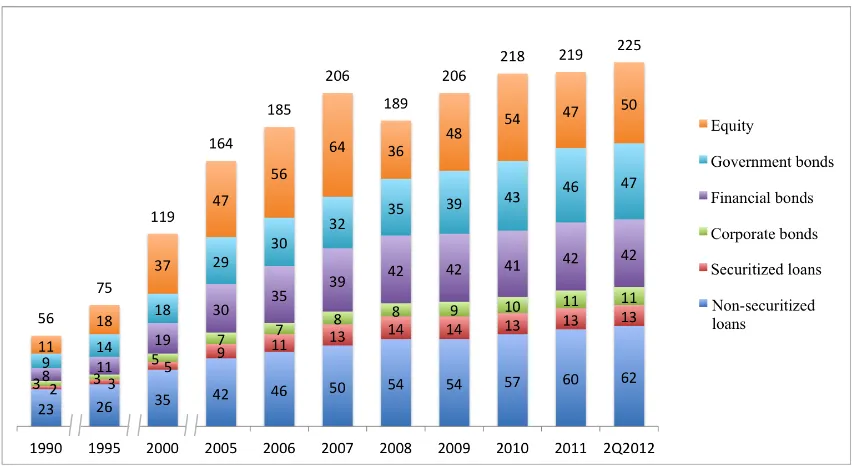
[image:21.612.114.540.332.565.2]

The requirement to achieve adequate liability coverage is to have a system that has adequate financial depth to fulfill claims. To succeed, financing is essential using special purpose instruments from the global market. Figure 1.4 provides an estimate of the 2012 global outstanding bonds and loans to be US$175Trillion out of the total US$225 Trillion of capital stock (outstanding bonds, loans and equity) with stocks at US$50 Trillion, Lund et al. (2013). Despite the 2008 financial crisis, global bonds and loan markets have increased consistently over the past twenty years from US$45 Trillion in 1990.

Figure 1.4: Global stock of debt and equity outstanding, US$Trillion, end of period, constant 2011 exchange rates, Lund et al. (2013).

(22)

finan-cial securities and their use has been accelerating in the last decade.

The first experimental transaction was completed in the mid-1990s after Hurricane Andrew and the Northridge earthquake, which incurred insurance losses of US$15.5 billion and US$12.5 billion, respectively, by a number of specialized catastrophe-oriented insurance and reinsurance companies in the USA, including AIG, Hannover Re, St Paul Re, and USAA, GAO (2002). The CAT bonds market has boomed over the years. The issued capital has increased tenfold within ten years, from less than US$0.8 billion in 1997 to over US$8billion in 2007. The issuers raised more than US$9 bil-lion of new CAT bonds in 20147. CAT bonds are inherently risky, non-indemnity-based multi-period deals, which pay a regular coupon to investors at end of each period and a final principal payment at the maturity date, if no predetermined catastrophic events occur. A major catastrophe in the secured region before the CAT bond maturity date leads to full or partial loss of the capital.

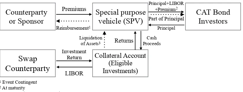
CAT bonds structure including where the capital flows from one party to another is presented in Figure 1.5. The issuer does not directly issue the CAT bond, but uses Special Purpose Vehicle (SPV) for the transaction. SPV can be interpreted as a focused insurer whose only purpose is to write one insurance contract. The existence of SPV, which is equal to a focused one-policy insurer, minimises the frictional cost of capital. Furthermore, sufficient high endowment of the SPV eliminates the counterparty risk. SPV enters into a reinsurance agreement with a sponsor or counterparty (e.g. insurer, reinsurer, or government) by issuing CAT bonds to investors and receives premiums from the sponsor in exchange for providing a pre-specified coverage. Therefore, spon-sors can transfer part of the risks to investors who bear the risk in return for higher expected returns. The SPV collects the capital (principal and premium) and invests the proceeds into a collateral account (trust account, which is typically highly related to short-term securities, e.g. Treasure bonds). The returns generated from collateral accounts are swapped for floating returns based on London Interbank Offered Rate 7_{Accessed on 17/08/2015,} _{http://www.artemis.bm/deal_directory/cat_bonds_}

ils_issued_outstanding.html. ARTEMIS is an online website since 1999, Artemis provides news, analysis and data on catastrophe bonds, insurance-linked securities and alternative reinsurance

(23)

(LIBOR) in order to immunize the sponsor and the investors from interest rate risk and default risk, Cummins (2008).

The investors coupon payments are made up of SPV investment returns, plus the premiums from the sponsor. If no trigger event occurs during the term time of the CAT bond, then the collateral is liquidated at maturity date of CAT bond and investors are repaid principal plus a compensation for bearing the catastrophe risks (solid line in Figure 1.5). However, if a trigger event occurs before the maturity, the SPV will liquidate collateral required to make the payment and reimburse the counterparty ac-cording to the terms of the catastrophe bond transaction, and CAT bond investors will only receive part of the capital (dashed line in Figure 1.5).

Counterparty

or Sponsor

CAT Bond

Investors

Collateral Account (Eligible Investments) Premiums

Reimbursement1

Principal+LIBOR +Premium2

Principal

Liquidation

of Assets3 Returns

Cash Proceeds

1_{Event Contingent} 2_{At maturity}

3_{Event contingent or at maturity}

Special purpose

vehicle (SPV)

Swap

Counterparty

LIBOR Investment

Return

[image:23.612.119.539.296.456.2]

Part of Principal

Figure 1.5: Structure of CAT bonds.

Finally, the feature of correlation of the traditional stock market allows CAT bond investors to still gain in a bad economic circumstance. CAT bonds reduce barriers to entry and increase the contestability of the reinsurance market, Froot (2001).

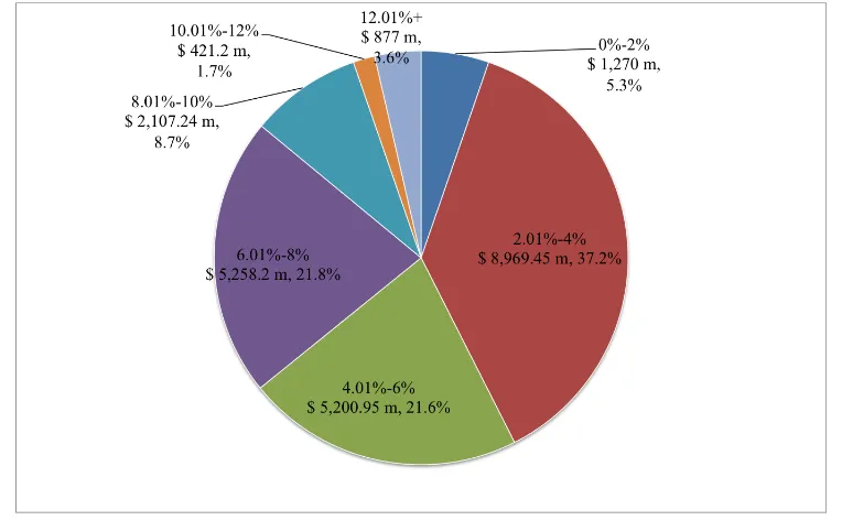
To bear the catastrophe risks, CAT bonds carry a 3 to 5 year maturity and compen-sate for a floating London Interbank Offered Rate (LIBOR) coupon plus a premium at a rate between2%and20%, see Cummins (2008); GAO (2002). Detailed information of CAT bonds premium level is given in Figure 1.68_{. One of the key elements of any}

CAT bond is the terms under which the securities begin to experience a loss. Catas-8_{Accessed on 01/07/2015,} _{http://www.artemis.bm/deal_directory/cat_bonds_}

(24)

[image:24.612.129.511.337.573.2]

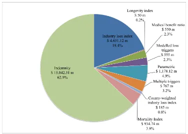
trophe bonds utilise triggers with defined parameters which have to be met to start accumulating losses. Only when these specific conditions are met do investors begin to lose their investment. Triggers can be structured in many ways from a sliding scale of actual losses experienced by the issuer (indemnity) to a trigger which is activated when industry wide losses from an event hit a certain point (industry loss trigger) to an index of weather or disaster conditions, which means actual catastrophe conditions above a certain severity will trigger a loss (parametric index trigger) etc, Hagedorn et al. (2009); Burnecki et al. (2011). Figure 1.7 presents the amount and percentage of CAT bonds issued by trigger type9. Indemnity trigger type is subject to the highest degree of moral hazard due to the fact that loss is controlled by sponsor. To tackle this problem, a better choice would be using industry loss trigger or parametric index trigger, although these might bear a relatively higher basis risk.

Figure 1.6: Catastrophe bonds & ILS outstanding by coupon pricing, data from Artemis, accessed on 01/07/2015.

CAT bonds can be structured to provide per-occurrence cover, so exposure to a single major loss event (currently US$14,850.33 million which account for 64.2%), or to provide aggregate cover, exposure to multiple events over the course of each 9_{Accessed on 01/07/2015,} _{http://www.artemis.bm/deal_directory/cat_bonds_}

(25)

[image:25.612.132.508.68.336.2]

Figure 1.7: Catastrophe bonds & ILS outstanding by trigger type, data from Artemis, accessed on 01/07/2015.

annual risk-period (US$ 8,269.14 million which account for 35.8%)10_{. Some CAT}

bonds transactions work on a multiple loss approach and so are only triggered (or portions of the deals are) by second and subsequent events. This means that sponsors can issue a deal that will only be triggered by a second landfalling hurricane to hit a certain geographical location, for example.

1.4 Literature Review

Despite the raising popularity, the number of previous studies devoted to CAT bonds pricing is relatively limited. Among the current pricing literature, authors mainly de-voted to modelling CAT bonds by different approaches, and a few have attempted to model and price from the real world perspective, in order to provide a tradeable CAT bond for a given catastrophe.

10_{Accessed on 01/07/2015,} _{http://www.artemis.bm/deal_directory/cat_bonds_}

(26)

The prediction of catastrophe risks requires an incomplete markets framework to evaluate the CAT bonds price, because the catastrophe risk cannot be replicated by a portfolio of primitive securities, see Harrison and Kreps (1979); Cox et al. (2000); Cox and Pedersen (2000); Vaugirard (2003). In the case of an incomplete market, there is no universal pricing theory that successfully addresses issues such as specification of hedging strategies and price robustness, see Young (2004). For example, Wang (2004) addressed market incompleteness using the Wang transform, an approach adopted by Lin and Cox (2005, 2008); Pelsser (2008); Galeotti et al. (2011). Froot and Posner (2000, 2002) derived an equilibrium pricing model for the uncertain parameters of multi-events risks. Follmer and Schweizer (1991) introduced a minimal martingale measure for option pricing, whereas Schweizer (1995) used a variance optimal martin-gale measure.

Another common technique used in an incomplete market setting is the principle of equivalent utility for obtaining indifferent pricing. Young (2004) calculated the price of a contingent claim under a stochastic interest rate for an exponential utility function. An extension was proposed by Egami and Young (2008), who introduced a more com-plex payment structure based on the assumption of utility indifference. Dieckmann (2011) applied a CAT bond model based on consumption, while Zhu (2011) detailed the premium spread using an intertemporal equilibrium framework. Braun (2012) anal-ysed the premium using OLS regression with robust standard errors. Cox and Pedersen (2000) used a time-repeatable representative agent utility. Their approach was based on a model of the term structure of interest rates and a probability structure for catas-trophe risks, which assumed that the agent uses a utility function to make choices about consumption streams. They applied their theoretical results to Morgan Stanley, Winterthur, USAA, and Winterthur-style bonds. Reshetar (2008) used a similar setting for multiple-event CAT bonds for the first time. Zimbidis et al. (2007) adopted the Cox and Pedersen (2000) framework to price a Greek bond using equilibrium pricing theory with dynamic interest rates.

(27)

Barysh-nikov et al. (2001) presented a continuous time no-arbitrage price of zero coupon and non-zero coupon CAT bonds that incorporated a compound doubly stochastic Poisson process. The main weakness of this paper is the authors assumed that the arbitrage measure and real world measures coincide. Burnecki and Kukla (2003) corrected and then applied their results with PCS data to calculate the arbitrage-free price of zero-coupon and zero-coupon CAT bonds. Burnecki et al. (2011) illustrated the value of CAT bonds with loss data provided by PCS when the flow of events was an inhomogeneous Poisson process. These approaches were utilized by H¨ardle and Cabrera (2010) for cal-ibrating CAT bonds prices for Mexican earthquakes. Jarrow (2010) obtained a simple closed form CAT bond solution with a LIBOR term structure of interest rate.

Another approach in continuous time is to model the trigger involving aggregate loss process. It is important to note that Vaugirard (2003) was the first to develop a simple arbitrage approach for evaluating catastrophe risk insurance-linked securi-ties, although they employed a non-traded underlying framework. In this paper, CAT bondholders have a short position on an option. Lin et al. (2008) applied a Markov-modulated Poisson process for catastrophe occurrences using a similar approach to that of Vaugirard (2003). Lee and Yu (2002, 2007) also introduced the default risk, moral hazard, and basis risk with stochastic interest rate. P´erez-Fructuoso (2008) developed a CAT bond with index triggers. Ma and Ma (2013) proposed a mixed approximation method to simplify the distribution of aggregate loss and to find the numerical solu-tions of CAT bonds with general pricing formulae. In addition, Nowak and Romaniuk (2013) expanded Vaugirard’s model and obtained CAT bond prices using Monte Carlo simulations with different payoff functions and spot interest rates.

(28)

Chapter 3 develops a model with multiple catastrophes and financial risks frame-work in a discrete-time period as an extension of the approach of Cox and Pedersen (2000). It applies an incomplete and no-arbitrage framework and assumes that all risks are mutually independent, while aggregate consumptions depend only on financial risk variables. Then, we apply theoretical results to construct a structured parametric index earthquake multi-variable CAT bond for one-period and multi-period. As a numeri-cal example, a CAT bond with historinumeri-cal data from California is proposed in which the magnitude, latitude, longitude, and depth are included in the model. In addition, appropriate models are constructed for the term structure of interest and inflation rate dynamics, and a stochastic process for the coupon rate. Finally, on the basis of analy-sis for the aforementioned catastrophe and financial market risks, we use equilibrium pricing theory to find a certain value price for the CAT California earthquake bond.

Chapter 4 derives CAT bond pricing formulae under the special case of the previ-ous chapter, one financial and one catastrophic risk. We make three main contributions to the area of CAT bond pricing. First, we construct our model in a Markov-dependent environment as an extension of the approach proposed by Ma and Ma (2013). For the first time in the CAT bonds area, we model the dependency between the claims sizes and the claim inter-arrival times for the aggregate claims as a semi-Markov process. The main benefit of this extension is the development of a more realistic model, where the occurrence time before the next claim is partially dependent on the previous claim size, which indicates that a major catastrophic event triggers many other catastrophic events in a short period. Second, in order to obtain a more complete example, we struc-ture four different payoff functions (classical zero-coupon and coupon, multi-threshold zero-coupon, and defaultable) and we give analytical formulae for CAT bonds. Third, we apply our theoretical results to construct a CAT bond and we then use PCS data to estimate relevant parameters to obtain analytical solutions, thereby providing clear guidance for practitioners.

(29)

(30)

Chapter 2 Preliminaries

2.1 Incomplete Market

Brigo and Mercurio (2007) defined in Definition 2.1.3.: ‘A financial market is complete if and only if every contingent claim is attainable.’ Harrison and Kreps (1979); Harri-son and Pliska (1981, 1983) stated the following two fundamental arbitrage-free theo-rem: Firstly, if a market exists an equivalent martingale measure (risk-neutral probabil-ity measure), then the market is arbitrage free. Secondly, if this risk-neutral probabilprobabil-ity measure is unique, then the financial market is complete. However, an arbitrage-free market does not necessarily need to be complete. In a complete market, the derivation of a unique price equals the discounted expected value of the future payoff under the risk-neutral measure. In an incomplete market, the derivative price is not unique due to the fact that one can construct several different hedging portfolios. Therefore, in order to evaluate derivatives under an incomplete framework, one can choice a suitable risk-neutral probability measure and then take the conditional expectation under this measure.

(31)

the same setting as in Section 4 of Cox and Pedersen (2000): a single period model with two tradeable zero-coupon bonds (a one-period bond and a two-period bond), when interest rate (6%) will go ‘up’ (7%) or ‘down’(5%) during this period with equal probabilities. Denote n1 as the number of one-period bonds and n2 as two -period

bonds in this portfolio, with cost 1 1.06n1+

1 1.060.5(

1 1.07 +

1

1.05)n2. (2.1)

Then, the value of the portfolio at time 1 is equal to the cash flow at time 1:

  cu cd  =  

1 ₁_.1₀₇ 1 ₁_.1₀₅

    n1 n2 

. (2.2)

Then, solve this equation to obtain:

  n1 n2  =  

1 ₁_.1₀₇ 1 ₁_.1₀₅





−1  cu cd  =  

53.5cu ₋₅₂_.₅_cd

−56.175cu+ 56.175cd



.

Substituting into Eq. (2.1) and price of cash flow[cu, cd]T at time 1 is equal to 1

1.06(0.5c

u_{+ 0}_.₅_cd_{) = 0}_.₄₇₁₇_cu_{+ 0}_.₄₇₁₇_cd_,

and this means that the model is complete. Assuming that there is additional catas-trophic risks with the condition that occurrence of catascatas-trophic event is independent of the financial variables. Therefore, the cash flows at time 1 is:

       

cu,+ cu,−

cd,+ cd,−

        .

(32)

2.2 Classical Probabilisitic Structure and Valuation

The-ory

We price CAT bonds under the following assumptions: (i) an arbitrage-free investment market exists with equivalent martingale measure, (ii) the financial market behaves independently of the occurrence of catastrophes, and (iii) the interest rate changes can be replicated using existing financial instruments.

In this section, the probabilistic structure and valuation theory for the classical model is given. We will use this structure in Chapters 4 and 5 and extend to multi-dimension in Chapter 3. Let 0 < T < ∞ be the maturity date of the continuous time trading interval[0, T]. The market uncertainty is defined on a filtered probability space(Ω,F,(Ft)t∈[0,T],P), whereFt is an increasing family ofσ-algebras, which is

given by Ft = F

(1)

t × F

(2)

t ⊂ F, for t ∈ [0, T], where F

(1)

t represents the

invest-ment information (e.g. past security prices and interest rates) available to the market at time t andF_t(2) represents the catastrophic risk information (e.g. insured property losses). The financial risk variables and the catastrophic risk variables can be mod-elled on(Ω(1)_,_F(1)_,₍_F(1)

t )t∈[0,T],P(1))and(Ω(2),F(2),(Ft(2))t∈[0,T],P(2)), respectively.

Moreover, define two filtrationsA(1) _(A(1)

t = F

(1)

t × {∅,Ω2}fort ∈ [0, T]) andA(2)

(A(2)_t ={∅,Ω1} × F (2)

t fort ∈[0, T]). It is proved by Lemma 5.1 of Cox and Pedersen

(2000) that σ-algebras A(1)_t and A(2)_t are independent under the probability measure

P. Thus, anA(Tκ) measurable random variableX on(Ω,F,(Ft)t∈[0,T],P)(or anA(κ)

adapted stochastic process Y) is said to depend only on the financial risk variables (κ= 1) or catastrophic risk variables (κ= 2).

(33)

Merton (1976); Doherty (1997); Cox and Pedersen (2000); Lee and Yu (2002); Ma and Ma (2013). According to Lemma 5.2 in Cox and Pedersen (2000), under an assump-tion that the aggregate consumpassump-tion isA(1) _{adapted (assumption (ii)), for any random}

variableXthat isA(2)_T measurable, that

EQ_[_X_{] =}_EP_[_X_]_. _(2.3)

Thus, a A(2) _{adapted aggregate loss process} _{L₍_t_{) :} _t _∈ _[0_{, T}_]_} _{retains its original}

distributional characteristics after changing from the historical estimated actual prob-ability measure_Pto the risk-neutral probability measure_Q. And the σ-algebrasA(1)_T andA(2)_T are independent under the risk-neutral probability measureQ. In an

arbitrage-free market (assumption (i)) at any timet, the price of an attainable contingent claim with payoff{P(T) : T > t} can be expressed by the fundamental theorem of asset pricing in the following form,

V(t) = _EQ₍_e−RtTr(s)dsP(T)|F

t), (2.4)

see Delbaen and Schachermayer (1994).

2.3 Interest Rate Process

There are different types of interest rates, such as government and interbank rates. Zero-coupon rates can be either from government rates which are usually deduced by bonds issued by governments or from interbank rates which are exchanged deposits be-tween banks. The most important interbank rate usually considered as a reference for contracts is the LIBOR (London InterBank Offered Rate) rate, fixed daily in London. For the purpose of bond prices, all kinds of rates are available. The first stochastic in-terest rate model was proposed by Merton (1973), followed by the pioneering approach of Vasicek (1977) and some other classical models, such as Dothan (1978); Cox et al. (1985); Ho and Lee (1986); Hull and White (1990); Black et al. (1990). In this section, we provide analysis for two interest rate models11 _{(ARIMA and CIR), which will be}

used in this thesis.

11_{Nowak and Romaniuk (2013) compared the CAT bond prices under the assumption of the spot}

(34)

2.3.1 ARIMA

The Auto-Regressive Integrated Moving Average (ARIMA) is a typical form to analyse time series data in statistics and econometrics and can be denoted as ARIMA(p, d, q), where pthe number of lags of the stationarized series in the prediction equation, or formally called ‘autoregressive terms’; d is the number of nonseasonal differences a time series needs for stationarity, called ‘integrated’; and q is the number of lagged forecast errors in the equation, called ‘moving average terms’.

Special cases of ARIMA models are as follows: • random-walk (ARIMA(0,1,0)without constant),

X(t) = X(t−1) +(t);

• exponential smoothing models (ARIMA(0,1,1)without constant), X(t) =X(t−1)−(1−α)(t−1);

• first-order autoregressive models (ARIMA(1,0,0)), X(t) = C+θX(t−1) +(t);

• first-order moving average models (ARIMA(0,0,1)), X(t) = C+(t) +α(t−1);

• damped-trend linear exponential smoothing (ARIMA(1,1,1)),

X(t)−X(t−1) =C+θ(X(t−1)−X(t−2)) +(t) +α(t−1);

whereC is a constant,θ, αare parameters and(t)is a white noise process. In partic-ular, if slope coefficientθ is close to 0, then the process looks like white noise; as θ approaches 1, the model describes mean-reverting behaviour.

For the purposes of estimating the parameters and predicting by the ARIMA model, we usearimaandpredictfunctions in R.

in the pricing process which is affected by the interest rate dynamics. Readers can refer to Brigo and

(35)

2.3.2 CIR

A typical instantaneous interest rate dynamics proposed by Cox, Ingersol, and Ross (CIR model, Cox et al. (1985)) assumed a ‘square-root’ term in the diffusion coef-ficient. This model is a benchmark because it provides analytical bonds and bond options pricing. The short-rate dynamics {r(t) : t ∈ [0, T]} under the risk-neutral measure_Qcan be expressed as follows,

dr(t) = k(θ−r(t))dt+σpr(t)dW(t), (2.5) with the condition

2kθ > σ2, (2.6)

wherer(0), k, θ, andσ are positive constants. The condition Eq. (2.6) guarantees that the processr(t)remains in the positive domain and the origin is inaccessible. Assum-ing the spot interest rate under the real world measure_Pwith the form:

dr(t) = [kθ−(k+λr)r(t)]dt+σ

p

r(t)dW∗(t), (2.7) whereW∗(t) = W(t) +Rt

0

λr

√

r(s)

σ ds is a Brownian motion under the risk measure

P andλr is a positive constant12 contributing to the market price of risk. Assuming

QandPare equivalent measures, then compare Eq. (2.5) and Eq. (2.7) and we obtain

Radon-Nikodym derivative of_Qwith respect to_P: d_Q d_P _F t

= exp −1 2

Z t

0

λ2

rr(s)

σ2 ds+

Z t

0

λr

p

r(s)

σ dW

∗

(s)

!

.

The market price of risk processλ∗_r(t)is a stochastic process with the functional form λ∗_r(t) = λr

σ

p

r(t), t∈[0, T].

For detailed information about this transformation, please refer to Ma and Ma (2013); Nowak and Romaniuk (2013); Shirakawa (2002); Lee and Yu (2002); Remillard (2013).

According to Brigo and Mercurio (2007), we can price a pure-discount T-bond at timetby the following equalities:

BCIR(t, T) = A(t, T)e−B(t,T)r(t), (2.8)

12_{For the case}_λ

r = 0, dynamics Eq. (2.5) and Eq. (2.7) coincide, where risk neutral world and

(36)

where

A(t, T) =

2he(k+λr+h)(T−t)/2

2h+ (k+λr+h)(e(T−t)h−1)

2_σkθ2

, (2.9)

B(t, T) =

2(e(T−t)h−1)

2h+ (k+λr+h)(e(T−t)h−1)

, (2.10)

h=p(k+λr)2+ 2σ2. (2.11)

We complete this subsection by giving maximum likelihood estimation of the CIR model. Glasserman (2003) stated that in the CIR model, the increments of the short-rate follows a non-central chi-square distribution and the transition density of Eq. (2.5) can be written as:

r(t) = σ

2₍₁₋_e−k(t−u)₎

4k χ

2

d

4ke−k(t−u)

σ2₍₁₋_e−k(t−u)₎r(u)

, t > u,

where,

d= 4θk

σ2 andλ =

4ke−k(t−u)

σ2₍₁₋_e−k(t−u)₎r(u).

The cumulative distribution function is

P(r(t)≤y|r(u)) = Fχ2

(d,λ)

4ky σ2₍₁₋_e−k(t−u)₎

,

and the probability density function is given as

Pr(t)(y|r(u)) =cpχ2

(d,λ)(cy),

wherep_χ2

(d,λ)(·)is the density of the non-centralχ

2_{distribution, where}

c= 4k

σ2₍₁₋_e−k(t−u)₎.

Finally, one can have the log-likelihood function:

l(θ, k, σ;y) = n

X

i=2

log(c) + n

X

i=2

log(pχ2

(d,λ)(cyi|yi−1)),

wherey = r1, . . . , rn is given according to the data. We use numerical optimization

to find the maximum likelihood estimation of the parameters and the R-function of the model is given in Appendix C.2. Alternatively, one can use the R PackageSMFI5with

(37)

2.4 Extreme Value Theory

Extreme value theory deals with the stochastic of the minimum or the maximum of a very large collection of random observations from the same arbitrary distribution. The first statement of extremal limit theorem was by Fisher and Tippett (1928), and they suggested that the behaviour of the maxima can be described by only a few forms. Thereafter, Gnedenko (1943) gave convergence to a unified version type theorem – the Generalized Extreme Value distribution (GEV). Gumbel (1958) showed statistical application of theory to estimate extremes.

SupposeX1, X2, . . . are independent and identically distributed random variables

with common cumulative distribution functionF. LetMδ = max{X1, X2, . . . , Xδ}

denote the maximum of the firstδrandom variables. In theory, the exact distribution ofMδcan be derived by

P(Mδ ≤z) =P(X1 ≤z, . . . , Xδ≤z)

=_P(X1 ≤z)· · ·P(Xδ ≤z) = (F(z))δ.

However, this is not immediately helpful in practice, since the distribution functionF is not always available. There are two possible methods to solve this problem, first is the Central Limit Theorem (CLT) and second is Fisher-Tippett-Gnedenko theorem which is discussed in this section, see Fisher and Tippett (1928); Embrechts et al. (1997); Coles et al. (2001).

Theorem 2.4.1. (Fisher–Tippett–Gnedenko)

If there exist sequences of constants{σδ : σδ > 0,∀δ ∈ N} and{βδ : δ ∈ N} such that

P

Mδ−βδ

σδ

≤z

→G(z) asδ→ ∞, z ∈_R,

then

G(z)∝exp−(1 +αz)−1/α ,

whereα depends on the tail shape of the distribution. When normalized,Gis a non-degenerate distribution function and belongs to one of the following forms (γ >0):

I. (Gumbel)G(z) = exp−exp − z−β

σ when the distribution of Mδ has an

(38)

II. (Fr´echet) G(z) =     

0 z ≤β

expn− z−_σβ−γo

z > β.

when the distribution of Mδ

has a heavy tail (including polynomial decay).

III. (Weibull)G(z) =



 

 

expn− − z−_σβγo

z < β

1 z ≥β

when the distribution ofMδ

has a light tail with finite upper bound.

These can be grouped into the the single distribution calledGeneralized Extreme

Value (GEV)distribution, with c.d.f.

G(z) = exp

(

−

1 +α

z−β σ

−1/α)

, (2.12)

defined on{z : 1 +α(z−β)/σ >0}, whereβ ∈_R,σ > 0andα ∈_R.

The model has three parameters: location parameter β, scale parameter σ, and shape parameterα. The caseα = 0is interpreted as the limitα → 0and Eq.(2.12)

corresponds to the Gumbel family. For the casesα >0(α= _γ1) andα <0(α=−1

γ),

Eq.(2.12)leads to Frech´et and Weibull family distributions, respectively.

We complete this section by giving maximum likelihood estimation for GEV dis-tribution parameters(α, σ, β). AssumingM1, . . . , Mδare independent variables with

GEV distribution, then the log-likelihood for parameters(α, σ, β)(α 6= 0) is given by

l(α, σ, β) =nlogσ−(1+1 α) δ X i=1 log

1 +α

Mi−β

σ − δ X i=1

1 +α

Mi−β

σ

−1_α

, (2.13) provided that

1 +α

Mi−β

σ

>0, fori= 1, 2, . . . , δ.

There is no analytic solution for maximize Eq. (2.13), but for any given dataset the maximization is obtained straightforwardly by using standard numerical algorithms, Coles et al. (2001). In the following chapters, we use R Package fExtremes with

(39)

Chapter 3 Multi Variables CAT Bond Model

In this chapter, a model withm catastrophe risks and n financial risks in a discrete-time period is developed as an extension of the approach of Cox and Pedersen (2000). Theoretical results are applied to construct a multi-variable CAT bond, and then use California earthquakes data to derive the price density function for a 5-year structured parametric earthquake CAT bond. This chapter works under an incomplete and no-arbitrage framework, assuming that all risks (both financial and catastrophic risks) are pairwise independent.

(40)

3.1 Modeling CAT bonds

3.1.1 Model Description and Preliminaries

In this subsection, a preliminary presentation for the CAT bond structure is given. Generalizing the ideas of Cox and Pedersen (2000), a CAT bond that combines n financial market variables and m catastrophic risk variables is designed. The model set-up requires a probabilistic structure which is given as follows.

Assume that issuers are trading CAT bonds in an investment market that is arbitrage-free. The time of the catastrophe(s) is independent of the term structure(s) under the relevant probability measure. We assume that there are n financial risk variables, each modelled on a filtered probability space (Ω1,i,F(1,i),(Ft(1,i))t=0,1,..., T,P1,i) for

i= 1, 2, . . . , n. LetT <∞be the maturity time of the trading interval. LetF_t(1,i)be theσ-algebras ofΩ1,irepresenting the investment information available to the market

at timet (t = 0, 1, . . . , T), whereF(1,i) _(i _{= 1}_, ₂_{, . . . , n) are corresponding}

filtra-tions. Thus, each probability measure _P1,i is defined for all events belonging to the

F_t(1,i)σ-algebra,t ≤ T. Note that the measures _P1,ido not necessarily have the same

distributions.

Then considermcatastrophic risk variables, which are modelled on a filtered prob-ability space (Ω2,j,F(2,j),(Ft(2,i))t=0,1,..., T,P2,j), where Ft(2,j) are the σ-algebras of Ω2,jrepresenting the catastrophic risk information available at timet(t= 0, 1, . . . , T)

and _P2,j (j = 1, 2, . . . , m) are the probability measures governing the catastrophe

structure (not necessarily with the same distribution). The filtrationsF(2,j)_{are indexed}

by the same timest= 0, 1, . . . , T as previously. The sample space of the full model can be constructed, such that

Ω =

Ω1,1×Ω1,2 × · · · ×Ω1,n

×Ω2,1×Ω2,2× · · · ×Ω2,m

.

A typical event of the full model sample space is of the formω = (ω_e1,n, ωe2,m), where e

ωκ,` = (wκ,1, wκ,2, . . . , wκ,`), κ = 1, 2, ` = n, m, such that w1,i ∈ Ω1,i (i = 1, 2, . . . , n) andw2,j ∈Ω2,j(j = 1, 2, . . . , m).

(41)

independent, then the probability measure on the sample spaceΩis given by

P(ω) =

n

Y

i=1

P1,i(ω1,i)· m

Y

j=1

P2,j(ω2,j), i= 1, 2, . . . , n, j = 1, 2, . . . , m.

In addition, the natural filtration produced by theσ-algebras ofΩis denoted byF and given by

Ft=

F_t(1,1)× F_t(1,2)× · · · × F_t(1,n)×F_t(2,1)× F_t(2,2)× · · · × F_t(2,m), fort= 0, 1, . . . , T. Thus,(Ω,F,(Ft)t=0,1,..., T,P)constitutes a probability space for

the full model with all the elements defined as above. In order to define random vari-ables in the full model that depends only on either financial varivari-ables or catastrophic variables, let us introduce the increasing filtrations A(1)_t ⊂ A(1) _and _A(1,i)

t ⊂ A(1,i)

(i = 1, . . . , n), and similarlyA(2)_t ⊂ A(2) _and_A(2,j)

t ⊂ A(2,j) (j = 1, . . . , m)

gener-ated from the followingσ-algebras:

A_t(1) =F_t(1,1)× · · · × F_t(1,n)× {∅,Ω2,1, . . . ,Ω2,m},

A(1_t ,i) =F_t(1,i)× {∅,Ω2,1, . . . ,Ω2,m}, i= 1, . . . , n,

A(2)_t ={∅,Ω1,1, . . . ,Ω1,n} × F

(2,1)

t × · · · × F

(2,m)

t ,

A(2_t ,j) ={∅,Ω1,1, . . . ,Ω1,n} × F

(2,j)

t , j = 1, . . . , m,

fort= 1, . . . , T. AnA(_Tκ)measurable random variableXon(Ω,F,(Ft)t=0,1,..., T,P)

(or an A(κ) _{adapted stochastic process} _Y_{) depends on financial risk variables (κ} ₌

1) or catastrophic risk variables (κ = 2). Let financial events be α1,i ∈ A(1_T,i) and

catastrophic events beα2,j ∈ A

(2,j)

T . We need the independent notion ofA

(κ,`)

T because

we cannot refer toF_T(κ,`) as being independent under_P, since each ofF_T(κ,`) does not contain events defined on(Ω,F,(Ft)t=0,1,..., T,P).

Lemma 3.1.1. Fori= 1, . . . , nandj = 1, . . . , m, theσ-algebrasA(1_T,i)andA(2_T,j)are independent under the probability measure_P.

Proof. Fori = 1, . . . , n andj = 1, . . . , m, we have α1,i ∈ A

(1,i)

T andα2,j ∈ A

(2,j)

T .

Therefore,α1,i =A1,i×Ω2,1× · · · ×Ω2,mfor someA1,i ∈ F

(1,i)

t , andα2,j = Ω1,1×

· · · ×Ω1,n×A2,j for someA2,j ∈ F

(2,j)

t , and we have that

P

" _n \

i=1

α1,i

\ \m

j=1

α2,j

#

=_PA1,1× · · · ×A1,n×A2,1× · · · ×A2,m

(42)

= n

Y

i=1

P1,i(A1,i)· m

Y

j=1

P2,j(A2,j)

= n

Y

i=1

P1,i(A1,i) m

Y

j=1

P2,j(Ω2,j) n

Y

i=1

P1,i(Ω1,i) m

Y

j=1

P2,j(A2,j)

= n

Y

i=1

P(α1,i)· m

Y

j=1

P(α2,j).

And the result follows.

3.1.2 The Valuation Framework

In this subsection, we show how to implement valuation under the full model by choosing the equivalent measure. Similar to Cox and Pedersen (2000) and Magill and Quinzii (2002), the setting of a representative agent is adopted to price uncertain cash flow streams, as which is the benchmark financial economics technique. By this technique, we need to assume a representative utility function and an aggregate con-sumption process.

Assume aT-period economy, in which agents can make choices and consume dur-ing each period. An agent makes choices about his future consumption, represented by the stochastic process{c(t);t= 0, 1, . . . , T}. The aggregate consumption stochastic process is denoted by {C∗₍_t_);_k _{= 0}_, ₁_{, . . . , T}_{}. Both these processes are adapted}

to filtration of the full model. Only the first choice is known with certainty at time t= 0. Fori= 1,2, . . . , n, let{ri(t);t= 0, 1, . . . , T −1}be the one-period financial

market rates. Then these one-period financial market rates can be defined through the conditional expectation

n

Y

i=1

1 1 +ri(t)

= 1

u0_k(C∗₍_t₎₎E

P_u0

t+1(C

∗

(t+ 1))|Ft

, t= 0, 1, . . . , T −1, (3.1)

whereu0, u1, . . . , uT represent the utility functions, and also assume representative

agent’s utility is additively separable and differentiable. The Randon-Nikodym deriva-tive of_Qwith respect to_Pis defined in the same vein as Cox and Pedersen (2000)

d_Q d_P =

n

Y

i=1

T−1

Y

s=0

[1 +ri(s)]

u0_T(C∗(T)) u0

0(C∗(0))

(43)

Note that this new random variable is measurable with respect toFT. In addition, we

clearly need to ensure that_EPdQ

dP

= 1(Lemma 3.1.2). First, for notation simplicity, denote the one-period financial market discount rates by

B(k) =

       n Y i=1

t−1

Y

s=0

[1 +ri(s)], fort= 1, 2, . . . , T,

1, fort= 0.

Then, define the stochastic processes{ξ(t);t= 0, 1, . . . , T}and{ζ(t);t= 0, 1. . . , T} as

ξ(t) =_EP

d_Q d_P Ft

= dQ d_P _F t

andζ(t) =B(t)· u

0

t(C

∗₍_t₎₎

u0

0(C∗(0))

,

with t = 1, . . . , T and B(0) = 1, which leads to ζ(0) = 1. By Eq. (3.2) it holds thatζ(T) = dQ

dP ∈ FT.Similar to Lemma B.1 and Theorem B.1 of Cox and Pedersen (2000), we have the following lemma and theorem.

Lemma 3.1.2. The process{ζ(t);t= 0, 1, . . . , T}is a_P-martingale on the filtration

F, andζ(t) =ξ(t)fort= 0, 1, . . . , T.

Proof. First, note that the process {ζ(t);t = 0, 1, . . . , T} is F adapted, since the processesri(t)andC∗(t)areF adapted processes, as well. Furthermore,

EP[ζ(t+ 1)|Ft] =_EP

"

B(t) n

Y

i=1

[1 +ri(t)]

u0_k(C∗(t+ 1)) u0₀(C∗₍₀₎₎

Ft #

=_EP

"

ζ(t) n

Y

i=1

[1 +ri(t)]

u0_t₊₁(C∗(t+ 1)) u0_t(C∗₍_t₎₎

Ft #

=ζ(t) n

Y

i=1

[1 +ri(t)] 1 u0_t(C∗₍_t₎₎E

P

u0_t₊₁(C∗(t+ 1))

Ft

=ζ(t),

where the last equality is obtained by using Eq. (3.1). Finally, by using the fact that the process{ζ(t);k = 0, 1, . . . , T}forms a martingale, we conclude that

ζ(t) =_EP

ζ(T)|Ft

=_EPhdQ d_P

Ft

i

(44)

Remark 3.1.1. An immediate consequence of Lemma 3.1.2 is that

1 =_EPh_ζ₍₀₎i ₌

EP

h

ζ(T)i =_EPh_ξ₍_T₎i₌

EP

hd_Q

d_P

i

,

which ensures that the Radon-Nikodym derivative in Eq. (3.2) indeed defines a new probability measure.

Intuitively, the probability measure _Q(·) is equivalent to knowledge of the repre-sentative investor’s utility function and the aggregate consumption process.

Theorem 3.1.1. Under the assumptions of the representative agent pricing model, the value of a generic future cash flow process{PCAT(t);t = 1, 2, . . . , T} at time 0is

given by

V(PCAT) =EQ

T X t=1 1 Qn i=1

Qt−1

s=0[1 +ri(s)]

PCAT(t)

=_EQ

" _T X

t=1

1

B(t)PCAT(t)

#

. (3.3)

Remark 3.1.2. When in incomplete markets, there is no unique interpretation for the prices that we assign to CAT bonds unless we introduce the probability distribution of

the catastrophe risk, see Section 2.1.

Using similar arguments to those in Theorem B.2 of Cox and Pedersen (2000), the general intertemporal valuation of a future cash flow can be expressed in terms of the equivalent measure_Q(·).

Theorem 3.1.2. Under the assumptions of the representative agent pricing model, the value of a generic future cash flow process{d(t);t =k+ 1, p+ 2, . . . , T}at timek

is given by

EP

T

X

t=k+1

u0_t(C∗(t))

u0_k(C∗₍_k₎₎PCAT(t)

Fk

=_EQ

T

X

t=k+1

B(k)

B(t)PCAT(t)

Fk ,

wherek = 0, 1, . . . , T, with the convection

a

P

b

= 0fora < b, a, b∈_N.

(45)

since global economic conditions in terms of exchange and production are not strongly related to localized catastrophes, see Cox and Pedersen (2000). Assuming that the aggregate consumption process depends only on financial risk information available at timet, and that the structure at time0is known.

Lemma 3.1.3. Under the assumption thatC∗isA(1)_{adapted, for any random variable}

Xthat isA(2)_T measurable we have

EQ_[_X_{] =}_EP_[_X_]_.

In particular, for any catastrophic eventsα2,j (j = 1, 2, . . . , m) that areA

(2,j)

T

mea-surable, it holds that

Q(

m

\

j=1

(α2,j)) =P( m

\

j=1

(α2,j)) = m

Y

j=1

P2,j(A2,j), (3.4)

whereA2,j ∈ F_T(2,j).

Proof. Note that dQ

dP in Eq. (3.2) is A

(1)

T measurable, because of the fact that C

∗

and B(T)areA(1)_{adapted. Therefore, for any random variable}_X _{that is}_A(2)

T measurable

we have thatXanddQ

dP are independent underP. Together with Lemma 3.2.5 of Shreve (2004), one can prove that

EQ[X] =EP

XdQ d_P

=_EP_[_X_]

EP

d_Q d_P

=_EP_[_X_]_·_{1 =}

EP[X].

Moreover, define

X = m

Y

j=1

1α2,j =1Tm_j₌₁α2,j,

whereα2,j ∈ A(2_T,j), j = 1,2, . . . , m. Substituting into Eq. (3.4), and obtain

Q(

m

\

j=1

(α2,j)) = EQ

h

1Tm j=1α2,j

i

=_EQ_[_X_{] =}_EP_[_X_{] =}

EP

h

1Tm j=1α2,j

i

=_P( m

\

j=1

(α2,j)) =P

m

\

j=1

Ω1,1× · · · ×Ω1,m×A2,j

= m Y j=1 " _n Y i=1

P(Ω1,j)

P(A2,j)

#

= m

Y

j=1

(46)

Remark 3.1.3. Under the measure_P(·)and the assumption thatC∗ depends only on financial risk variables, we can conclude that the catastrophic eventsα2,j that depend

on thejth catastrophic risk (j = 1, . . . , m) are independent.

To implement Theorems 3.1.1 and 3.1.2, it is crucial to assume that the events are mutually independent, that is, they depend only on financial risks and only on catastrophic risks, under the measure_Q.

Lemma 3.1.4. Under the assumption thatC∗isA(1)_{adapted, the}_σ_-algebras_A(1)

T and

A(2)_T are independent under_Q.

Proof. Letα1,i ∈ A

(1,i)

T andα2,j ∈ A

(2,j)

T . Applying Lemma 3.2.5 of Shreve (2004),

then have

Q

n

\

i=1

α1,i

\

m

\

j=1

α2,j

=_EQh1Tn

i=1α1,i1Tmj=1α2,j

i

=_EP

1Tn i=1α1,i1

Tm j=1α2,j

d_Q d_P

.

Since dQ

dP in Eq. (3.2) isA

(1)

T measurable, 1Tm

i=1α1,i

d_Q

d_P and 1

Tm j=1α2,j

are independent under_P. Consequently,

EP

1Tn

i=1α1,i1Tmj=1α2,j

d_Q d_P

=_EP

1Tn i=1α1,i

d_Q d_P

EP

h

1Tm j=1α2,j

i

=_EQ

1Tn i=1α1,i

P

m

\

j=1

α2,j

=_Q n

\

i=1

α1,i

m

Y

j=1

P2,j[α2,j].

Referring back to Lemma 3.1.3, we have

EP

1Tn

i=1α1,i1Tmj=1α2,j

d_Q d_P =_Q n \ i=1

α1,i

m

Y

j=1

P2,j[α2,j]

=_Q n

\

i=1

α1,i

Q

m

\

j=1

α2,j

.

(47)

As a direct implication of Lemmas 3.1.3 and 3.1.4, the current value of cash flows Xdepending on catastrophic risks has the simple form as below. For notation simplic-ity, we denote the current value of non-defaultable zero-coupon bond maturing at time twith face amount1asP(t) =_EQh 1

B(t)

i

.

Corollary 3.1.1. The current value of anA(2)_t measurable cash flowX paid at timet

is given by

EQ

1 B(t)X

=P(t)_EP_[_X_]_.

Under the discrete time framework, we can express the valuation measure as a product measure of the probability measures_Q1 andP2,j,

Q(ω) = dQ

d_P(ω)P(ω) =B(ω;T)u

0

T(C∗(ω;T))

u0₀(C∗₍_ω_{; 0))} P(ω)

= T−1

Y

s=0

n

Y

i=1

[1 +ri(ω1,i;s)]

u0_T(C∗(˜ω1,n;T))

u0₀(C∗_(˜_ω

1,n; 0)) n

Y

i=1

P1,i(ω1,i) m

Y

j=1

P2,j(ω2,j)

=_Q1(˜ω1,n) m

Y

j=1

P2,j(ω2,j), (3.5)

where

Q1(˜ω1,n) = T−1

Y

s=0

n

Y

i=1

[1 +ri(ω1,i;s)]

u0_T(C∗(˜ω1,n;T))

u0₀(C∗_(˜_ω

1,n; 0)) n

Y

i=1

P1,i(ω1,i). (3.6)

The probability measure in Eq. (3.6) is generated in terms of the term structure of financial risks, see Pedersen (1994). It is practical to have Eq. (3.5) since the empirical probabilities of catastrophic events can be used for the probability measures_P2,j, where

j = 1, . . . , m.

Modelling catastrophe risk bonds