Concurrent Data Structures.
White Rose Research Online URL for this paper:
http://eprints.whiterose.ac.uk/90972/
Version: Accepted Version
Article:
Schellhorn, G., Derrick, J. and Wehrheim, H. (2014) A Sound and Complete Proof
Technique for Linearizability of Concurrent Data Structures. ACM Transactions on
Computational Logic, 15 (4). 31. ISSN 1529-3785
https://doi.org/10.1145/2629496
[email protected] Reuse
Unless indicated otherwise, fulltext items are protected by copyright with all rights reserved. The copyright exception in section 29 of the Copyright, Designs and Patents Act 1988 allows the making of a single copy solely for the purpose of non-commercial research or private study within the limits of fair dealing. The publisher or other rights-holder may allow further reproduction and re-use of this version - refer to the White Rose Research Online record for this item. Where records identify the publisher as the copyright holder, users can verify any specific terms of use on the publisher’s website.
Takedown
If you consider content in White Rose Research Online to be in breach of UK law, please notify us by
A Sound and Complete Proof Technique for Linearizability of
Concurrent Data Structures
GERHARD SCHELLHORN, University of Augsburg, Germany JOHN DERRICK, University of Sheffield, UK
HEIKE WEHRHEIM, University of Paderborn, Germany
Efficient implementations of data structures such as queues, stacks or hash-tables allow for concurrent access by many processes at the same time. To increase concurrency, these algorithms often completely dispose with locking, or only lock small parts of the structure.Linearizabilityis the standard correctness criterion for such a scenario — where a concurrent object is linearizable if all of its operations appear to take effect instantaneously some time between their invocation and return.
The potential concurrent access to the shared data structure tremendously increases the complexity of the verification problem, and thus current proof techniques for showing linearizability are all tailored to specific types of data structures. In previous work we have shown how simulation-based proof conditions for linearizability can be used to verify a number of subtle concurrent algorithms. In this paper, we now show that conditions based onbackwardsimulation can be used to show linearizability ofeverylinearizable algorithm, i.e., we show that our proof technique is both soundandcomplete. We exemplify our approach by a linearizability proof of a concurrent queue, introduced in Herlihy and Wing’s landmark paper on linearizability. Except for their manual proof, none of the numerous other approaches have successfully treated this queue.
Our approach is supported by a full mechanisation: both the linearizability proofs for case studies like the queue, and the proofs of soundness and completeness have been carried out with an interactive prover, which is KIV.
Categories and Subject Descriptors: D.2.4 [Software Engineering]: Software/Program Verification General Terms: Algorithms,Verification
Additional Key Words and Phrases: Z, refinement, concurrent access, linearizability, non-atomic refinement, theorem proving, KIV
ACM Reference Format:
ACM Trans. Comput. Logic V, N, Article A (January YYYY), 35 pages. DOI = 10.1145/0000000.0000000 http://doi.acm.org/10.1145/0000000.0000000
1. INTRODUCTION
The advent of multi- and many-core processors will see an increased usage of concurrent data structures. These are implementations of data structures like queues, stacks or hash-tables which allow for concurrent access by many processes at the same time. Indeed, already libraries such asjava.util.concurrentoffer a vast number of such concurrent data structures. To increase concurrency, these algorithms often completely dispose with locking,
Gerhard Schellhorn, Universit¨at Augsburg, Institut f¨ur Informatik, 86135 Augsburg, Germany, [email protected]
John Derrick, Department of Computing, University of Sheffield, Sheffield, UK, [email protected] Heike Wehrheim, Universit¨at Paderborn, Institut f¨ur Informatik, 33098 Paderborn, Germany, [email protected]
Permission to make digital or hard copies of part or all of this work for personal or classroom use is granted without fee provided that copies are not made or distributed for profit or commercial advantage and that copies show this notice on the first page or initial screen of a display along with the full citation. Copyrights for components of this work owned by others than ACM must be honored. Abstracting with credit is permitted. To copy otherwise, to republish, to post on servers, to redistribute to lists, or to use any component of this work in other works requires prior specific permission and/or a fee. Permissions may be requested from Publications Dept., ACM, Inc., 2 Penn Plaza, Suite 701, New York, NY 10121-0701 USA, fax +1 (212) 869-0481, or [email protected].
c
YYYY ACM 1529-3785/YYYY/01-ARTA $15.00
or only lock small parts of the structure. Instead of locking, fine-grained synchronization schemes based on atomic operations (e.g., Compare-And-Swap CAS or Load-Link/Store-Conditional LL/SC) are employed in order to allow for a high degree of concurrency.
Whereas correctness for their sequential counter-parts is trivial, it can be complex and subtle for these concurrent algorithms, particularly ones that exploit the potential for con-currency to the full. For example, their design inevitably leads to race conditions. In fact, the designers of such algorithms do not aim at race-free but atlinearizablealgorithms. Lin-earizability [Herlihy and Wing 1990] requires that fine-grained implementations of access operations (e.g., insertion, lookup or removal of an element) appear as though they take effect instantaneously at some point in time, thereby achieving the same effect as an atomic operation [Herlihy and Wing 1990]:
Linearizability provides the illusion that each operation applied by concurrent processes takes effect instantaneously at some point between its invocation and its response.
Since the original approach based on possibilities, a number of other approaches to prove linearizability have appeared, and a number of algorithms have been shown to be lineariz-able [Doherty et al. 2004; Colvin et al. 2005; Abrial and Cansell 2005; Hesselink 2007; Vafeiadis et al. 2006; Amit et al. 2007; Calcagno et al. 2007; Derrick et al. 2008; 2011b]. Some of the proofs of correctness are manual, whereas others are partly supported by theo-rem provers (for instance with PVS) or fully automatic. The latter, however, either require user-annotations to the algorithm or – in the case of model checkers – only prove correctness for a limited number of parallel processes.
The proof techniques vary as well, and range from using shape analysis or separation logic to rely-guarantee reasoning and simulation-based methods. The simulation-based methods show that an abstraction (or simulation or refinement) relation exists between the abstract specification of the data structure and its concurrent implementation.
Whilst great progress has been made in the state-of-the-art in this area, a number of weaknesses remain. For example, apart from our own [Derrick et al. 2008], all current approaches only argue informally that their proof technique actually implies the original linearizability criterion of [Herlihy and Wing 1990]. Rather, they have focused on providing an efficient and practically applicable proof technique. We, however, have aimed to ensure that we always have a mechanized proof of soundness of our method in addition to any individual proof of correctness for a specific algorithm.
In addition, inspecting the current approaches, one finds that a number of techniques (including our own so far) get adapted every time a new type of algorithm is treated. Every new “trick” designers build into their algorithms to increase performance (e.g., like a mutual push and pop elimination for stacks, or lazy techniques) requires an extension of the verification approach. This is the case because the verification approaches are usually kept as simple as possible to ease their application, and in particular to allow for a high degree of automatization. Still, our motivation was to present a proof technique which can be used to prove linearizability ofeverylinearizable algorithm: we have derived a proof method that issound and complete for linearizability.
The approach is again a simulation-based method, this time based onbackward
use of simulations for showing linearizability is not new; however, current refinement-based approaches (e.g., [Doherty et al. 2004; Doherty and Moir 2009; Colvin and Groves 2005]) are
based on both backward andforward simulations. Note that our completeness result does
not imply a direct method for deriving a backward simulation for an existing linearizable data structure; it just states the existence of such a simulation. This is in line with other completeness results, e.g., for data refinement or for specific proof calculi: completeness only states the existence of a proof, never a way of deriving this proof.
We nevertheless exemplify our approach to using just backward simulations by verifying the queue implementation of Herlihy and Wing [Herlihy and Wing 1990]. None of the current approaches to linearizability have treated this algorithm; and it is also not clear whether the many approaches tailored towards heap usage (like separation logic or shape analysis based techniques) can successfully verify the queue, as the complexity in the interaction between concurrent processes in the queue is not due to a shared heap. There is no heap involved at all, rather, the underlying store is an unbounded array. Along with this queue example we also show how to systematically construct the backward simulations needed in the linearizability proofs. Although the complete methodology determines the most general backward simulation to use, in practice, it is often more convenient to use a smaller relation. We do this in the queue verification, and to this end, we provide a number of guidelines for deriving backward simulations in general.
Last, but not least, to fit our desire for a provenly correct methodology, we have a complete mechanization of our approach. It is complete in the sense that we both carry out the backward simulation proofs for our examples (here, the queue) with an interactive prover (which is KIV [Reif et al. 1998]), andhave verified within KIV that the general soundness and completeness proof of our technique is correct. Proofs for the general theory as well as for the case study can be found online at [KIV 2011].
The structure of the paper is as follows. The next section introduces our running example, the Herlihy and Wing queue. We use Z to formalize the pseudo-code of the algorithm, which will subsequently be verified in KIV. In section 3 we formally define linearizability of an abstract and a concurrent data type, and define refinement and simulations between them. The proof methodology is then derived in section 4. This is achieved by augmenting the original data types with history information and using a particular type of finalization, and showing that the abstract and concurrent data type are linearizable if and only if the augmented concurrent data type is a backward simulation of the augmented abstract data type. The proof uses a particular intermediate layer in its construction, reminiscent of the definition of possibilities in [Herlihy and Wing 1990].
We return to the queue of Herlihy and Wing in section 5 to mechanically verify a proof of its linearizability using a specific backward simulation.
For algorithms with complex linearization points, such as the queue considered here, global backward simulations are needed, since by their nature such algorithms have non-local behavior. However, for many simpler case studies it has been informally argued that simpler, local proof obligations are sufficient. Section 7 sketches, how the thread-local proof obligations we defined in [Derrick et al. 2011b] can be derived from the general backward simulation.
Finally, in sections 8 and 9 we discuss related work and some conclusions. This paper is an extended version of [Schellhorn et al. 2012] in which we present the underlying theory in full detail, the most important aspects of the KIV proof and add guidelines for the derivation of backward simulations.
2. HERLIHY-WING QUEUE
Wing 1990]. We will mix the informal description with a formalization in the specification language Z [Woodcock and Davies 1996], a state-based specification formalism which al-lows the specification of data types by defining their state (variables), initial values and operations, to describe an abstract queue and its concurrent implementation. The com-plete system then consists of a number of processes, each capable of executing its queue operations on the shared data structure. The key question we are interested in is whether the concurrent implementation is correctwith respect to the abstract specification – even though the atomic steps of the concrete can be interleaved in a manner not feasible in the abstract specification.
As usual, the queue is a data structure with two operations: enqueue appends new
ele-ments to the end of the queue and dequeue removes elements from the front of the queue.
We have one enqueueand dequeue for each processp ∈P. Abstractly, we can specify the
queue as follows. The state, initialization and operations are given as schemas, consisting of variable declarations plus predicates. We assume a given type T for queue elements.
AState q: seqT
AInit AState
q=h i
AEnqp
∆AState el? :T
q′=qahel?i
ADeqp
∆AState el! :T
q=hel!iaq′
The first two schemas in the specification fix the state,AState, of the data structure queue (a sequence of elements), and its initial value (the empty list given via its initializationAInit). As usual in Z, a sequence q =ha1, . . .aniof length n (written #q =n) is a function from
the interval from 1 ton (written 1..n) to elements of T. Operatorq1aq2 concatenates two
sequences, an element is selected with q(k) for k ∈1..n. The two operations enqueue and
dequeue for all the processes are written asAEnqp andADeqp (Afor abstract specification
andpfor the process executing it). In such a specification the primed variables refer to the value of variables in the after-state. Unprimed as well as primed variables of a particular state schema are introduced into operation schemas by the ∆-notation. Input and output variables are decorated by ? and !. In general, we can model all such data structures as abstract data types ADT = (AState,AInit,(AOpp,i)p∈P,i∈I), where the setI is used for
enumerating the abstract operations. Each operationAOpp,i is defined over the state space
AState and can additionally specify inputs and outputs. Inputs are denoted here by in? and outputs byout!, with types INi andOUTi (dependent on the operationi, but not on
the processp executing it) respectively.
The queue is implemented by an arrayAR of unbounded length. All (used) slots of the
array are initialized with a special value null6∈T, signaling ’no element present’. A back pointer back into the array stores the current upper end of the array where elements are
enqueued. Dequeues operate on the lower end of the array. An enq operation thus simply
gets a local copy of back, increments back (these two steps are executed atomically) and then stores the element to be enqueued in the array. We can describe the operations in pseudo-code as follows, where we annotate each line with a line number (E1 etc):
E0 enq(lv : T)
E1 (k,back) := (back, back+1); /* increment */
E2 AR[k]:= lv; /* store */
D0 deq(): T
D1 lback := back; k:=0; lv := null D2 if k < lback goto D3 else goto D1
D3 (lv, AR[k]) := (AR[k], lv); /* swap */ D4 if lv != null then goto D6 else goto D5 D5 k := k + 1; goto D2
D6 return(lv)
Thedeqoperation proceeds in several steps: first, it gets a local copy ofback and initializes a counterk and a local variable,lv, which is used to store the dequeued element. It then walks through the array trying to find an element to be dequeued. StepsD2 andD5 in the code above constitute a loop consecutively visiting the array elements.
At every positionk visited in the loop the array contentsAR[k] is swapped with variable
lv. If the dequeue finds a proper non-empty element this way (lv 6= null), this will be returned, otherwise searching is continued. In the case where no element can be found in the entire array,deqrestarts the search. Note that if noenq operations occur,deqwill thus run forever.
As we said, the complete system consists of a number of processes, each capable of executing its queue operations on a shared data structure. For the concrete implementation therefore these two algorithms can be executed concurrently by any number of processes — where the individual steps in the operations are atomic. So, for instance, we could have a process
p executingE1 and then a process q executingD1 and (one of the branches of)D2, then
p continuing withE2, a third processr starting yet anotherdeq with stepD1 and so on. Every interleaving of steps is possible. Formally, we can model the complete system (not just for a single process) as a data type with the following state.
CState
AR: IN→T∪ {null}
back : IN
kf :P →IN
lbackf :P →IN
lvf :P →T∪ {null}
pcf :P →PC
CInit CState
∀i : IN•AR(i) =null back = 0
In addition toAR andback (explained above), the state contains local variables for every
process from P, thus we have functions from P to the domain of the local variables. In
addition, every processphas a variablepcf(p) to denote the program counter. The program counter can take values fromPC ={N,E1,E2,E3,D1,D2,D3,D4,D5,D6}, N denoting
the idle state of a process (the idle state needs to be the same state for each operation so we useN as opposed toE0 andD0 here).
To model the operations, we introduce an operation denoting the invocation of an enqueue (enq0) or dequeue (deq0) (i.e., statementsE0 andD0), then we have one operation for every line in the program (except forif-statements which are split into a true (e.g.,deq2t) and a false (deq2f) case). Each operation then corresponds to the granularity of atomicity in the concurrent implementation.
Operation names are indexed by the process executing them. Thus in total we have operationsenq0p,enq1p,enq2p,enq3p,deq0p,deq1p,deq2tp,deq2fp,deq3p,deq4tp,deq4fp,
deq5panddeq6pfor everyp∈P. Below we see a formal definition of some of the operations.
the specifications much more readable (otherwise we would have to add a lot of predicates of the form back′ =back etc.) and has no semantic consequence. Formula pcf′(p) = E1 denotes the expansionpcf′=pcf⊕ {p7→E1}that overwritespcf(p) withE1, and similarly for the other variables and functions in the schemas. The ordering of statements within the programs for the operations are ensured by the use of program counters and appropriate preconditions for operations.
enq0p
∆CState lv? :T
pcf(p) =N ∧pcf′(p) =E1
lvf′(p) =lv?
enq1p
∆CState
pcf(p) =E1∧pcf′(p) =E2
kf′(p) =back∧back′=back+ 1
deq2tp
∆CState
kf(p)<lbackf(p)
pcf(p) =D2∧pcf′(p) =D3
deq6p
∆CState el! :T
pcf(p) =D6∧pcf′(p) =N el! =lvf(p)
Formally, this defines our concrete data type CDT = (CState,CInit,(COpj)j∈J). Our
ob-jective is to show that the concrete data type is linearizable with respect to the abstract data type, i.e., all runs of the concrete data type with whatever kind of interleaving of operations of concurrent processes resemble correct queue operations. (We will formalize the definition itself later.)
To illustrate the issue we first take a look at one run to demonstrate the interplay between the operations of different processes. So imagine the following processes executing their individual concrete operations on the shared data type. Here, the steps of processes are given and (relevant parts of) the resulting state.
(1) Process 3 starts an enqueue for the elementa (E0) and executesE1:
kf(3) = 0,pcf(3) =E2,back = 1 AR= [−,−,−, . . .]
Sequence of operations so far:henq03,enq13i
(2) Process 1 starts an enqueue for the elementb and executesE1:
kf(1) = 1,pcf(1) =E2,back = 2 AR= [−,−,−, . . .]
Sequence of operations so far:henq03,enq13,enq01,enq11i
(3) Process 2 starts a dequeue and executes D0 andD1:
kf(2) = 0,pcf(2) =D2,lbackf(2) = 2,lvf(2) =null AR= [−,−,−, . . .]
Sequence of operations so far:henq03,enq13,enq01,enq11,deq02,deq12i
(4) Process 4 starts an enqueue for the elementc and executesE0,E1,E2:
kf(4) = 2,pcf(4) =E3,back = 3 AR= [−,−,c,−, . . .]
Sequence of operations (continued):h. . . ,enq04,enq14,enq24i
(5) Process 2 continues its dequeue with D2,D3,D4,D5,D2:
kf(2) = 1,pcf(2) =D3,lbackf(2) = 2,back = 3 AR= [−,−,c,−, . . .]
(6) Process 3 finishes its enqueue executingE2 andE3:
pcf(3) =N AR= [a,−,c,−, . . .]
(7) Process 4 finishes its enqueue executingE3:
pcf(4) =N AR= [a,−,c,−, . . .]
(8) Process 2 finishes the dequeue and returnsc:
pcf(2) =N,kf(2) = 2,lbackf(2) = 2,back = 3 AR= [a,−,−,−, . . .]
(9) Process 1 finishes the enqueue:
The question of correctness is as follows: does this concrete run of operations (and its visible effect on the shared data structure) in some sense correspond to a run of the abstract specification?
In fact, it does in this case, specifically the above concrete run has (for instance) the following matching run of the abstract data type:
hAEnq4(c),ADeq2(c),AEnq3(a),AEnq1(b)i
But notice that this correct abstract run is not the initially most obvious. Specifically, one would be tempted to look at the ordering of the invocations of the operations: hAEnq3,AEnq1,ADeq2,AEnq4i, or failing that, the returns (i.e., responses) of the
oper-ations: hAEnq3,AEnq4,ADeq2,AEnq1i. Neither of these is the correct abstract sequence
necessary to give the right queue: in the first case the dequeue should returna, and in the second case as well, which it however does not.
Rather, instead of the start or the end, it is the point in time where the effect of the operation on the abstract queue becomes visible to other operations (this is known as the
linearizability point, or LP) that determines the corresponding abstract order. The effect of enqueue of c becomes visible first even though it puts the element into position 2 of the array, not 0. This is because it is the first position which the dequeue observes to be
non-empty as it has already gone past position 0 with its local array index k when the
elementa is placed in position 0.
At this moment one would be tempted to exactly find the LP of each operation, e.g., it might beE2 for enqueue andD5 for dequeue. Such an approach of finding fixed linearization points in the concurrent algorithm works for some non-locking algorithms such as Treiber’s stack [Treiber 1986] or Michael and Scott’s queue [Michael and Scott 1996]. However, for other more complex algorithms the point where the effects become visible changes from run to run according to the contents of the input/output or data structure. Examples of algorithms that are like this include the lazy set algorithm [Heller et al. 2005]. However,
the behavior of the above is even more subtle — the LP in one operation depends on what
other operations have already started — i.e., depends on the whole global history. To see this note that if the dequeue has not already gone past position 1 when process 1 enqueues
b, the dequeue would returnb rather than c. Thus, it is not only the ordering of enqueue operations of different processes which determines their abstract order, but it is also the progression of dequeues (of which we can of course also have several ones).
This intricate interplay of enqueues and dequeues makes this algorithm the hardest type for which to verify linearizability. Indeed, at first glance the hopes of finding some local
proof obligations (as opposed to reasoning about global histories) would seem remote, let alone finding a complete methodology. However, this is what the following sections seek to explore. We begin with the basic definitions.
3. BACKGROUND
Our proof technique is grounded in the theory of refinement and simulations. However, before we start with the basic terminology for these, we want to formally define the notion of linearizability. In this, we essentially follow Herlihy and Wing’s formalization.
3.1. Histories and Linearizability
Linearizability is a notion of correctness relating two specifications: a sequential abstract specification and a concurrent implementation. Here, these are both given as data types consisting of state space, the initialization and a number of operations executed by some process, i.e., like in the example we have ADT = (AState,AInit,(AOpp,i)p∈P,i∈I) where
AInit ⊆AState, andAOpp,i ⊆INi×AState×AState×OUTi. The concurrent
implementa-tion is given asCDT = (CState,CInit,(COpp,j)j∈J,p∈P) whereCInit ⊆CState. We assume
of which abstract one. We will place some restrictions onabsbelow, e.g., it will be an 1-to-n
mapping between abstract and concrete. The concrete operations can be partitioned into three classes. Invoking operations (deq0p and enq0p in the example) have input of type
INabs(j). Returning operations (deq6p andenq3p) have output of typeOUTabs(j), all others
have neither input nor output, i.e., these operations are just relations over CState.
The last example already discussed the issue of finding an appropriate run of the abstract data type for every run of the concrete implementation. Here, we will make the notion of “appropriate” or “matching” abstract run more precise.
Formally, linearizability can be defined by comparing thehistoriesformed by runs of the abstract and concrete data type. Histories are finite sequences of events. Events can be invocations and returns of particular operations by particular processes from the set P.
Event ::=invhhP×I×INiii |rethhP×I ×OUTiii
History = seqEvents
Events are defined using Z notation for free data types. Typical elements of the type are
inv(p,i,in) andret(p,i,out), wherepis a process,iis an operation index, andin∈INiand
out ∈OUTi are elements of the input resp. output type ofAOpp,i. SettingI ={enq,deq},
a possible history of our queue implementation is
h=hinv(3,enq,a),inv(1,enq,b),inv(2,deq,),inv(4,enq,c),ret(3,enq,),
ret(4,enq,),ret(2,deq,c),ret(1,enq,)i
This is the history corresponding to the above run detailed in the previous section, where, for example, ret(3,enq,) denotes the return of the enqueue operation undertaken by
pro-cess 3. The return event of enqueue has no output, thus the last argument is empty. The corresponding history of the abstract queue is
hs =hinv(4,enq,c),ret(4,enq,),inv(2,deq,),ret(2,deq,c),
inv(3,enq,a),ret(3,enq,),inv(1,enq,b),ret(1,enq,)i
Of course, there is no interleaving at the abstract level, thusret(1,enq,) immediately follows
its invocationinv(1,enq,b), that is histories of the abstract specification (like this one) will always be sequential (definition coming up). These histories are in a sense an abstraction of the concrete run (with just invocations and returns), but not as abstract as the initial specification which did not even differentiate between invocation and return. We will use them to compare our abstract and concrete runs in a fashion detailed below. First, some basic definitions.
We use predicatesinv?(e) andret?(e) to check whether an evente∈Event is an invoca-tion or a return, and we letRet! be the set of return events. We lete.p∈P be the process
executing the event e and e.i ∈I the index of the abstract operation to which the event belongs.
Not all sequences of events are correct histories of a data type. Thus we need the idea of a legal (concurrent) history: a legal history consists of matching pairs of invocation and return events plus some pending invocations, where an operation has started but not yet finished1
Definition3.1 (Legal histories). Leth: seqEventbe a sequence of events. Two positions
m,n inh form amatching pair, denotedmp(m,n,h) if
0<m<n ≤#h∧inv?(h(m))∧ret?(h(m))∧h(m).p=h(n).p∧h(m).i=h(n).i∧
∀k : IN•m <k <n ⇒h(k).p6=h(m).p
1
A positionn : 1..#hin h is apending invocation, denotedpi(n,h), if
inv?(h(n))∧ ∀m•n <m ≤#h⇒h(m).p6=h(n).p
The set of all pending invokes h(n) with pi(n,h) is denoted as pi(h). h is legal, denoted
legal(h), if
∀n : 1..#h•if inv?(h(n))thenpi(n,h)∨ ∃m: 1..#h•mp(n,m,h) else ∃m : 1..#h•mp(m,n,h)
2
Both of the above given histories are legal. In the historyh we, for instance, have matching pairs 1 and 5, mp(1,5,h), and no pending invocations (all invocations are followed by a
matching return).
Later, we will formally define how to construct histories out of a data type. For the moment note that history hs as well as all other histories of the abstract data type are
sequential. This is formalized in the following predicate:
sequ(h) ==∃n •#h= 2n∧ ∀m : 1..n•mp(m+m−1,m+m)
A (complete2) sequential history is a sequence of matching pairs. For a legal history, function
complete(h) defined as
complete(hi) =hi
complete(heiah) =if pi(1,heiah)thencomplete(h)elseheiacomplete(h)
removes all pending invocations from a legal historyh. To determine, whether a concurrent history h is linearizable it is compared with abstract sequential histories, to see whether one can be found, that matches. First of all,hmight need to be extended by some (but not necessarily all) returnsh0 ∈seqRet! that match the pending invocations. This is the case
whenhcontains operations where the effect has already taken place, though they have not returned. An example for this is the operationD3 in the dequeue: once the swap occurs on a non-empty array element, the effect of the operation has taken place although it has not returned yet. This results in a historyhah0which is now compared to a sequential history
hs according to two conditions:
L1. when projected onto processes,complete(hah0) andhs have to be equivalent, and
L2. the ordering of operation executions inhneeds to be preserved in hs.
Here, two operations are orderedif the second one starts after the first one has returned. We rephrase this in a more formal way using a bijection f (denoted →using Z notation)
betweenh andhs so that it can be used in our theorem prover:
Definition3.2 (Linearizable histories). Given two histories h,hs, we define h to be in
lin-relation withhs, denotedlin(h,hs), if ∃ f : 1..#h→1..#hs•
legal(h)∧sequ(hs)∧ ∀n : 1..#h•h(n) =hs(f(n))
∧ ∀m,n: 1..#h•mp(m,n,h)⇒f(n) =f(m) + 1
∧ ∀m,n,m′,n′: 1..#h•mp(m,n,h)∧n <m′∧mp(m′,n′,h)⇒f(n)<f(m′)
A (concrete) historyhislinearizablewith respect to some sequential (abstract) historyhs, denoted linearizable(h,hs), if
∃h0: seqRet!•legal(hah0)∧lin(complete(hah0),hs)
2
A concrete data type CDT is linearizable with respect to an abstract data type ADT if
every history ofCDT is linearizable with respect to some history ofADT. 2
Example 1:The historyh from our running example is linearizable with respect tohs. 2
Example 2:An example of a non-linearizable concrete history is
h1=hinv(1,enq,a),ret(1,enq,),inv(2,enq,b),inv(3,deq,),ret(3,deq,b)i
For it to be linearizable we would have to find a sequential history hs1 which keeps the
ordering of operations (condition L2), i.e., in which the enqueue of a comes before the
other two operations, and in which the dequeue still returns ab(condition L1). Neither the placement of the enqueue ofb before nor after the dequeue would give us a valid abstract
history. 2
3.2. Data refinement and simulations
The central aim of work on linearizability is to derive proof methods to verify that a particu-lar concurrent algorithm is linearizable. As we have seen, linearizability is a global condition defined over histories, so we are particularly interested in proof obligations that are local
(in some sense, e.g., in terms of verifying conditions on an operation per operation basis) as opposed to global so that we can avoid reasoning over all histories.
Indeed, in our previous work on proving linearizability [Derrick et al. 2008; 2011a] we have derived proof obligations that examine one step at a time instead of full runs, using the ideas ofdata refinementbetween the two data types, specifically the obligations are all based on the idea of showingsimulationsbetween the data types. That is, we have exploited the fact that simulations are step-local obligations that can verify the global refinement property. The essence of our proof method is thus to derive local proof obligations such that local
proof obligations betweenADT andCDT implyCDT to be a certain sort of refinement of
ADT which in turn can be shown to implyCDT is linearizable wrtADT.
Using these methods we have been able to verify some of the standard benchmark algo-rithms for work in this area. For example, in [Derrick et al. 2008] we show how to verify a lock-free implementation of a stack. However, the proof obligations were not complete, that is not every case of linearizability could be verified using the methodology, and to cover more complex or subtle algorithms, the proof obligations had to be adapted to tackle all new aspects. For example, the lazy set implementation [Heller et al. 2005] tackled in [Vafeiadis et al. 2006] and [Colvin et al. 2006] has linearization points set by processes other than the one executing the operation, and we needed to use more general simulation conditions to treat this aspect.
For all of our proof obligations we have a mechanized proof of soundness, i.e., we have formally shown that the validity of the proof obligations implies linearizability. Here, we are now also interested incompletenessof proof obligations: we aim to derive a proof tech-nique which is general enough to show linearizability for everylinearizable data type and algorithm. Of course, soundness needs to be kept.
The technique which we develop next is based on the idea of data refinement and simula-tions as was the original method. Essentially, we show that given an abstract and a concrete
data typeADT andCDT (representing an abstract view and concurrent implementation,
respectively) we can construct a particular simulation relation between ADT and CDT
if and only if CDT is linearizable with respect toADT. This opens up a way of proving
Because our completeness proof and proof obligations for linearizability are based on simulations, we briefly discuss data refinement and the simulation methodology before we explain the approach further.
Simulations are used to show a refinement relationship between data structures. The purpose of data refinement [de Roever and Engelhardt 1998; Derrick and Boiten 2001] is to support a formal model-based design by giving a correctness criterion for changes made on the data representation or the operations of a data type. A data refinement relationship
between two data types A and C guarantees substitutability of one data type by another:
when invoking the same operations on C instead of onA, the outcome (i.e., observation) is one which has to be possible forAas well. The concept of “outcome” is formalized by a specific additionalfinalizationoperation, which determines what is observable at the end of every program. Normally, finalizations return the outputs that have been observed during execution of the program, and are thus not stated explicitly. However, in our case, we will use finalizations which return histories, i.e., Fin ⊆ State×History, as the histories are the observations we are interested in. In its basic form we thus have a definition of data refinement as follows, where it is assumed that we have exactly one concrete operation for every abstract operation.
Definition3.3 (Data Type). A data type D = (State,Obs,Init,(Opi)i∈I,Fin) consists
of a setState of states, a setObs of observations3, an initialization relationInit ⊆Obs×
State, a set of operationsOpi ⊆State×State for i ∈I, and a finalization relation Fin⊆
State×Obs. A program Prg is a sequence of operations, and running a program Prg =
j1. . .jn creates the execution (a relation⊆Obs×Obs)
Prg(C)=b Inito 9Opj1
o 9. . .
o 9COpjn
o
9CFin 2
In the following we setOp=b Si∈IOpi and defineOp∗to be the reflexive, transitive closure
of this relation.
Definition3.4 (Data refinement). Let A = (AState,Obs,AInit,(AOpi)i∈I,AFin) and
C = (CState,Obs,CInit,(COpi)i∈I,CFin) be two data types with the same observations.
Then C is a data refinement of A, normally denoted A ⊑ C, if for all programs Prg,
Prg(C)⊆Prg(A) holds. 2
The definition assumes that initialization, operations and finalization are all relations (and o
9is relational composition), the operations relate two states of the data types, and finaliza-tions relate states of data types with some observation set used for comparison. For a more detailed account of data refinement see [Derrick and Boiten 2001].
In our setting, however, things are a bit different. For one thing, we have one abstract operation implemented by a whole number of concrete operations: e.g., an atomic enqueue is split into several smaller operations in the concrete implementation, and the functionabs
gives us the correspondence. We thus have a 1-to-n relationship here between abstract and concrete operations.
Conversely, we might also have the case that one concrete step in the implementation linearizes several operations (ann-to-1 relationship), as we shall see below for instance the Herlihy-Wing queue.
As a consequence, we cannot have the same program (Prgin the definition above) execute on concrete and abstract data type, but need a very relaxed form of refinement in which the effect of a concrete program inC can be achieved by somearbitraryprogram inA. Note that this is different from weak data refinement as given by [Derrick et al. 1997].
3
FS C
In
it CFin
AIn
it AF
in
COpp,j
COpq,i
[image:13.612.208.414.87.190.2]AOp∗ AOp∗
Fig. 1: Forward simulation conditions
Definition3.5 (Weak data refinement). Let A = (AState,Obs,AInit,(AOpp,i)p∈P,i∈I,
AFin) and C = (CState,Obs,CInit,(COpp,j)p∈P,j∈J,CFin) be two data types, each with
an explicit finalization.
C is a weak data refinement of A if (a) the empty concrete program refines the empty abstract program, and (b) for all programsPrg,Prg(C)⊆AInito
9AOp
∗o
9AFin. 2
It is well known that a refinement relationship can be verified by simulations. Instead of
needing to compare all behaviors, the beauty of the simulation conditions is that they
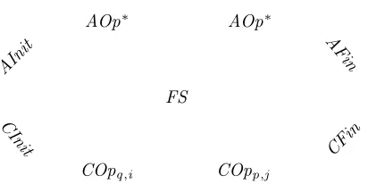
allow for a step-by-step comparison treating initialization, the operations and finalization separately. Simulations come in two flavors, forward and backward simulation. Together, these are sound and jointly complete as a methodology for verifying refinements [de Roever and Engelhardt 1998; Derrick and Boiten 2001]. In most standard applications of refinement, observation is the input/output of the data type [Woodcock and Davies 1996], however, in the context of verifying linearizability, our notion of observable behavior is the histories. In the next sections we will show that the concrete data type is a weak data refinement of the abstract data type using a finalization operation extracting histories. Here, we first of all define a notion of forward and backward simulation appropriate for weak data refinement. Figure 1 shows the proof obligations for a forward simulation. As with all simulations, we need to find an abstraction (or retrieve) relation FS relating states of the concrete and the abstract data type, and show that initialization, finalization and operations of the concrete data type can be forward simulated by the abstract data type (in the sense that the diagrams commute).
Definition3.6 (Forward simulation). Let A = (AState,Obs,AInit,(AOpp,i)p∈P,i∈I,
AFin) and C = (CState, Obs, CInit, (COpp,j)p∈P,j∈J, CFin) be two data types with
finalization. A relation FS :AState ↔CState is aforward simulation from A to C if the following three conditions hold:
— Initialization:CInit ⊆AInito 9FS, — Finalization:FS o
9CFin ⊆AFin, — Correctness:∀p∈P,j ∈J •FSo
9COpp,j ⊆AOp
∗o
9FS. 2
In the correctness condition we see that now one operation of the concrete data type can be matched by a (possibly empty) sequence of arbitrary abstract operations. We will use the term ”match” in the following to mean the (sequence of) abstract operations for some concrete operation during simulation, both for forward and backward. We sometimes also say that a concrete operation ismappedto some abstract operation, or a sequence of abstract operations.
C In
it CFin
AIn
it AF
in
COpp,j
COpq,i
AOp∗ AOp∗
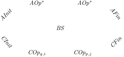
[image:14.612.205.412.94.190.2]BS
Fig. 2: Backward simulation conditions
Definition3.7 (Backward simulation). Let A = (AState,Obs,AInit,(AOpp,i)p∈P,i∈I,
AFin) and C = (CState,Obs,CInit,(COpp,j)p∈P,j∈J,CFin,GState) be two data types
with the same observations. A relation BS : AState ↔ CState is a backward simulation
fromC to Aif the following three conditions hold:
— Initialization:CInito
9BS ⊆AInit,
— Finalization:CFin ⊆BSo
9AFin, — Correctness:∀p∈P,j ∈J •COpp,j
o
9BS ⊆BS o
9AOp∗. 2
These two definitions give us a very general form of simulations which is needed for weak data refinement.
4. A SOUND AND COMPLETE PROOF TECHNIQUE
The starting point for our linearizability proofs is the following. Let ADT =
(AState,AInit,(AOpp,i)p∈P,i∈I) andCDT = (CState,CInit,(COpp,j)p∈P,j∈J) be two data
types, where setsI andJ are used to index the abstract and concrete operations, andP is a set of process identifiers. The function abs : J →I defines the correspondence between abstract and concrete operations, and is assumed to be total and surjective, and ann-to-1 mapping between concrete and abstract operations. Abstract operationsAOpp,i have input
and output denoted in? : INi and out! : OUTi, concrete operations COpp,j either have
an input in? : INabs(j) (invoking operations), or an output out? : OUTabs(j) (returning
operations) or no input and output at all.
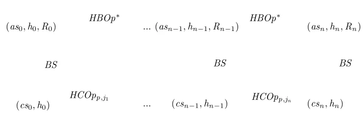
Our objective now is to show that we can always prove linearizability via a backward simulation, i.e.,CDT is linearizable with respect toADT if and only ifthere is a backward simulation between two specifically constructed data types, calledHBDTandHCDT. These data types first of all serve as a theoretical vehicle for proving the completeness result; however, they can also be used in linearizability proofs for case studies as we will see for the Herlihy-Wing queue.
In the following we will construct in total three data types fromADT and CDT, called
HADT, HBDT and HCDT.HADT and HBDT are constructed out ofADT andHCDT
out of CDT. We will speak of the data types ADT and HADT as residing on level A,
HBDT to constitute level B, and finallyCDT and HCDT to lay on level C. This idea of
levels originates from the usual way of drawing refinement relationships, where the abstract specification is drawn on top of the concrete specification. In our case, level B constitutes some intermediate level.
Each of the new data types will, in addition to the state we had so far, have histories – which the definition of linearizability is based on – in their state. Adding the history as an auxiliary variable does not change the runs of the data types. It enables to add a finalization
schema that compares the collected histories, implying thatHADT,HBDT andHCDT are
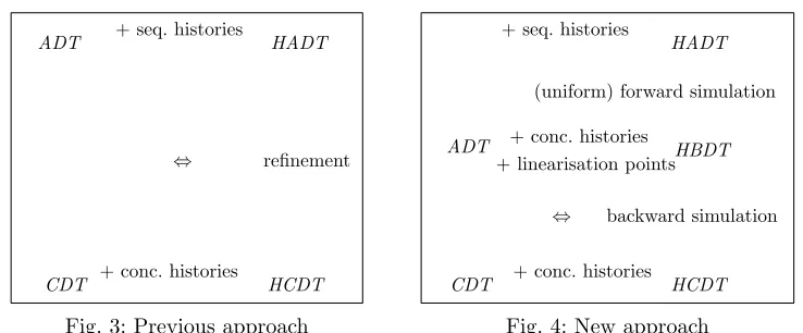
ADT HADT
HCDT ⇔
+ conc. histories CDT
[image:15.612.125.494.88.241.2]refinement + seq. histories
Fig. 3: Previous approach
HBDT + conc. histories
+ linearisation points ADT
⇔ backward simulation
CDT + conc. histories HCDT + seq. histories
HADT
(uniform) forward simulation
Fig. 4: New approach
4.1. Constructing our data types
Figure 3 shows our approach as detailed in previous papers. From a givenADT and CDT
we first of all constructed data typesHADT andHCDT which enhanced them with histories
and a generalized finalization operation returning histories. For these, we showed thatCDT
is linearizable toADT if and only if a refinement fromHADT toHCDT exists. This is the main result we proved in [Derrick et al. 2011a]. Proving refinement usually involved forward
andbackward simulations.
Here, we are now interested in proving completeness of backward simulation alone for
linearizability. To this end, we define the new intermediate specification HBDT (we can
think of these as forming three levels, and thus HBDT sits in between level ADT and
CDT, see Figure 4), which adds concurrency and a notion of linearization point to ADT.
It, however, does not yet resemble the concurrent implementation. Just likeHADT,HBDT
is constructed from the abstract data typeADT only. LevelBsplits the operations ofADT
into invocations, returns and an explicitlinearization operations, i.e., operations where the
effect on the data structure happens. The main result of this paper is now that CDT is
linearizable to ADT if and only if there is a backward simulation between HBDT and
HCDT. For the proof of this fact we need a further property of these three levels, namely
that therealwaysis a forward simulation betweenHADT andHBDT, i.e., even ifCDT is
not linearizable. The existence of this forward simulation justifies that we can safely work
withHBDT in our completeness theorem.
The result implies thatall linearizability proofs can in principle be done with backward simulation. However, it does not directly provide us with a technique for constructing these backward simulations for concrete examples. We next explain all levels and the forward and backward simulations in detail.
Abstract level. For our first level A we extend ADT with histories and
final-ization giving us a new data type HADT = (HAState,History, History × HAInit,
(HAOpp,i)p∈P,i∈I,HAFin). Basically, we extend the local state ofADT with a new variable
storing the current history of a run. States are thus of type (as,hs) where as is a state of
ADT and hsa sequential history.
HAState =b AState∧[hs : seqEvent]
Obs =b History
HAInit =b AInit∧[hs′: seqEvent |hs′ =h i]
HAOpp,i =b ∃in? :INi,out? :OUTi•
AOpp,i∧[hs,hs
′ : seqEvent |hs′=hsahinv(p,i,in?),ret(p,i,out!)i]
As in all following definitions, initialization ignores the input history: it is defined to relate any history to the initial states specified byHAInit ⊆History×Astate. Operations imme-diately add invocations and returns to the history, thus levelA is sequential. Furthermore note that the finalization does not return the sequential history itself but nondeterminis-tically returns a concurrent history which is linearizable into the sequential history. Thus the finalization here is consistent with the finalization of a concrete data type returning a concurrent history iff the concurrent history is linearizable wrt. the sequential history.
For future reference in simulations we define a predicatelinval(hs,as), that characterizes
possible final valuesas after running the operations of a sequential historyhs by
linval(hs,as)= (b hs,as)∈HAOp∗(|HAInit|)
The definition makes use of the Z operator R(|S |) returning the relational image of set
S under relation R.
Intermediate level.In the intermediate level B we use a variable R which takes sets of return events. The state of data typeHBDT is defined to be of type (as,h,R), whereasis a state ofADT,ha history andRa set of returns. This setRresembles the return events used in the linearizability definition to extend the current history (∃h0 : seqRet! • . . .). These
are the returns which have not happened so far but for which the effect of the operation has already taken place. Since we have an explicit formalization of linearization point inHBDT
(see next), it is easy to determine when such a return event has to be in the setR. In addition, we divide the abstract operations into invocation, return and linearization operations. Invocation of an operation from a processp can only occur if there is no pend-ing invocation of the same process in the history, returns can only occur when there is a pending invocation. The linearization operation, called Lin, is used to make the notion of “an operation taking effect” explicit. Thus the new operation Lin adds an appropriate re-turn event toR. So, invocations and returns just extend the histories, whereas linearization changes both the local stateAState of the data structure and adds an event to R.
This gives data type HBDT = (HBState,History,History ×HBInit,(Linp,i)p∈P,i∈I ∪
(Invp,i)p∈P,i∈I∪(Retp,i)p∈P,i∈I,HBFin) defined by
HBState =b AState∧[h: seqEvent,R:PRet]
Obs =b History
HBInit =b AInit∧[h=h i ∧R=∅]
Invp,i = [(¬ ∃b i
′
,in′•inv(p,i′,in′)∈pi(h))∧
∃in? :INi • as′=as∧R′=R∧h′=hahinv(p,i,in?)i]
Linp,i = [∃b in,out •inv(p,i,in)∈pi(h)∧(¬ ∃out2•ret(p,i,out2)∈R)∧
AOpp,i(in,as,as
′
,out)∧h′=h∧R′=R∪ {ret(p,i,out)}]
Retp,i = [∃b out! :Outi•ret(p,i,out!)∈R∧h
′=hahret(p
,i,out!)i ∧
R′=R\ {ret(p,i,out!)} ∧as′ =as]
HBFin =b HBState∧[H : seqEvent |H =h]
Again the initialization relation ignores the initial history. We defineHBOpto be the union relationSp∈P,i∈I(Linp,i∪Retp,i∪Invp,i) of all operations ofHBDT,Lin =b
S
p∈P,i∈ILinp,i
is all linearization operations, and similarly for Ret andInv.
Note that levelB is concurrent, i.e., produces concurrent histories. Note also that level
B is only derived from levelA, and uses the same index setI for operations.
Example: As an example we give a run of HBDT which resembles the concrete run given in Section 2. Note that there is more than one such run. Recall that the state is has,h,Ri
hh i,h i,∅i
−Inv3,enq(a)
−−−−−−→ hh i,hinv(3,enq,a)i,∅i
−Inv1,enq(b)
−−−−−−→ hh i,hinv(3,enq,a),inv(1,enq,b)i,∅i
−Inv2,deq()
−−−−−→ hh i,hinv(3,enq,a),inv(1,enq,b),inv(2,deq,)i,∅i
−Inv4,enq(c)
−−−−−−→ hh i,hinv(3,enq,a),inv(1,enq,b),inv(2,deq,),inv(4,enq,c)i,∅i
−Lin4,enq
−−−−→ hhci,hinv(3,enq,a),inv(1,enq,b),inv(2,deq,),inv(4,enq,c)i,{ret(4,enq,)}i
−Lin2,deq
−−−−→ hh i,h. . .i,{ret(4,enq,),ret(2,deq,c)}i
−Ret4,enq()
−−−−−→ hh i,h. . . ,ret(4,enq,)i,{ret(2,deq,c)}i −Lin3,enq
−−−−→ hhai,h. . . ,ret(4,enq,)i,{ret(2,deq,c),ret(3,enq,)}i
−Ret2,deq(c)
−−−−−−→ hhai,h. . . ,ret(4,enq,),ret(2,deq,c)i,{ret(3,enq,)}i
−Ret3,enq()
−−−−−→ hhai,h. . . ,ret(4,enq,),ret(2,deq,c),ret(3,enq,)i,∅i
−Lin1,enq
−−−−→ hha,bi,h. . . ,ret(4,enq,),ret(2,deq,c),ret(3,enq,)i,{ret(1,enq,)}i
−Ret1,enq()
−−−−−→ hha,bi,h. . . ,ret(4,enq,),ret(2,deq,c),ret(3,enq,),ret(1,enq,)i,∅i
2 Concrete level. In a third step we now construct level HCDT consisting of the con-crete operations in the concurrent implementation extended with histories. This is
sim-ilar to the extension HADT which we have already defined for ADT. One difference
here is that the finalization returns the history itself. In order to determine when to extend histories by inv’s or ret’s we classify all operations of the concrete data type into invocation, return or other operations. Therefore our final data type is defined as
HCDT = (HCState,History,History×HCInit,(HCOpp,j)p∈P,j∈J,HCFin) where
HCState=b CState∧[h: seqEvent]
Obs =b History
HCInit =b CInit∧[h′: seqEvent |h′ =h i]
HCFin=b HCState∧[H : seqEvent|H =h] and the operations are defined by
HCOpp,j =b
∃in? :INabs(j)•COpp,j ∧[h,h
′ : seqEvent |h′=hahinv(p
,abs(j),in?)i]
iffj is an invoke operation ∃out! :OUTabs(j)•COpp,j∧[h,h
′: seqEvent |h′=hahret(p,abs(j),out!)i]
iffj is a return operation
COpp,j∧[h,h
′: seqEvent |h′ =h]
otherwise
All operations of the embedded type now work on the concrete state plus the history.
Embedding an operation COpp,j that invokes an algorithm and has input in? gives an
operationHCOpp,j that adds a corresponding invoke event to the history, and similarly for
returning operations. All others leave the history unchanged. Again, as expected, levelC is concurrent.
Example:For the Herlihy-Wing queue we have invocation operationsenq0p anddeq0p and
return operations enq3p and deq6p for all p ∈ P. This gives the following examples of
enhanced concrete operations:
HCEnq0p =b ∃lv?•enq0p∧[h,h′: seqEvent |h′=hahinv(p,enq,lv?)i]
HCEnq1p =b enq1p∧[h,h′: seqEvent |h′=hi]
2
4.2. Soundness and Completeness Results
These definitions help us to establish the main result of the paper, namely that backward simulations are sound and complete for showing linearizability. So, for the constructed data types of levels A,B andC we will now show that
(1) there always exists a forward simulation fromHADT toHBDT(by showing thatInvp,i
and Retp,i in HBDT are matched by empty steps of HADT andLinp,i in HBDT by
HAOpp,i inHADT), and – the main result – that
(2) a backward simulation fromHCDT toHBDT exists if and only ifCDT is linearizable
with respect toADT.
Central to both proofs will be the notion of possibilities. Possibilities have already been introduced in [Herlihy and Wing 1990] as an alternative way of defining linearizability. A possibility is a triple consisting of a history h, a set of return events R and a state as. Intuitively,Poss(as,h,R) means that it is possible to reach abstract stateaswhen executing the history h assuming that all returns in R have taken place, i.e., these operations have already taken effect and have changed the state. In [Derrick et al. 2011a] there is a rule-based definition of possibilities, which exactly matches the way we construct the state of levelB. Thus we directly use it here.
Definition 4.1. A possibility is a reachable state of the B-level. Thus we define
Poss(as,h,R) by the following (remember from aboveHBOp is the union of all operations
in B) :
Poss(as,h,R)= (b as,h,R)∈HBOp∗(|HBInit |) 2
Note that the histories occurring in possibilities are concurrent. We get the following prop-erty of possibilities.
Proposition 4.2. Possibilities are prefix-closed: If Poss(as,h0ah,R) for some
his-tories h0,h, set of returns R and abstract state as, then there are as0 and R0, such that
Poss(as0,h0,R0)and HBOp∗((as0,h0,R0),(as,h0ah,R)).
Proof:Simple induction over the number of operation applications necessary to reach the final state (as,h0ah,R), since every operation adds at most one event and we start with
the empty history. Remark: This lemma is already known from [Herlihy and Wing 1990],
p. 487. 2
Possibilities and linearizability are equivalent in the following sense: Whenever we have a possibility (as,h,R), then we can arrange the return events inRinto some arbitrary order, append them tohand by this get a linearizable history. Conversely, if a concurrent history can be extended (with those returns for which the effect of the operation has already taken place) and is then linearizable, we also have a possibility for this history.
To formally state this close connection, we need a definition to relate return event sets and histories. We let setof(h) stand for the set of events occurring in h. We then define
R =setof(h) to be true iff h is a (duplicate free) sequence that contains the same set of events asR. The following theorem just formalizes one direction, namely that linearizability implies possibilities. (Recall thatcomplete(hah0,hs) removes all pending invocations from
(hah0,hs), andlin is the linearizable predicate.)
Theorem 4.3. Let h be a history and as an abstract state. Then the following holds.
∃h0,hs•lin(complete(hah0),hs)∧linval(hs,as)∧h0⊆seq Ret!
This theorem is very similar to Theorem 10 of [Herlihy and Wing 1990]; we have given a
proof in [Derrick et al. 2011a]. 2
With these definitions and results at hand, we can formulate and prove our first result about the existence of a forward simulation between levelsA andB.
Theorem 4.4. Let HADT and HBDT be the data types of levels A and B as defined
in Section 4.1. Then there exists a forward simulation from HADT to HBDT .
Proof:We construct a forward simulation relationFS from HADT to HBDT. Note that states of HADT are of the form (as,hs) and those of HBDT of type (bs,h,R). We first
define the forward simulation relation we will use as the following:
FS ={((as,hs),(bs,h,R))|as=bs∧Poss(bs,h,R)∧linval(hs,as)∧
∀h0•R=setof(h0)⇒lin(complete(hah0,hs)}
remembering that the predicate linval(hs,as) characterizes possible final values as after running the operations of a sequential historyhs.
We need to show that this is indeed a forward simulation.
Initialization. Straightforward asHBInit(bs,h,R) impliesAInit(bs) and the definition
of HBDT immediately gives us Poss(bs,h,R). The rest then follows by the fact that
lin(h i,h i) holds.
Finalization. Straightforward: by definition of FS we know that for all
((as,hs),(bs,h,R))∈FS the historyh is linearizable intohs.
Correctness. Let ((as,hs),(bs,h,R)) ∈ FS. We split the correctness proof into three
cases covering invoke, return and linearization operations.
(1) Assume the concrete operation in level B to be executed is an invoke. Hence
(bs,h,R) −Invp,i
−−−→ (bs,hahinv(p,i,in?)i,R) for some input in?. For the level A
we choose an empty (skip) step. Thus we need to show that ((as,hs),(bs,h a
hinv(p,i,in?)i,R))∈FS:
— (i)as=bs still holds,
— (ii)Poss(bs,hahinv(p,i,in?)i,R) holds by definition ofPoss,
— (iii)∀h0•R=setof(h0⇒lin(complete(hahinv(p,i,in?)iah0,hs)) holds since
complete is removing the (new) pending invoke, — (iv)linval(hs,as) is still true.
(2) Assume the concrete operation in level B to be executed is a return. Hence
(bs,h,R) −Retp,i
−−−→ (bs′,h′,R′) where (bs′,h′,R′) is (bs,h ahret(p,i,out!)i,R \
{ret(p,i,out!)}) for some output out!. For the level A we again choose an empty
(skip) step. Thus we need to show that ((as,hs),(bs,h a hret(p,i,out!)i,R \
{ret(p,i,out!)}))∈FS:
— (i)as=bs still holds,
— (ii)Poss(bs,hahret(p,i,out!)i,R\ {ret(p,i,out!)}) by definition ofPoss,
— (iii) We need to show∀h0′ •R′=setof(h0′)⇒lin(complete(h′ah0′,hs)). We take
an arbitrary h′
0. From this we construct a sequenceh0 =b hret(p,i,out!)iah0′.
For this we have R=setof(h0), hence lin(complete(hah0,hs)). The fact that
hah0=h′ah′
0 gives us the desired result.
— (iv)linval(hs,as) is still true.
(3) Assume the concrete operation in level B to be executed is a
lineariza-tion step. Hence (bs,h,R) −Linp,i
−−−→ (bs′,h′,R′) where for bs′ we know that
AOpp,i(in?,bs,bs
{ret(p,i,out!)}. Now we choose AOpp,i as corresponding abstract step and this
brings the abstract state toas′ =b bs′ andhs′ =b hsahinv(p,i,in?),ret(p,i,out!)i.
Again we get as′ =bs′,Poss(bs′,h′,R′) and linval(hs′,as′) by definition. The in-teresting part is again the requirement about lin.
Since we have taken a Lin-step, inv(p,i,in) ∈ pi(h) must hold, so h = h1a
hinv(p,i,in)iah2 for some h1 and h2. Also AOpi(in,as,as′,out) and R′ =R∪
ret(p,i,out) must be true to havePoss(as′,h′,R′).
We seths′=b hsahinv(p,i,in),ret(p,i,out)i, and have to provelin(complete(h′a
h0′,hs′)) for every h0′ that satisfies R′ = setof(h0′). The latter implies h0′ = h1′ a
hret(p,i,out)iah2′, since ret(p,i,out) ∈ h0′, and we can choose h0 =b h1′ ah2′ in
the induction hypothesis. Sinceh0satisfiesR=setof(h0), we getlin(complete(ha
h0),hs) andlinval(hs,as).
Now,complete(hah0) =complete(h1ah2ah′
1ah2′) sinceinv(p,i,in) is a pending
invoke inhah0, that is dropped by the complete-function. The induction hypothesis
therefore gives an order-preserving bijection between complete(h1ah2ah1′ ah2′)
andhs. This bijection can be extended to one between
complete(h′ah′
0) =complete(h1ahinv(p,i,in)iah2ah1′ ahret(p,i,out)iah2′)
and hs′ as required to prove lin. This is done by adding a mapping between the two additional eventsinv(p,i,in) andret(p,i,out) (the technical details are quite
complex, sincepositionsmust be mapped, which change by one for events between the invoke and the return, and by two for events inh2′). The new mapping is order preserving, since no operation is started inh′ah′
0after the returnret(p,i,out).
2
As a corollary we now get the other connection between possibilities and linearizability (a strengthened version of Theorem 9 in [Herlihy and Wing 1990]):
Corollary 4.5. Let h be a history, R a set of return events and as an abstract state.
Then
Poss(as,h,R)⇒
∃hs• ∀h0•R=setof(h0)⇒lin(complete(hah0),hs)∧linval(hs,as)
Proof: AssumingPoss(as,h,R), the forward simulation asserts the existence of (hs,as′)
with FS((hs,as′),(h,as,R)). Expanding the definition ofFS gives the desired conclusion. 2
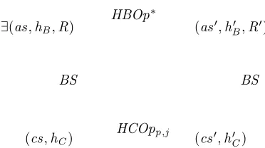
Our second result is the one that links the intermediate to the concrete level. Here, we can show that linearizability is equivalent to the existence of a backward simulation. This is our soundness and completeness result for linearizability.
Theorem 4.6. Let HBDT and HCDT be the data types of levels B and C as defined
above, and let ADT and CDT be the original data types we started with. Then CDT is linearizable with respect to ADT if and only if there is a backward simulation between HCDT and HBDT .
Proof:We have to prove two parts: (a)Soundness:the existence of an arbitraryBS being
a backward simulation between HBDT and HCDT implies that CDT linearizable wrt.
ADT, and (b)Completeness: CDT linearizable wrt.ADT implies that there is a backward
(cs′,h′ C)
BS
(cs,hC)
(as′,hB′ ,R′)
BS
HCOpp,j
HBOp∗
[image:21.612.223.409.89.193.2]∃(as,hB,R)
Fig. 5: Correctness rule for backward simulation
Part (a): Assume there is a backward simulation BS between HCDT and HBDT,
and assume an arbitrary run of HCDT is given, that starts with (cs0,h0) such
that cs0 is initial and h0 = hi, goes through (csi,hi) for 0 ≤ i ≤ n and
ends in (csn,hn). We have to prove that hn is a linearizable history. The
finaliza-tion condifinaliza-tion ensures that there is a state (asnhn,Rn) of HBDT with the same
hn. Now the correctness condition of backward simulation (see Fig. 5) guarantees
that (asn−1,hn−1,Rn−1) can be found with BS((csn−1,hn−1),(asn−1,hn−1,Rn−1)) and
HBOp∗((asn−1,hn−1,Rn−1),(asn,hn,Rn)). Iterating the construction (see Fig. 6) gives
states (asi,hi,Ri), all linked via BS (and therefore all having the correct hi because
of finalization) such that HBOp∗((asi,hi,Ri),(asi+1,hi+1,Ri+1). Altogether we have
HBOp∗((as
0,h0,R0),(asn,hn,Rn). SinceHCInit(cs0,h0) holds, the initialization condition
impliesHBInit(as0,h0,R0). Together this implies that (asn,hn,Rn) is a reachable state of
HBDT, i.e.,Poss(asn,hn,Rn). Finally, Corollary 4.5 gives the desired linearizability ofhn.
Part (b): assumeCDT is linearizable wrt.ADT. We prove thatBS defined by
BS ={((cs,hC),(as,hB,R))|Poss(as,hB,R)∧hB=hC∧(hB=h i ⇒AInit(as))}
is always a backward simulation.
Initialization. if HCInit(cs,hC) and BS((cs,hC),(as,hB,R)) then we know that
hB = hC and thus empty, and furthermore AInit(as) and R = ∅ which implies
HBInit(as,hB,R).
Correctness. requires that given a concrete transition (cs,hC) − HCOpp,i
−−−−−→ (cs′,h′ C)
and an abstract state (as′,hB′ ,R′) we need to find a state (as,hB,R) such that
((cs,hC),(as,hB,R)) ∈ BS and (as,hB,R) −HBOp
∗
−−−−→ (as′,hB′ ,R′) (see Figure 5).
Es-sentially this follows from Proposition 4.2: We know thathC is a prefix ofhC′ (histories
are only extended by operations), thus by prefix-closedness of possibilities there must be some possibility Poss(as,hC,R) such that HBOp∗((as,hC,R),(as′,hC′ ,R′)). If hC
is moreover empty,as has to be an initial state since possibilities with empty histories always contain an initial state. Thus we getBS((cs,hC),(as,hC,R)).
Finalization. IfHCFin((cs,hC),hC) then by linearizability of CDT wrt.ADT we get
the following: ∃hS such that ∃h0 ∈ seqRet! • lin(complete(hC ah0),hS)∧ ∃as •
linval(hS,as). By Theorem 4.3 we getPoss(as,hC,setof(h0)). Hence this has to be a
state ofHBDT. Furthermore, if hC (and thushB) is empty, we have AInit(as) as the
initial state is the only one which belongs to a possibility with an empty history, and
thusBS((cs,hC),(bs,hC,setof(h0)). 2
(csn,hn)
BS
(asn,hn,Rn)
BS
HCOpp,jn
HBOp∗
(cs0,h0)
(as0,h0,R0)
HBOp∗
HCOpp,j1
BS
...
...
(asn−1,hn−1,Rn−1)
[image:22.612.131.500.81.204.2](csn−1,hn−1)
Fig. 6: Composing commuting bw. sim. diagrams
8 on related work. In summary, Theorem 4.6 shows, that for linearizability, the only history variable ever needed is the history needed to define linearizability (i.e., possibilities) itself.
The backward simulationBS of the completeness proof is in some sense amaximal back-ward simulation, since every other backback-ward simulationB will satisfy
B((cs,hB),(as,hC,R))→BS((cs,hB),(as,hC,R))
for all reachable states (cs,h) as the soundness proof shows. BS is also completely
inde-pendent of the concrete statecs. In applications we will of course make use ofcs to define
smaller simulations: relating fewer states (but not too few!) makes the proof of the main correctness condition for backward simulation easier, since fewer commuting diagrams have to be completed in the correctness condition.
Since any backward simulation must always keep the concrete and the abstract history
identical, the “matching” sequence HBOp∗ used in the commuting diagrams of Fig. 5 can
be specialized. For an invoking operation the sequence must have the formLin∗o 9Inv
o 9Lin∗, (recall, that Lin is the union of all linearization operations Linp,i; similarly for Inv and
Ret), since only sequences of that type will update the history by adding one invoke event.
For a returning operation the matching sequenceHBOp∗ must beLin∗o
9Ret o 9Lin
∗. All
other operations can only correspond to a sequenceLin∗ of linearization points.
In the case study we will map only internal operations (i.e., ones that do not change the history) to Lin-steps. This seems to be possible in general, when invoke and return operations only copy input/output to/from local buffers, and when all algorithms have at least one step between invoke and return. For the maximal backward simulation it is possible to show that it executes all linearization points as early as possible, i.e., directly with invoking operations. This can be shown based on the following observation.
Proposition 4.7. For processes p,q ∈P , p 6=q, and arbitrary operation indices i,j ,
the operations of HBDT satisfy Linp,i
o
9Invq,j =Invq,j o
9Linp,i and Linp,i o
9Retq,j =Retq,j o 9Linp,i
Linearization steps commute with both invoke and return steps of other processes.
Therefore we can strengthen the completeness part of theorem 4.6 above to:
Theorem 4.8. If CDT is linearizable with respect to ADT , then it is possible to find
a backward simulation between HBDT and HCDT such that in the correctness condition
HCOpp,j o
9BS ⊆BS o 9HBOp
∗
the abstract operation sequence HBOp∗ can be strengthened to:
— Retp,i, when the concrete operation is a return operation and abs(j) =i
— Invp,i o
9(skip∪(Linp,i o 9Lin
∗))for invoke operations