City, University of London Institutional Repository
Citation:
Aboukhedr, M., Georgoulas, A., Marengo, M., Gavaises, M. ORCID: 0000-0003-0874-8534 and Vogiatzaki, K. (2018). Simulation of micro-flow dynamics at low capillary numbers using adaptive interface compression. Computers & Fluids, 165, pp. 13-32. doi: 10.1016/j.compfluid.2018.01.009This is the accepted version of the paper.
This version of the publication may differ from the final published
version.
Permanent repository link:
http://openaccess.city.ac.uk/19881/Link to published version:
http://dx.doi.org/10.1016/j.compfluid.2018.01.009Copyright and reuse: City Research Online aims to make research
outputs of City, University of London available to a wider audience.
Copyright and Moral Rights remain with the author(s) and/or copyright
holders. URLs from City Research Online may be freely distributed and
linked to.
Accepted Manuscript
Simulation of micro-flow dynamics at low capillary numbers using adaptive interface compression
M. Aboukhedr, A. Georgoulas, M. Marengo, M. Gavaises, K. Vogiatzaki
PII: S0045-7930(18)30009-4
DOI: 10.1016/j.compfluid.2018.01.009
Reference: CAF 3692
To appear in: Computers and Fluids
Received date: 12 July 2017
Revised date: 15 November 2017
Accepted date: 13 January 2018
Please cite this article as: M. Aboukhedr, A. Georgoulas, M. Marengo, M. Gavaises, K. Vogiatzaki, Simulation of micro-flow dynamics at low capillary numbers using adaptive interface compression,
Computers and Fluids(2018), doi:10.1016/j.compfluid.2018.01.009
ACCEPTED MANUSCRIPT
Highlights1
• Multiphase flow solver using adaptive compression scheme has been introduced.
2
• Wide range of conditions using well-established benchmark cases has been tested.
3
• The adaptive compression facilitates simulating flows at law capillary numbers.
4
• The adaptive nature of the coef. counter balances the need for very fine grids.
5
• Using the mentioned method gives accurate results in estimating bubble formation.
ACCEPTED MANUSCRIPT
Simulation of micro-flow dynamics at low capillary numbers using adaptive
7interface compression
✩8
M. Aboukhedra,∗, A. Georgoulasb, M. Marengob, M. Gavaisesa, K. Vogiatzakib 9
aDepartment of Mechanical Engineering, City, University of London, UK
10
bSchool of Computing, Engineering and Mathematics, Advanced Engineering Centre, University of Brighton, Brighton, UK
11
Abstract
12
A numerical framework for modelling micro-scale multiphase flows with sharp interfaces has been
13
developed. The suggested methodology is targeting the efficient and yet rigorous simulation ofcomplex
14
interface motion at capillary dominated flows (low capillary number). Such flows are encountered in
vari-15
ous configurations ranging from micro-devices to naturally occurring porous media. The methodology uses
16
as a basis the Volume-of-Fluid (VoF) method combined with additional sharpening smoothing and filtering
17
algorithms for the interface capturing. These algorithms help the minimisation of the parasitic currents
18
present in flow simulations, when viscous forces and surface tension dominate inertial forces, like in porous
19
media. The framework is implemented within a finite volume code (OpenFOAM) using a limited
Multi-20
dimensional Universal Limiter with Explicit Solution (MULES) implicit formulation, which allows larger
21
time steps at low capillary numbers to be utilised. In addition, an adaptive interface compression scheme
22
is introduced for the first time in order to allow for a dynamic estimation of the compressive velocity only
23
at the areas of interest and thus has the advantage of avoiding the use of a-priori defined parameters. The
24
adaptive method is found to increase the numericalaccuracy and to reduce the sensitivity of the
methodol-25
ogy to tuning parameters. The accuracy and stability of the proposed model is verified against five different
26
benchmark test cases. Moreover, numerical results are compared against analytical solutions as well as
27
available experimental data, which reveal improved solutions relative to the standard VoF solver.
28
Keywords: CFD, interFoam, two-phase flows, microfluidics, surface tension forces, parasitic currents,
29
micro-scale modelling
30
✩This document is a collaborative effort
∗Corresponding author
ACCEPTED MANUSCRIPT
List of Nomenclature
u Velocity
p Pressure
pc Capillary pressure pd Dynamic pressure f External forces fg Gravitational forces fs Surface tension force
ρ Density
µ Dynamic viscosity
ur,f Relative velocity at cell faces
σ Surface tension
φf Volumetric flux
φc Compression volumetric flux
φ Capillary flux
φthreshold Threshold volumetric flux Vi Volume per grid cell Sf Outward-pointing face area
κ Interface curvature
κf Filtered interface curvature calculated based on smooth functionαsmooth
κs,i+1 Smooth interface curvature calculated based on smooth functionκf
κf inal Weighted interface curvature calculated based on smooth functionκs,i
ηs Normal vector to the interface
δs Dirac delta function
α Volume fraction
αsmooth Volume fraction using Laplacian formulation
αsh Sharp inductor function
Ccompr. Constant interface compression coefficient Cadp Adaptive interface compression
Csh Sharpening coefficient Uf filtering coefficient
hηsif Face centred normal vector
h5αif Volume fraction interpolated from cell centre to face centre
δn Small value
1. Introduction
31
Flows through ”narrow passages” such as micro-channels or pore-scale flows whose dimensions are
32
less than O(mm) and greater than O(µm) differ from their macroscopic counterparts at important aspects:
33
the small size of the geometries makes molecular effects such as wall slip or wettability more important,
ACCEPTED MANUSCRIPT
while amplifies the magnitudes of certain ordinary continuum effects associated with strain rate and shear35
stress. Such flows are present in various natural formations (rocks and human organs) as well as man-made
36
applications (micro-conductors, micro-emulsions, etc.). Thus, microscale physics attracts the interest of
37
various disciplines including cosmetic and pharmaceutical industries as well as biomedical and petroleum
38
engineering. For more details on the application of microscale geometries, the reader is referred to [1].
39
Among all these applications transportation of droplets in microchannels at low Capillary (Ca= µuσ)
num-40
bers has attracted the interest of researchers from the theoretical and experimental point of view [2, 3, 4].
41
For example, understanding the dynamics of immiscible fluids in micro-devices can facilitate the creation
42
of monodisperse emulsions. Droplets of the same size move with low velocities through microchannel
43
networks and are used as micro-reactors to study very fast chemical kinetics [5]. Another example of low
44
Ca flow dynamics in micro-scale can be seen at trapped oil blobs in porous reservoirs. Understanding the
45
trapping flow dynamics at the pore scale level can be the key to minimising the trapping of a non-wetting
46
phase and enhancing recovery systems of hydrocarbons, [6]. Although a large number of methods has been
47
developed for simulating multiphase flows at macro-scale including the well known Level Sets (LS) [7] and
48
Volume of Fluid (VoF) methods [8], the extension of these methods to micro-scale is not always
straightfor-49
ward. The main weakness of the LS methods is that they do not preserve mass. As a result, poorly resolved
50
regions of the flow are typically susceptible to mass loss behaviour and loss of signed distance property due
51
to advection errors. Various modification have been suggested focusing on solving the conservation issues
52
[9], extending the method to high Reynolds numbers [10] and to unstructured meshes [11, 12]. While using
53
a re-initialization procedure as discussed by [13] is a solution to the mass conservation issue, it increases
54
the computational cost and creates an artificial interface displacement that may affect mass conservation,
55
see the review by Russo and Smereka [14] for details. Similarly the VoF method is based on the numerical
56
solution of a transport equation that distinguishes the two fluids in the domain, and it represents the volume
57
percentage of each fluid phase in each cell over the total volume of the cell. The interface between the two
58
phases is defined in the cells where the VoF function takes a value between (0, 1). In incompressible flows,
59
the mass conservation is achieved by using either a geometrical reconstruction coupled with a geometrical
60
approximation of the volume of fluid advection or a compressive scheme as discussed by Rusche [15] and
61
implemented by Weller et al. [16]. The VoF method has been the most widely used interface capturing
ACCEPTED MANUSCRIPT
method due to ease of implementation as reviewed by W¨orner [2].63
Within the VoF framework two commonly used methods for interface representation exist: (a) a
com-64
pressive method and (b) a geometric method. Both VoF methods are used in order to calculate the discrete
65
volume fraction of each phase within a cell, which is then transported based on the underlying fluid
ve-66
locity. Compressive VoF methods discretise the partial differential equation describing the transport of the
67
volume fraction of each phase using algebraic differencing schemes [17, 18]. The key for the accuracy of
68
these methods is that, in order to keep the interface sharp and without distortion, the temporal and spatial
69
discretisation should be performed using higher order schemes and careful tuning. Otherwise the method
70
may suffer from excessive diffusion of the interface region which also affects the calculation of the interface
71
curvature and the normal interface vectors. Park et al. [19] and Gopala and van Wachem [20] showed the
72
compressive VoF methods capabilities of advecting sharp interface, and they also underlined the difficulties
73
in retaining the shape and sharpness of the interface. Using a geometric method, an explicit
representa-74
tion of the interface is advected, reconstructed from the VoF volume fraction field. The piecewise linear
75
methods so-called (PLIC) is the most developed reconstruction method found in the literature [21, 22].
Ge-76
ometric methods advect the interface very accurately, but their main drawback is their complexity for 3D
77
applications, in particular when used in conjunction with an unstructured mesh [23].
78
Recently, the coupling between VoF and LS, the so-called Coupled Level Set Volume Of Fluid (CLSVoF)
79
method [24] has also received significant attention since it combines the advantages of both methods, i.e.,
80
the VoF mass conservation and the LS interface sharpness [24, 25] . On the downside, this approach also
81
combines the weaknesses of each method since techniques to keep the VoF interface sharp and reinitialise
82
the distancing function are needed. Based on various published results for both methods [20, 26, 27, 28] the
83
existent frameworks reviewed in the previous paragraph - regardless of the various modifications available
84
- still suffer from their inherent severe drawbacks. These drawbacks are more pronounced in low Ca flows,
85
and, as discussed in detail in Popinet and Zaleski [29], Tryggvason et al. [30] and Bilger et al. [31], stem
86
from the fact that sharp discontinuities such as interfaces are represented by finite volume integrals [8]. The
87
most common issue is that in all implicit interface capturing methods, the interface location is known by
88
defining the normal and the curvature implicitly.For the VoF methods ,in particular, which are based on the
89
representation of the discontinuous interface with continuous colour function, the calculation of the
ACCEPTED MANUSCRIPT
ties of each phase is possible, given an accurate numerical scheme for solving the colour function transport91
equation is available. However, the accuracy of the calculated interface curvature (that is then required
92
for the calculation of the capillary pressure force) depends on determining the derivative of the introduced
93
discontinuous colour function, which is considered to be difficult from a numerical point of view, and may
94
leads to numerical instabilities [32].
95
An additional issue is the generation of non-physical velocities at the interface which are known as
96
”spurious” or ”parasitic” currents. The primary sources of spurious currents have been identified as the
97
combination of inaccurate interface curvature and lack of a discrete force balance as discussed by Francois
98
et al. [33].It should be stressed that the local force imbalance between the capillary pressure and the pressure
99
arising from the normal component of the surface tension force vectors (due to the imprecise evaluation of
100
the local curvature) can create the non-physical velocities, (spurious currents”) which are commonly small
101
in absolute values in inertia dominated flows, but become very problematic in capillary dominated flows.
102
Numerical challenges related to the advection of the interface in the context of VoF are well documented
103
by Tryggvason et al. [30]. Intrinsic to the method, regardless if geometric reconstruction or interface
com-104
pression is used, is the numerical diffusion of the interface, which is highly dependent on the mesh size [18].
105
The numerical diffusion can be reduced by using a geometrical reconstruction coupled with a geometrical
106
approximation of the VoF advection as discussed by Roenby et al. [34]. Alternatively, using a compressive
107
algorithm, the convective term of the VoF equation can be discretised using a compressive differencing
108
scheme designed to preserve the interface sharpness. Examples include the HRIC by Muzaferija and Peric
109
[35], or the compressive model available within OpenFoam [16]. Compression schemes do not require any
110
geometrical reconstruction of the interface and extension to three dimensions and unstructured meshes is
111
straightforward. However, compression schemes are not always sufficient to eliminate numerical diffusion
112
completely and additional treatment is needed [36].
113
Various remedies that still have room for development have been suggested, and they can be
sum-114
marised as following: (i) ensuring an accurate balance between local pressure and surface tension gradient.
115
In Francois et al. [33] a cell-centered framework has been introduced. It is demonstrated that this algorithm
116
can achieve an exact balance of between local pressure and surface tension gradient using structured mesh.
117
Moreover, Francois et al. [33] and [37] discussed the origin of spurious currents within the introduced
ACCEPTED MANUSCRIPT
balanced-force flow algorithms, as they highlighted the deficiencies introduced at the interface curvature119
estimation. (ii) sharp representation of the interface, with accurate curvature estimation and introduction
120
of a so-called ”compression velocity” to damp diffusion. Ubbink and Issa [18] introduced the compressive
121
discretisation scheme so-called Compressive Interface Capturing Scheme for Arbitrary Meshes CICSAM
122
that makes a use of the normalised variable diagram concept introduced by Leonard [38]. Popinet [39]
123
generalised a height-function and CSF formulations to an adaptive quad/octree discretisation to allow
re-124
finement along the interface for the case of capillary breakup of a three-dimensional liquid jet. Moreover,
125
[39] discusses the long-standing problem of ”parasitic currents” around a stationary droplet in contrast to
126
the recent study of Francois et al. [33], where the issue is shown to be solved by the combination of
appro-127
priate implementations of a balanced-force CSF approach and height-function curvature estimation. (iii)
128
implicit or semi-implicit treatment of surface tension, Denner and van Wachem [40] reviewed the time-step
129
requirements associated with resolving the dynamics of the equations governing capillary waves, to
deter-130
mine whether explicit and implicit treatments of surface tension have different time-step requirements with
131
respect to the (1) dispersion of capillary waves, and (2) the formulation of an accurate time-step criterion for
132
the propagation of capillary waves based on established numerical principles. The fully-coupled numerical
133
framework with implicit coupling of the governing equations and the interface advection, and an implicit
134
treatment of surface tension proposed by [40] was used to study the temporal resolution of capillary waves
135
with explicit and implicit treatment of surface tension.
136
In the present work, a new framework for modelling immiscible two-phase flows for low Ca applications
137
dominated by surface tension is suggested. The standard multiphase flow solver of OpenFOAM 2.3x has
138
been extended to include sharpening and smoothing interface capturing techniques suitable for low Ca
139
numbers flow. In addition a new generalised methodology that utilises an adaptive interface compression is
140
introduced for the first time.While existing compressionschemes are based on an a priori tuned parameter,
141
which is typically kept constant throughout the simulations, in the present study compression isactivated
142
only in areas that the interface is prone todiffusion and the parameter is thus defined adaptively. This
143
adaptive scheme is proved to limit the interface diffusion and to keep parasitic currents to minimal levels
144
while reducing the computational time. The proposed framework for interface advection aspires to offer
145
better modelling of flows in microscale that up to date have been proven problematic. The paper is structured
ACCEPTED MANUSCRIPT
as following: Initially the numerical framework underlining the modifications suggested over the traditional147
VoF methodology in order to achieve better representation of the interface is introduced. The effect of
148
each parameter used in the proposed framework is then evaluated individually based on a wide range of
149
benchmark cases. The first test case refers to single and multiple droplet relaxations in a zero velocity field,
150
aiming to assess the capability of the framework to damp spurious currents using various combination of
151
control parameter. The evaluation of the solver for an advection test using the Zalesak disk [41] is also
152
presented followed by results relevant to the motion of circle in a vortex field (Roenby et al. [34], Rider and
153
Kothe [42]). Finally, a numerical study of the generation of bubbles in a T-junction is studied to evaluate
154
the introduced framework insimulating more complex two-phase flows at a low Ca numbers.
155
2. Numerical method
156
The method presented in this section is implemented within the open source CFD toolkit OpenFOAM
157
[43]. An incompressible and isothermal two-phase flow with constant phase densitiesρ1 andρ2 and vis-158
cositiesµ1 andµ2 is considered. The two phases are treated as one fluid and a single set of equations is 159
solved in the entire computational domain. The volume fraction,αof each phase within a cell is defined 160
by an additional transport equation. The formulation for the conservation of mass and momentum for the
161
phase mixture is given by the following equations:
162
∇ ·u=0 (1)
D
Dt(ρu)=∇ ·T− ∇p+ f (2)
where u is the fluid velocity, p is the pressure and ρ is the density. The pressure-velocity coupling is 163
handled using the Pressure-Implicit with Splitting Operators(PISO) method of [44, 45]. The term∇ ·T =
164
∇ ·(µ∇u)+∇u· ∇µ is the viscous stress tensor. The term f = fg + fs corresponds to all the external
165
forces, i.e. fg = ρgis the gravitational force and fsrepresents the capillary forces for the case of constant
166
surface tension coefficientσ. The global properties are weighted averages of the phase properties through
167
the volume fraction value that is calculated in each cell:
ACCEPTED MANUSCRIPT
ρ=ρ1+(ρ2−ρ1)α (3)
µ=µ1+(µ2−µ1)α (4)
The sharp interfaceΓ represents a discontinuous change of the properties of the two fluids. The surface
169
tension force must balance the jump in the stress tensor along the fluid interface. At each time step, the
170
dynamics of the interface are determined by the Young-Laplace balance condition as;
171
∆Pexact =σκ (5)
accounting for a constant surface tension coefficientσalong the interface. The termκrepresents the
inter-172
face curvature. The term on the right-hand side of Eq. 5 is effectively the source term in the Navier–Stokes
173
equations for the singular capillary force, that is only present at the interface. In the proposed numerical
174
method, the Continuum Surface Force (CSF) description of Brackbill et al. [8] is used to represent the
175
surface tension forces in the following form:
176
fs=σκf inalδs (6)
where the termκf inalrepresents the interface curvature at the final stage of smoothing as discussed in section 177
2.2,δs is a delta function defined on the interface, andηs is the normal vector to the interfaceαsmoothas 178
discussed in section 2.2 and is calculated by the following equation:
179
ηs= ∇αsmooth
|∇αsmooth| (7)
The termsδsandκf are associated with the artificially smoothed and sharpened indicator function fields that
180
will be discussed in details in the following section. In the VoF method, the indicator functionαrepresents
181
the volume fraction of one of the fluid phases in each computational cell. The indicator function evolves
182
spatially and temporally according to an advection transport equation of the following general form:
ACCEPTED MANUSCRIPT
∂α
∂t +∇ ·(αu)=0 (8)
Ideally, the interface between the two phases should be massless since it represents a sharp discontinuity.
184
However, within VoF formulation the numerical diffusion of Eq. 8 results in values ofαthat vary between
185
0 and 1.
186
The framework described above reflects the generalised framework of VoF methods that has been used in
187
an extensive range of two-phase flow problems with various adjustments and different degrees of success.
188
In the following sub-sections, an enhanced version of this basic framework is presented; its validity is
189
demonstrated through a range of benchmark cases that addresses some numerically challenging problems
190
reported in the relevant literature.
191
2.1. Adaptive Compression Scheme (Implicit)
192
To deal with the problem of numerical diffusion ofα, an extra compression term is used in order to limit 193
the convection term of Eq. 8 and consequently the thickness of the interface. Its numerical significance
194
relays on defining local flow (u) at the interface and preventing the increase of the gradient when alpha is
195
not constant, (i.e. the absolute value of the time derivative increases to counterbalance). The model for the
196
compression term makes use of the two-fluid Eulerian approach, where phase fraction equations are solved
197
separately for each individual phase, assuming that the contributions of two fluids velocities for the free
198
surface are proportional to the corresponding phase fraction. These phase velocities (u1andu2) relate with 199
the global velocity of the one fluid approachuas:
200
u=αu1+(1−α)u2 (9)
Replacing the above equation to Eq. 8 one gets:
201
∂α ∂t +∇ ·
n
αu1+(1−α)u2αo=0 (10)
Considering a relative velocity between the two phases (ur=u1-u2) which arises from the density and 202
viscosity stresses changes across the interface, the above equation can be written in terms of the velocity of
ACCEPTED MANUSCRIPT
the fluid:204
∂α
∂t +∇ ·(u1α)−∇ ·
n
ur,fα
(1−α)o
| {z }
compression term
=0 (11)
It should be noticed that in the above equation in the calculation of∇ ·(uα) term the unknown velocity 205
u1appears instead ofucreating an inconsistency with the basic concept of the one fluid approach. However, 206
since the compression term in reality is active only at the interface, continuity imposesu1=u2=uand thus 207
u1byucan be replaced. The discretisation of the compression term in Eq. 11 is not based directly on the 208
calculation of the relative velocityur at cell faces from Eq. 9 sinceu1 andu2 are unknown. It is instead 209
formulated based on the maximum velocity magnitude at the interface region and its direction, which is
210
determined from the gradient of the phase fraction:
211
ur,f =minCcompr.|φf| |Sf|,max
"|φ
f| |Sf|
#!
hηsif (12)
where the termφf is the volumetric flux andSf is the outward-pointing face area vector andhηsif is 212
the face centred interface normal vector.hif is used to denote interpolation from cell centres to face centres 213
using a linear interpolation scheme, and defined as following:
214
hηsif = h5αif
|h5αif +δn| ·Sf (13)
and
δn= 1e
−8 P
NVi
N
1/3 (14)
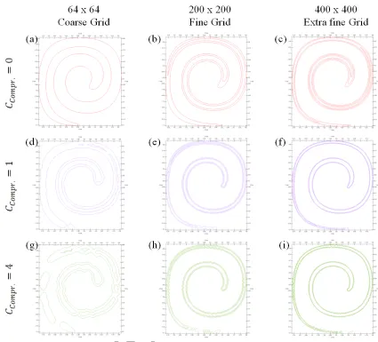
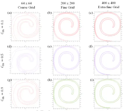
where δn is a small number to ensure that the denominator never becomes zero, N is the number of 215
computational cells, for each grid block i andViis its volume 216
The compressive term is taken into consideration only at the interface region and it is calculated in the
217
normal direction to the interface. The maximum operation in Eq. 12 is performed over the entire domain,
218
while the minimum operation is done locally on each face. The constant (Ccompr.) is a user-specified value,
219
which serves as a tuning parameter. Depending on its value, different levels of compression result are
220
calculated. For example, there is no compression for C= 0 while there is moderate compression with
ACCEPTED MANUSCRIPT
C≤1 and enhanced compression for C≥1. In most of the simulations presented here (Ccompr.) is taken as222
unity, after initial trial simulations. Values higher than unity in this case may lead to non-physical results.
223
Generally, this compression factor can take values from 0 (no compression) up to 4 (maximum compression)
224
as suggested in the literature; the selected values are case specific. To overcome the need for a priori tuning,
225
in the present numerical framework a new adaptive algorithm has been implemented that is based on the idea
226
of introducing instead of a constant value forCcompr.a dynamic oneCadpthrough the following relation:
227
Cadp =
− |uunn||∇· ∇αα|
(15)
φc =maxCadp,Ccompr.
|φf|
|S f| (16)
whereφcis the compression volumetric flux calculated,unrepresents each phase velocity normal to the
228
interface velocity. It is expressed as
229
un= U·nsx nsx|α−0.01| ∗ |0.99−α| (17)
The concept of usingun is shown in Fig. 1: when the interface profile becomes diffusive (wide)Cadp
value will increase accordingly in the zone of interest, while when the profile is already sharp and additional
compression is not necessaryCadpwill go to zero. Note that the compression term in Eq. 11 is only valid for
the cells at the interface. However, to solve Eq. 15, a wider region ofαis required. Therefore, the facial cell
field is extrapolated to a wider region using the expression (near interface) in Eq. 17 as (|α−0.01|∗|0.99−α|).
The new calculated, adaptive compression coefficientφcthen substitutes the originalCcompr.||φSff|| and Eq. 12
can be rewritten as:
ur,f =min φc,max
"|φ f|
|Sf| #!
hηsif (18)
The new equation still has a user defined valueCcompr.in cases when the adaptive coefficient is not sufficient.
230
2.2. Smoothing Scheme (Explicit)
231
By solving the transport equation for the volume fraction (Eq. 11), the value of (α) at the cell is updated.
232
In order to proceed with the calculation of the interface surface scalar fields for the calculation ofηsandκ,
ACCEPTED MANUSCRIPT
Figure 1: Schematic to represent the adaptive compressionCadpselection criterialinear extrapolation from the cell centres is used. At this stage, the value ofαsharply changes over a thin
234
region as a result of the compression step. This abrupt change of the indicator function creates errors in
235
calculating the normal vectors and the curvature of radius of the interface, which will be used to evaluate the
236
interfacial forces. These errors induce non-physical parasitic currents in the interfacial region. A commonly
237
followed approach in the literature to suppress these artefacts is to compute the interface curvature from
238
a smoothed function αsmooth, which is calculated by the smoother proposed by Lafaurie et al. [17] and
239
applied in OpenFOAM by Georgoulas et al. [46] and Raeini et al. [47]. The indicator function is artificially
240
smoothed by interpolating it from cell centres to face centres and then back to the cell centres recursively
241
using the following equation:
242
αi+1=0.5h(αi)c→fif→c−0.5αi (19)
Initial trial simulations indicated that the recursive interpolation between the cell and face centres can
243
be repeated up to three times, in order to prevent decoupling of the indicator function from the smoothed
244
function. After smoothing is implemented, the interface normal vectors in the cells in the vicinity of the
245
interface, are filtered using a Laplacian formulation. Equation 20 in Georgoulas et al. [46] is used in order
246
to transform the VOF function (αi+1) to a smoother function (αsmooth): 247
αsmooth=
Pn
f=1(αi+1)fSf Pn
f=1Sf
(20)
where the subscript denotes the face index (f) and (n) the times that the procedure is repeated in order
ACCEPTED MANUSCRIPT
to get a smoothed field. The value at the face centre is calculated using linear interpolation. It should249
be stressed that smoothing tends to level out high curvature regions and should therefore be applied only
250
up to the level that is strictly necessary to sufficiently suppress parasitic currents. After calculating the
251
(αsmooth), the interface normal vectors are computed using 7, and the interface curvature at the cell centres
252
can be obtained byκf = −∇ ·(ηs). Then in order to model the motion of the interfaces more accurately,
253
an additional smoothing operation is performed to the curvature. The interface curvature in the direction
254
normal to the interface is calculated, recursively for two iterations:
255
κs,i+1 =2pαsmooth(1−αsmooth)κf +(1−2pαsmooth(1−αsmooth))∗
Dκ
s,i√αsmooth(1−αsmooth)c→f
E
f→c
D√
αsmooth(1−αsmooth)c→fE f→c
(21)
This additional smoothing procedure diffuses the variable κf away from the interface. Finally, the
256
interface curvature at the face centres κf inal is calculated using a weighted interpolation method that is
257
suggested by Renardy and Renardy [37]:
258
κf inal=
κ
s,i√αsmooth(1−αsmooth)
√α
smooth(1−αsmooth)
(22)
where the interface curvatureκf inalis obtained at face centres.
259
2.3. Sharpening Scheme (Explicit)
260
Recalling Eq. 6, the surface tension forces are calculated at the face centres based on the following
261
equation:
262
fs=(σκδs)fη˙s=σκf inalδs f (23)
In order to control the sharpness of the surface tension forces, the deltaδsis calculated from a sharpened
263
indicator functionαsh asδs = ∇⊥fαsh, where∇⊥f denotes the gradient normal to the face f. In Eq. 23 the
264
surface tension force term is non-zero only at the faces across which the indicator functionαshhas values.
265
The αsh represents a modified indicator function, which is obtained by curtailing the original indicator
266
functionαas follows;
ACCEPTED MANUSCRIPT
αsh= 1 1−Csh
h
minmax(α,1−Csh
2 ),1− Csh
2
− C2shi (24)
whereCshis the sharpening coefficient. From Eq. 24 one can notice that, as the sharpening coefficient (Csh) 268
value increases, the unphysical interface diffusion decreases (i.e., it limits the effect of unphysical values
269
at the interface, by imposing a restriction on alpha -α- as demonstrated). A zero value ofCshwill lead to
270
the original CSF formulation, while asCshvalue increases the interface becomes sharper. As expected, the
271
continuous -αsmooth- approach has a smooth (and diffused) transition across the interface, whereas the sharp
272
−αsh−approach has a more abrupt transition with larger extremes. At high values ofCsh(0.5 to 0.9), Eq.
273
24 limits the indicator function -α- where values between (0 to 0.4) are summed to zero and values between
274
(0.6 to 1) are summed to be one. This implementation introduces a sharper approach of the surface tension
275
forces as discussed by Aboukhedr et al. [48]. Values in the range of (0.5)Cshwere observed to give the best
276
results for the most of our test cases.
277
2.4. Capillary Pressure Jump Modelling
278
In order to avoid difficulties associated with the discretisation of the capillary force fc, rearrangement of 279
the terms on the right hand side of the momentum equation is conducted following the work of [47], where
280
Eq. 2 is rewritten in terms of the microscopic capillary pressurepc: 281
D
Dt(ρu)− ∇ ·T =−∇pd+ f0, (25)
f0 =ρg+ fs− ∇pc (26)
where the dynamic pressure is defined as pd = p− pc. This approach includes explicitly the effect of 282
capillary forces in the Navier-Stokes equations and allows for the filtering of the numerical errors related to
283
the inaccurate calculation of capillary forces. Considering a static fluid configuration for a two phase flow,
284
the stress tensor reduces to the form n·τ·n= −p, and the normal stress balance is assumed to have the
285
form of pc =σ∇ ·n[49]. Then, the pressure jump across the interface is balanced by the curvature force
286
at the interface.
ACCEPTED MANUSCRIPT
∇ · ∇pc =∇ ·fs (27)
Assuming that pressure jumps can sustain normal stress jumps across a fluid interface, they do not
288
contribute to the tangential stress jump. Consequently, tangential surface stresses can only be balanced by
289
viscous stresses. Therefore one can apply a boundary condition of:
290
δpc
δns =0 (28)
wherensis the normal direction to the boundaries. By including this set of equation to the Navier-Stokes
291
equations, one can have a better balancing of momentum, hence filtering the numerical errors related to
292
inaccurate calculations of the surface tension forces.
293
2.5. Filtering numerical errors
294
As the result of the numerical unbalance discussed in the previous sections when modelling the
move-295
ment of a closed interface, it is difficult to maintain the zero-net capillary force, while modelling the
move-296
ment of the interface. Hence it is difficult to decrease the errors in the calculation of capillary forces to zero
297
H
fs·As = 0 whereAsis the interface vector area. Raeini et al. [47] proposed as a solution to filter the
298
non-physical fluxes generated due to the inconsistent calculation of capillary forces based on a user defined
299
cut-off. The cut-offuses a thresholding scheme, aiming to filter the capillary fluxes (φ = |Sf|(fs− ∇⊥f pc)) 300
and eliminate the problems related to the violation of the zero-net capillary force constraint on a closed
301
interface. The proposed filtering procedure explicitly sets the capillary fluxes to zero when their magnitude
302
is of the order of the numerical errors. The filter starts from setting an error threshold as:
303
φthreshold =Uf|fs|avg|Sf| (29)
whereφthreshold is the threshold value below which capillary fluxes are set to zero and|f|avg is the average
304
value of capillary forces over all faces. The filtering coefficientUf is used to eliminate the errors in the
305
capillary fluxes. Here a differentUf is used, so for different cases theUf value will be set, which implies
306
that the capillary fluxes are set to zero. After selecting the threshold, the capillary flux is filtered as:
ACCEPTED MANUSCRIPT
φf ilter =|Sf|(f − ∇⊥fpc)−max(min(|Sf|(f − ∇⊥f pc), φthreshold),−φthreshold) (30)
Using this filtering method, numerical errors in capillary forces causing instabilities or introducing large
308
errors in the velocity field are prevented. By using the aforementioned filtering technique, the problem of
309
stiffness is found to be reduced by eliminating the high frequency capillary waves when the capillary forces
310
are close to equilibrium with capillary pressure. Consequently, it allows larger time-steps to be used when
311
modelling interface motion at low capillary numbers
312
3. Algorithm Implementation
313
The modelling approach for compression has been implemented using the OpenFOAM- Plus finite
314
volume library [16], which is based on the VoF-based solver interFoam [50]. No geometric interface
recon-315
struction or tracking is performed in interFoam; rather, a compressive velocity field is superimposed in the
316
vicinity of the interface to counteract numerical diffusion as already discussed in section 2.1. In the original
317
VoF-based solver (interFoam), the time step is only adjusted to satisfy the Courant-Friedrichs-Lewy (CFL)
318
condition.A semi-implicit variant of MULES developed by OpenFOAM is used here which combines
op-319
erator splitting with application of the MULES limiter to an explicit correction. It first executes an implicit
320
predictor step, based on purely bounded numerical operators, before constructing an explicit correction on
321
which the MULES limiter is applied. This approach maintains boundedness and stability at an arbitrarily
322
large Courant number. Accuracy considerations generally dictate that the correction is updated and applied
323
frequently, but the semi-implicit approach is overall substantially faster than the explicit method with its
324
very strict limit on time-step. The indicator function is advected using Crank-Nicholson schemefor half of
325
the time step using the fluxes at the beginning of each time step.Then the equations for the advection of the
326
indicator function for the second half of the time step are solved iteratively in two loops. The discretised
327
phase fraction (Eq. 11) is then solved for a user-defined number of sub-cycles (typically 2 to 3) using the
328
multidimensional universal limiter with the [MULES] solver. Once the updated phase field is obtained, the
329
algorithm enters in the pressure-velocity correction loop.
ACCEPTED MANUSCRIPT
4. Results, Validation and Discussion331
In the following sections, numerical simulations are presented for a range of benchmark cases that
332
assess the performance of the proposed model. As a first benchmark case, a stationary single droplet and a
333
pair of droplets (in the absence of gravity) have been considered. The convergence of velocity and capillary
334
pressure to the theoretical solution is demonstrated. This test case assesses the performance of solvers in
335
terms of spurious currents suppression. Then two other cases, commonly used in the literature, namely
336
the Notched disc in rotating flow Zalesak [51] and the Circle in a vortex field Roenby et al. [34], Rider
337
and Kothe [42] are examined. Finally, a more indicative example of flows through narrow passages is
338
considered. This includes the generation of millimetric size bubbles in a T-junction. For the T-junction case,
339
the prediction of any non-smoothed and diffused interface is accompanied by the development of spurious
340
velocities resulting in unphysical results in comparison with the available experimental data. Calculations
341
with the standard VoF-based solver of OpenFOAM (interFoam) are also included for completeness.
342
4.1. Droplet relaxation at static equilibrium
343
When an immiscible cubic ’droplet’ fluid is immersed in fluid domain (in the absence of gravity), surface
344
tension will force the formation of the spherical equilibrium shape. The force balance between surface
345
tension and capillary pressure should converge to an exact solution of zero velocity field. The corresponding
346
pressure field should jump from a constant value p0 outside the droplet to a value p0+2σ/Rinside the 347
droplet. Modelling the relaxation process of an oil droplet (D0=30µm) in water at static equilibrium serves 348
as an initial demonstration case for testing the suggested methodology,at a mesh resolution of (60x60x60).
349
The fluid properties of the background phase (water) density ρ1 is 998kg/m3 , and the viscosity ν1 is 350
1.004e-6m2/s, while the droplet phase (oil) densityρ
2is 806.6kg/m3, and the viscosityν2is 2.1e -6m2/s, 351
and surface tension of 0.02kg/s2.These values result to (∆Pc = 2σ
R = 2666Pa). The calculation set up
352
includes a single cubic fluid element patched centrally to the computational domain and it is allowed to
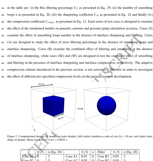
353
relax to a static spherical shape as shown in Fig. 2. It has been shown in the literature [52] that under these
354
conditions and depending on the accuracy of the interface tracking/capturing scheme, non-physical
vortex-355
like velocities may develop in the vicinity of the interface and can result in its destabilization. Tables 1 and 2
356
demonstrate the different controlling parameters that have been tested. The main testing parameters shown
ACCEPTED MANUSCRIPT
in the table are: (i) the flux filtering percentageUf as presented in Eq. 29, (ii) the number of smoothing358
loopsnas presented in Eq. 20, (iii) the sharpening coefficientCshas presented in Eq. 24 and finally (iv)
359
the compression coefficientCcompr.as presented in Eq. 12. Each series of test cases is designed to examine
360
the effect of the mentioned models on parasitic currents and pressure jump calculation accuracy. Cases (S)
361
examine the effect of smoothing loops number in the absence of interface sharpening and filtering. Cases
362
(A) are designed to study the effect of error filtering percentage in the absence of smoothing loops and
363
interface sharpening. Cases (B) examine the combined effect of filtering and smoothing in the absence
364
of interface sharpening, while cases (SE) and (SF) are designed to test the combined effect of smoothing
365
and filtering in the presence of interface sharpening and interface compression, respectively. The adaptive
366
compression scheme introduced in the previous section, is not activated in this case in order to investigate
367
the effect of different pre-specified compression levels on the parasitic current development.
[image:21.595.29.520.88.602.2]368
Figure 2: Computational domain for modelling static droplet, (left) initial condition a cube of sizeD0=30µm, and (right) static
shape of droplet. Mesh size R/δx=15 at t=0.0025 s.
Uf% n(Eq. 20) Uf% n Filter Uf% n(Eq. 20)
Case S1 0 2 Case A1 0.01 0 Case B1 0.05 2
Case S2 0 5 Case A2 0.05 0 Case B2 0.05 5
Case S3 0 10 Case A3 0.1 0 Case B3 0.05 10
[image:21.595.85.474.267.513.2]Case S4 0 20 Case A4 0.2 0 Case B4 0.05 20
Table 1:Case set-up testing the influence of smoothing and capillary filtering values (Uf% andn) without the effect of sharpening or compression coefficients (CshandCcompare set to zero)
The maximum velocity magnitude in the computational domain is presented as a function of various
369
numerical parameters. If inertial and viscous terms balance in the momentum equation then parasitic
ACCEPTED MANUSCRIPT
Uf% n(Eq. 20) Csh(Eq. 24) CcompCase SE1 0.05 10 0.1 0
Case SE2 0.05 10 0.5 0
Case SE3 0.05 5 0.1 0
Case SE4 0.05 5 0.5 0
Case SF1 0.05 10 0.5 0.5
Case SF2 0.05 10 0.5 1
Case SF3 0.05 10 0.5 2
Case SF4 0.05 10 0.5 3
Table 2:Case set-up testing the influence of smoothing and capillary filtering values (Uf% andn) including the effect of sharpening or compression coefficients
ities should be zero. However, the CSF technique introduces an unbalance by replacing the surface force by
371
a volume force which acts over the small region surrounding the continuous phase interface. The surface
372
force suggested by Brackbill et al. [8] includes a density correction as 1/(We ρ
hρiκn) for modelling systems
373
where the phases have unequal density, whereρis the local density andhρiis the average non-dimensional
374
density of the two phases. Including these two variables does not affect the total magnitude of force applied,
375
but weights the force more towards regions of higher density. This tends to produce more uniform fluid
ac-376
celerations across the width of the interface region. Such a force is irrotational and so it can be represented
377
as the gradient of a scalar field. Referring to the momentum equation 2 the surface tension force has to
378
be precisely balanced by the pressure gradient term, with all velocity dependent terms, and thus velocities,
379
being zero. The commonly used VoF numerical implementation of this system differs from this ideal
im-380
plementation ofα, which when discretised represents the volume fraction integrated over the dimensions 381
of a computational mesh cell and varies by a small amount in the radial direction. This results inn-(the
382
normal to the interface) not being precisely directed in the radial direction,κvalue varying slightly and the
383
complete interface volume force having a rotational component. The rotational component of the surface
384
tension force cannot be balanced by the irrotational pressure gradient term. So it must be balanced instead
385
by one or more of the three other velocity dependent terms. As these velocity terms (inertial transient,
in-386
ertial advection and viscous) all require non-zero velocities if they themselves are to be non-zero, spurious
387
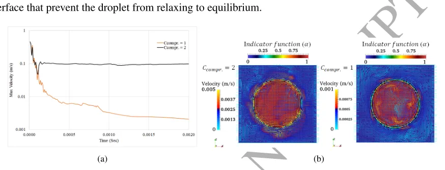
currents develop. Looking into the parasitic velocity magnitude for the standard (interFoam) solver during
388
the relaxation period (Fig. 3a), parasitic velocities are high and depend on the compression level. As the
389
value ofCcompr.increases, the maximum velocity also increases. This might appear to be counter intuitive
ACCEPTED MANUSCRIPT
since increased compression should result in sharper interfaces, nevertheless, in this work the smoothαfield391
is only used for accurate curvature calculation, but for the rest of the equations the sharpened field had been
392
used curvatureκand the normal vectors. However the sharper the interface the more numerical challenging
393
becomes the calculation of derivatives. Fig. 3a indicates this paradox while Figure 3b presents a graphical
394
explanation. It can be seen that asCcompr.increases then vortex like structures develop randomly around the
395
interface that prevent the droplet from relaxing to equilibrium.
396
(a) (b)
Figure 3: (a)Evolution of maximum velocity during droplet relaxation using the standard (interFoam) solver with two different interface compression (Ccompr.).(b) values Snapshot of the interface shape after the relaxation of the oil droplet using the standard
(interFoam). Velocity vectors near to the interface for different interface compression values are presented.
Testing the smoothing effect presented in Eqs. (19, 20 and 21) using the modified solver by varying
397
the number of smoothing loops (n) as shown of Table (1) is also performed in the presented sub-section.
398
The mentioned set-up in cases S1,S2,S3,S4 is used to investigate the effect of smoothing loops on the
399
parasitic currents, isolated from the other examined controlling parameters. It is evident from Fig. 4e that
400
by increasing the number of smoothing loops, the magnitude of the parasitic currents decreases. However,
401
it should be pointed out that this reduction of parasitic currents, comes at the cost of a corresponding
402
increase in the interface region thickness. Increasing the smoothing loops to 20, the interface thickness
403
increases almost 4 times (6 cells) and parasitic currents tend to develop again and increase by time at a
404
certain point after the relaxation of the droplet. The effect of varying the coefficient Uf for filtering the
405
capillary forces parallel to the interface (see Eq. 30) is revealed from cases A1 to A4 of Table 1; a decrease
406
of the parasitic currents due to the wrong flux filtering near to the interface can be noticed. In the absence
407
of smoothing loops and just changing the filter valueUf, a significant decrease of the parasitic currents
408
is observed as shown in Fig. 4b. Moreover, an optimum decrease in parasitic currents using a value of
[image:23.595.67.504.215.382.2]ACCEPTED MANUSCRIPT
Uf =0.05 is observed (Table 1). The decrease of parasitic currents magnitude in this case is a combination410
of the interface treatment of Eq. 19 and the flux filtering without any smoothing loops being performed.
411
Looking at Fig. 4b one can observe the asymmetric distribution of the velocity vector field with almost
412
zero velocity inside the droplet. By examining the isolated filtering coefficientUf and smoothing loops 413
n, the suggested framework has been noticed to reduce the spurious velocities, by almost four orders of
414
magnitude, over a relatively long period. Cases B1 to B3 of Table 1 reveal the effect of combining both
415
techniques (smoothing and flux filtering) for damping the parasitic currents; one of the parameters has kept
416
constant - in this case,Uf. Comparing cases (B2) presented in Figures 4c with the previously presented
417
cases S and A, a major improvement in velocity reduction can be seen. In Fig 5 (B) a reduction of almost
418
four orders of magnitude, when compared with the standard solver, has been achieved. By examining the
419
deviation from the theoretical results compared to the standard interFoam using filtering and smoothing
420
models as shown in Table 3, the suggested models reduce the maximum velocity field as seen in cases (S2
421
and A1), then it start to increase, due to the excessive interface smoothing or the un-balanced capillary
422
forces. Selecting the best smoothing and the filtering coefficient combination ( 5<n<10 andUf =0.05),
423
the effect of the sharpening model Eq. 24 is now examined. In Table 2 cases (SE1 to SE4), theCshhas
424
been varied. Looking at Fig. 4a, a great reduction in the interface thickness can be seen reaching almost
425
one grid cell. By combining the effect of sharpening, filtering and smoothing techniques, the same order
426
of magnitude for parasitic currents with a significant decrease in interface thickness has been achieved. It
427
has also been found that in SF1 case specifically, a very good balance in the velocity vector field with zero
428
velocity inside the droplet (Fig. 5) has been achieved.
429
As mentioned before, the literature review has revealed the negative effect of increasing the value of
430
compression coefficient, since as the value ofCcompr. increases the magnitude of parasitic currents also
431
increases. Using the same droplet test case, the effect of increasing theCcompr.value on the parasitic current
432
is demonstrated, but this time after applying the smoothing and flux filter models. It should be noted, the
433
aforementioned adaptive compression model is not tested in this case yet, as it will be tested in the next
434
section. In Table 2 cases (SF1 to SF4), the cases using the best combination of the previously mentioned
435
smoothing and filter values coefficient are used with different compression values. The overall maximum
436
velocity values are higher compared to those archived using no compression;nevertheless, these are still
ACCEPTED MANUSCRIPT
(a) SF1 (b) A2
(c) B2 (d) SE4 (e) S3
Figure 4: Effect of varying model coefficients described in table 1 and 2 on parasitic currents, all figures are showing velocity vector field at t=0.0024 sec. Figures are coloured with indicator functionαS harpas yellow showing oil phase inside the droplet and
bright blue showing water outside the droplet
lower than those achieved using the standard solver. A swirling behaviour around the external diagonal
438
direction of the droplet had been noticed as shown in Fig. 4b and 4c. The observed small swirling velocity
439
confirms that the unbalanced surface tension force may increase parasitic currents at one specific location
440
due to this swirling behaviour around the droplet interface. At the same time the effects of the smoothing
441
and the filtering can have positive effect on decaying these swirling velocities.
442
The behaviour of the droplet when different parameters are considered is important in assessing the
443
impact that the parasitic currents have on the results. Similar simulations but with varying domain sizes
444
(not included in this study) showed that when the parasitic currents were inertia-driven at the deformation
445
phase they spread further across the computational domain. Depending on the nature of the simulation
446
being considered, this may mean that inertia-driven parasitic currents have a greater impact on the results.
447
Quantifying this effect would be difficult, as any integral measure of the parasitic currents – such as the
448
total kinetic energy within the domain for example – would be dependent on additional geometrical factors,
449
such as the domain size and interfacial area. While the form of the velocity field is changing with time
[image:25.595.73.502.105.371.2]ACCEPTED MANUSCRIPT
Figure 5: Effect of varying models coefficients presented in table 1 and 2 on maximum parasitic currents over period of timeone can conclude that the parasitic currents are dominated by inertia. The assessment of the effect of
451
different parameters on the maximum velocity can also be presented in the percentage of divergence from
452
the standard solver results as illustrated by Eq. 31;
453
Eparasitic= min(U)min(U) Cα=2
(31)
whereEparasiticrepresents the error calculated by themin(U) to be the minimum velocity in the domain
454
achieved using modified solver andmin(U)Cα=2to be minimum velocity using standard solver atCcompr.=2 455
during the droplet relaxation over a long time interval. Table 3 shows that the magnitude of parasitic currents
456
decreases to minimal in case (B2) where compression and sharpening are null; one can also achieve the same
457
level of reduction in parasitic currents after applying sharpening, as in case (SE3) and with only a slight
458
further increase by adding compression as in case (SF1). Table 3 shows numerically predicted pressure
459
difference between the relaxed spherical droplet and the ambient liquid along the droplet diameter axis for
460
each of the 20 simulated cases, in comparison with the theoretical value predicted from the Laplace equation
461
[see [53] for more details]. The results are presented in terms of the errors in predicted capillary pressure,
462
ErrorPc, defined as follows:
463
Errorpc =
pc−(pc)theoretical (pc)theoretical /
P−Ptheoretical Ptheoretical
ACCEPTED MANUSCRIPT
wherepcis the calculated capillary pressure using the developed solver, and thePis the calculated pressure 464using the standard interFoam with compression value of two. TheErrorpcpresents the deviation of the
cal-465
culated capillary pressure using the developed solver and the standard solver with respect to the theoretical
466
capillary pressure. Equation 32 shows the reduction in error between the developed solver and the standard
467
solver using compression (Ccompr. = 2). In all the presented cases, reduction in predicting the capillary
468
pressure by 40% can be seen.
469
S mooth S1 S2 S3 S4
Errorpc% 41.43 40.57 39.64 33.38
Eparasitic 0.0051 0.0053 0.0080 0.0112
Filter A1 A2 A3 A4
Errorpc% 45.55 45.51 45.51 45.63
Eparasitic 0.0031 0.0006 0.0011 0.0014
Filter B1 B2 B3 B4
Errorpc% 44.36 43.39 42.20 40.91
Eparasitic 0.0005 0.0006 0.0013 0.0032
S harp S E1 S E2 S E3 S E4
Errorpc% 43.04 45.14 43.97 46.11
Eparasitic 0.0008 0.0024 0.0007 0.0015
S harp S F1 S F2 S F3 S F4
Errorpc% 49.79 50.20 50.12 49.95
Eparasitic 0.0008 0.0045 0.0057 0.0067
Table 3: Reduction in predicted capillary pressure and parasitic currents compared to the standard interFoam
4.2. Interacting Parasitic Currents of two relaxing droplets
470
In this section the effect of parasitic current interaction for the case of two stagnant droplets that undergo
471
the same relaxation process is discussed. The same droplet properties as in the previous test case have been
472
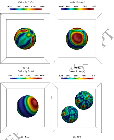
used (see Section 4.1). When two droplets are found in the same domain in close proximity, the parasitic
473
currents may interact resulting in artificial movement of the droplets and eventually merging. Figure 7
474
shows the velocity magnitude on the droplet represented by the 0.5 liquid volume fraction iso-surface. The
475
same set of parameters are utilised as in (A2, B2, SE3 and SF1) cases mentioned in Tables 1 and 2. One
476
can notice in Fig. 7a to Fig. 7c that the two droplets have merged to one big droplet located at the centre of
ACCEPTED MANUSCRIPT
Figure 6: Computational domain showing two static droplets , (left) initial condition a cube of sizeD0=20µm each, and (right)static shape of droplet as two boxes.
the computational domain. In contrast Fig. 7d shows that the two droplets remain in their initial position as
478
they should. This can be considered as a demonstration that optimising compression for one case does not
479
necessarily mean that can offer optimum results for other similar cases and the solver should automatically
480
adapt the needed compression. Hence, in the next sections that consider cases with higher deformation of
481
the interface we are going to introduce the adaptive solver.
482
4.3. Notched disc in rotating flow
483
In addition to the static droplet test cases, the rotation test of the slotted disk, which is known as the
484
Zalesak problem [51] has been tested. The Zalesaks circle disk is initially slotted at the centre (0.5,0,0.75) of
485
a 2D unit square domain. The disk is subjected to a rotational movement under the influence of a rotational
486
field that is defined by the following equations:
487
u(x)=−2π(x−x0) (33)
w(z)=2π(z−z0) (34)
where u(x), w(z) are the imposed velocity components. By applying this velocity, one complete rotation
488
of the disk is completed within t=1sec. For all simulations performed for this test case, a fixed time-step has
489
been used, keeping the Courant number equal to 0.5. The initial disk configuration used for the simulation
ACCEPTED MANUSCRIPT
(a) A2 (b) B2
(c) SE3 (d) SF1
Figure 7: Effect of combined flux filtering and smoothing in the presence of sharpening model on the interaction of parasitic velocity field. All figures are showing the velocity field at t=0.0024 sec on the indicator functionαS harpiso-contour=0.5
is presented in Fig. 8. Three different mesh densities were used consisting of 64x64, 200x200 and 400x400
491
cells, respectively.
492
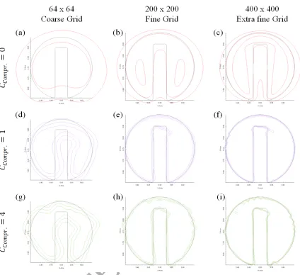
Figures 9 and 10 show the comparison between the standard solver using different compression (Ccompr.)
493
values and the developed adaptive solver using different sharpening (Csh) values. In each plot, the exact
494
initial and final interface shape is presented. In all the figures, the iso-contours values of indicator function
495
alpha αof (0.1, 0.5 and 0.9) after one revolution of the disk are shown. The reason of presenting three
[image:29.595.121.487.105.551.2]ACCEPTED MANUSCRIPT
Figure 8: Schematic representation of two dimensional Zalesak’s Disk benchmark test case described at [54].contour lines is to better explore the effect of the adaptive compression model on both the interface diffusion
497
and the overall disk shape. For the coarse mesh (64x64) neither using the standard interFoam with three
498
compression values (Ccompr. =0, 1 and 4)), nor the three values forCsh, (Csh = 0.1, 0.5 and 0.9) for the
499
adaptive modified solver, can provide a satisfactory interface representation. One can even notice that due
500
to the large interface deformation and diffusion, the interface iso-contour of α = 0.9 at Fig. 9(a) has
501
disappeared for the standard solver. Nevertheless, for the adaptive modified solver cases, the modified
502
solver can keep the main geometrical features as seen in Figs. 10(a,d,g). By using high compression as
503
in Fig. 9(g) , one can notice a reduction in the interface thickness, although a rather high deformation
504
and corrugated shape of the final disk shape has been noticed. Comparing Fig. 9(g) to Fig. 10(g) one
505
can notice the effectiveness of the adaptive model that preserves the geometrical outline of the disk while
506
the sharpening model decreases the interface thickness. Moving to a finer mesh (200x200), high interface
507
diffusion using the standard interFoam with no compression (Ccompr.=0) Fig. 9(b) has been noticed. The
508
higher grid resolution is not adequate to provide remedies to the previously mentioned deficiencies noticed
509
in the coarser mesh using interFoam. The highly diffusive interface using the standard interFoam also did
510
not maintain the 0.9 iso-contour making two oval shapes at the sides. For higher compression values Fig.
511
9(e,h) although the disk shape is preserved by the standard solver, the interface is significantly deformed
512
near the outer disk boundary. Use of the adaptive solver Fig. 10(b,e,h) shows better consistency for the shape
513
regardless of the imposed sharpening level. Moreover, the adaptive compression eliminates any irregular
ACCEPTED MANUSCRIPT
Figure 9: Zalesak disk after one revolution. Iso-contours for indicator function alpha (α=0.1, 0.5 and 0.9) are plotted for the standard interFoam using different compression values, together with the reference shape.shapes compared to the standers solver. Figure 10(h) especially shows an excellent agreement with the
515
original circular shape layout. This test case also demonstrates the role of the sharpening valueCshwhich
516
can help in controlling the interface diffusion depending on the case under consideration. To examine our
517
adaptive solver mesh dependency, the mesh has been doubled to 400x400. Even for this fine grid resolution
518
case the standard solver gives inaccurate disk shape regardless of the compression value used, as none of
519
them is adequate to balance the interface shape. A zero compression value using the standard interFoam
520
preserves the characteristic shape for the first time (see Fig. 9(c), compared to Fig. 9(a,b)). For the higher
521
compression values as in Fig. 9(f,i), high corrugated regions at the interface have been observed. Using the