MVDR broadband beamforming using polynomial matrix techniques

MVDR BROADBAND BEAMFORMING USING POLYNOMIAL MATRIX TECHNIQUES

S. Weiss

, S. Bendoukha

, A. Alzin

, F.K. Coutts

, I.K. Proudler

, J. Chambers

1

_{Department of Electronic & Electrical Engineering, University of Strathclyde, Glasgow, Scotland}

_{Department of Electrical Engineering, College of Engineering, Taibah University, Yanbu, Saudi Arabia}

3

_{School of Electrical, Electronics & Systems Engineering, Loughborough Univ., Loughborough, UK}

_{School of Electrical and Electronic Engineering, Newcastle University, Newcastle upon Tyne, UK}

ABSTRACT

This paper presents initial progress on formulating minimum variance distortionless response (MVDR) broadband beam-forming using a generalised sidelobe canceller (GSC) in the context of polynomial matrix techniques. The quiescent vec-tor is defined as a broadband steering vecvec-tor, and we propose a blocking matrix design obtained by paraunitary matrix com-pletion. The polynomial approach decouples the spatial and temporal orders of the filters in the blocking matrix, and de-couples the adaptive filter order from the construction of the blocking matrix. For off-broadside constraints the polynomial approach is simple, and more accurate and considerably less costly than a standard time domain broadband GSC.

1. INTRODUCTION

If broadband signals need to be resolved by an array, sen-sor elements usually have to be followed by tap delay lines in order to capture the relative lag rather than just a phase shift between signals. This has led to the extension of many narrowband beamforming techniques to the broadband case, such as minimum variance distortionless response and one of its realisations, the generalised sidelobe canceller [1].

To describe broadband array signals and MIMO systems, covariance and transfer functions can be denoted as polyno-mial matrices [2]. For such quantities, narrowband techniques such as EVD and SVD have been extended to polynomials, with applications in denoising-type [3] or decorrelating pre-processors [4], transmit and receive beamforming across broadband MIMO channels [5, 6], broadband angle of ar-rival estimation [7], and for optimum subband partitioning of beamformers [8].

Here, polynomial matrix techniques are extended to the MVDR problem. We will demonstrate below that this can provide an elegant framework particulary when designing beamformers with arbitrary look direction. Most beam-former designs assume presteering and look towards

broad-This work was supported in parts by the Engineering and Physical Sciences Research Council (EPSRC) Grant number EP/K014307/1 and the MOD University Defence Research Collaboration in Signal Processing.

side [9–11], where the constraint can be inexpensively imple-mented [12]. This work complements the sparse literature on designs with an arbitary look direction [13], with a significant reduction in complexity.

2. MVDR BEAMFORMING

This section briefly reviews narrowband MVDR beamform-ing in Sec. 2.1 and comments on its standard extension to the broadband case in Sec. 2.2.

2.1. MVDR and Generalised Sidelobe Canceller

Ifx[n]∈CM is a vector of sensor signals with space-time co-varianceR[τ] =Ex[n]xH[n−τ], ande[n] =wHx[n]the output of a beamformer with coefficients inw, then the nar-rowband MVDR beamformer optimises the constrained prob-lem

min

w E

|e[n]|2_{= min}

w w

H_{R[0]w (1)}

s.t. sH(ϑ_s,Ω)w= 1, (2)

whereby the constraint by a steering vectorsH(ϑs,Ω) pro-tects the signal of interest in look directionϑsat normalised angular frequencyΩ.

Instead of solving the MVDR problem directly, a GSC forms a quiescent beamformerwq which points in direction

ϑs and minimises (1) for spatially white noise. Its output

d[n] =wH

qx[n]in general still contains interference. There-fore, a blocking matrixB, whose rows span the nullspace of

wqsuch thatBwq = 0, can generate a signalu[n] =Bx[n] containing interference only. In an unconstrained optimisa-tion step, a noise cancelling filterwacan therefore be applied such thate[n] = d[n]−wH_au[n]contains no more interfer-ence, enforcingE{u[n]e∗[n]}= 0.

2.2. Broadband Case

˜

wq(z)

B(z) w˜a(z) ₋+

d[n]

e[n]

y[n]

x[n]

u[n]

Fig. 1. Generalised sidelobe canceller with polynomial

qui-escent vector and polynomial blocking matrix; the system wa(z)represents a multichannel adaptive filter.

that e.g.x ∈ CML. While this is generally straightforward, we here focus on the formulation of constraints. A constraint matrixCcontains columns of steering vectors in direction of

ϑsover a set of frequencies,

C= [s(ϑs,Ω0), s(ϑs,Ω1) . . . s(ϑs,ΩL−1)] (3)

and the constraint equationCHw=fdefines the desired fre-quency response inf ∈CLfor look directionϑs. For a planar array, the simplest constraint is towards broadside, whereC is assembled fromLidentity matrices, but in principle, the

Lpoint constraints defined via (3) can also be applied for an off-broadside look direction [13].

3. PROPOSED APPROACH 3.1. Polynomial MVDR and GSC

Definingw(z)∈CM to contain the complex conjugated and time-reversed M beamforming filters and R(z)•—◦R[τ] as thez-transform of space-time covariance matrix, the out-put power spectral density of the beamformer is Re(z) =

˜

w(z)R(z)w(z)leads to the MVDR problem formulation

min

w(z)

|z|=1Re(z)

dz

z (4)

s.t. ˜s(ϑ_s, z)w(z) =F(z), (5)

with the parahermitian transpose operationw˜(z) =wH(z−1). The broadband steering vectors(ϑs, z)defines the look di-rection of the array with a desired frequency responseF(z). For simplicityF(z) = 1is assumed.

To solve (4) and (5), we propose the polynomial GSC shown in Fig. 1. The quiescent beamformerw_q(z)is derived from the constraint (5), which in turn defines a blocking ma-trixB(z)and a multichannel adaptive filter with coefficients inw_a(z). Below, these components are elaborated in turn.

3.2. Broadband Steering Vector and Quiescent Beam-former

A broadband steering vectors(ϑ, z)contains explicit delays rather than phase shifts as in the narrowband case, such that

0 0.05 0.1 0.15 0.2 0.25 0.3 0.35 0.4 0.45 0.5

−80 −70 −60 −50 −40 −30 −20 −10 0

normalised angular frequencyΩ/(2π)

20

lo

g10

|

E1

(

e

j

Ω)|

T=50 T=100

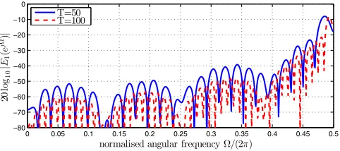
Fig. 2. ErrorE2(z) = ˜s(30◦, z)s(30◦, z)−1 evaluated on

the unit circle, with windowed sinc functions of orderT as fractional delay filters.

sϑ[n]◦—•s(ϑ, z)

sϑ[n] = √1

M

⎡ ⎢ ⎢ ⎢ ⎣

d[n] d[n−τ2(ϑ)]

.. .

d[n−τM(ϑ)]

⎤ ⎥ ⎥ ⎥

⎦, (6)

whered[n−τ]is an ideal fractional delay byτ ∈ R sam-ples. A waveform from directionϑexperiences a lagτm(ϑ) relative to elementm = 1when it arrives at themth sensor. Evaluating (6) at frequencyΩturns the delaysd[n−τm(ϑ)] into phase shifts ands_ϑ[n]into a narrowband steering vector as discussed in Sec. 2.1. With (6),˜s(ϑ, z)s(ϑ, z) = 1is easily verified.

To implement a broadband steering vector according to (6) requires fractional delay filters. With relatively moder-ate order, high accuracy can be achieved close up to half of the sampling rate using e.g. windowed sinc functions [14,15]. An example for the accuracy ofs(ϑ, z)withϑ= 30◦for a linear, critically sampled array withM = 8equispaced elements is shown in Fig. 2.

Assuming that˜s(ϑ, z)s(ϑ, z)≈1for the steering vectors constructed above, forF(z) = 1(5) is fulfilled withw_q(z) = s(ϑs, z). Therefore, the output of the quiescent beamformer is

d[n] =T

ν=0

wH

q[−ν]x[n−ν]. (7)

Note thatw_q(z)•—◦w_q[n]is of orderTand holds the para-hermitian transpose of the actual coefficients.

3.3. Blocking Matrix

The blocking matrix has to be designed such that

B(z)wq(z) = 0 . (8)

To achieve orthonormality betweenB(z)andw_q(z), a pa-raunitary matrix

can be constructed with Q(z) ˜Q(z) = I and B˜(z) = BH(z−1_{). For the narrowband or standard broadband cases} using matrices and vectors with scalar entries, this can be achieved by a variety of methods such as singular value decomposition of the constraint vector/matrix, or orthogo-nalisation of the columns in (9) using Gram-Schmidt or QR decompositions [16]. However, the polynomial case is more involved and will be separately addressed in Sec. 4.

The output of the blocking matrix, u[n] ∈ CM−1 as shown in Fig. 1, is

u[n] =N

ν=0

B[ν]x[n−ν], (10)

whereB[n]◦—•B(z)is of orderN. This orderN impacts on the computational complexity ofB(z)and will arise from its construction in Sec. 4.

3.4. Multichannel Noise Cancellation

Withw_q(z)andB(z)as defined previously, a multichannel filterw_a(z)∈CM−1can be employed to remove the remain-ing interference from the quiescent beamformer outputd[n] usingu[n], as shown in Fig. 1. Withw_a(z)containing the parahermitian of the actual filter coefficients, the beamformer output is

e[n] =d[n]−L ν=0

wH

a[−ν]u[n−ν], (11)

wherebyw_a[n]◦—•w_a(z)is of orderL.

The multichannel filterwa(z)can be determined through unconstrained minimisation ofE|e[n]|2. Various tools ex-ist, such as MMSE or Wiener solution, as well as adaptive techniques such as LMS or RLS [17]. For simulations in Sec. 6, the multichannel normalised LMS (NLMS) algorithm will be used.

4. PARAUNITARY MATRIX COMPLETION This section proposes a paraunitary matrix completion to find aQ(z)in (9) based onw_q(z). For this, we employ a polyno-mial eigenvalue decomposition (PEVD, [18]) of the rank one matrix

wq(z) ˜wq(z) = ¯Q(z)D(z) ˜¯Q(z). (12)

The PEVD approximately diagonalises and spectrally ma-jorisesD(z)by means of a paraunitary matrixQ¯(z). Spectral majorisation is equivalent to ordering in the SVD [16], and ensures that the energy is compacted into as few polynomial eigenvalues inD(z)as possible. Sincewq(z)has unit norm and (12) is rank one by construction, we obtain

D(z) =diag{1 0 . . . 0}. (13)

0 0.05 0.1 0.15 0.2 0.25 0.3 0.35 0.4 0.45 0.5

−55 −50 −45 −40 −35 −30 −25

normalised angular frequencyΩ/(2π)

20

lo

g10

|

E2

(

e

j

Ω)|

truncation 1e-4,N= 164

truncation 1e-3,N= 140

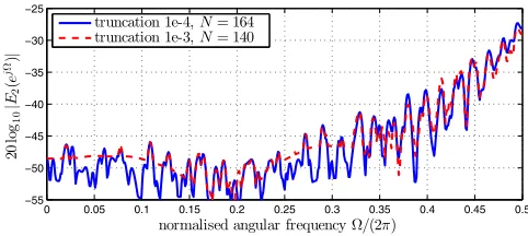
Fig. 3. Leakage of blocking matrix according to (17).

The paraunitary matrix Q¯(z) is ambiguous even if (12) had full rank. If

¯

Q(z) = [¯q₁(z) ¯q₂(z) . . . q¯M(z)], (14)

thenq¯₁(z)could e.g. be a shifted version of the polynomial vectorswq(z),

¯

q₁(z) =z−Δwq(z), (15)

and still satisfy both (12) and (13). Similarly, the remaining columnsq¯_m(z)could be arbitrarily shifted. Therefore, when defining

˜

B(z) = [¯q₂(z) . . . q¯_M(z)], (16)

˜

B(z)wq(z) = 0is guaranteed, butB(z)may have a larger order than necessary. Through appropriate shift of rows and truncation of small outer coefficients ofB(z)[19], this order can be reduced.

Example. Using the previous example of wq(z) = s(30◦_{, z)with T = 50 and the above procedure, B(z) is}

calculated by sequential matrix diagonalisation [20], which implements an iterative PEVD algorithm. To measure how much of the signal of interest leaks through the blocking ma-trix — which can result in signal cancellation in the GSC — the following error metric defined over a set of frequencies

{Ωi},

E2(ejΩi) = max m∈{2...M}|¯q

H

m(e−jΩi)wq(ejΩi)| (17)

extracts the maximum error across allM−1inner products at every frequency. The result for truncation ofB(z)by 1‰ and 0.1‰ of its energy is shown in Fig. 3. The error is acceptable particularly at low frequencies. It is dominated by inaccura-cies in the construction of the broadband steering vector, but not by the iterative PEVD or the truncation ofB(z).

5. PERFORMANCE METRICS

Table 1. Computational complexity of different broadband beamformer realisations in multiply accumulates (MACs).

GSC cost

component polynomial standard quiescent beamformer M(T+1) M(L+1)

blocking matrix M(M−1)(N+1) M(M−1)(L+1)2

adaptive filter (NLMS) 2(M−1)(L+1) 2(M−1)(L+1)

by the broadband steering vectors(ϑ, z), the overall transfer function of the source and beamformer is

A(ϑ, z) = ( ˜wq(z)−w˜a(z)B(z))·s(ϑ, z). (18)

The directivity pattern is the magnitude of the response

A(ϑ, ejΩ_{), which is obtained by probing (18) with a series of} steering vectors and evaluating it on the unit circle.

Residual Error. To assess convergence of the optimisation methods for wa(z), a useful metric is to assess the mean square of the residual errorer[n], obtained by subtracting the source signal projected through the quiescent vector from the errore[n].

Computational Cost. The computational complexity of the various polynomial GSC components in Sec. 3 is listed in Ta-ble 1. For comparison, the costs for a time domain broad-band beamformer is also stated [12]. An off-broadside look direction can be enforced through point constraints in the fre-quency domain, but prevents simplifications to the blocking matrix, which has to be applied to the full spatio-temporal data vector of dimensionM L.

6. SIMULATIONS AND RESULTS

We assume a signal of interest fromϑ= 30◦, and three in-terferers from anglesϑi∈ {−40◦,−10◦,80◦}active over the frequency rangeΩ = 2π·[0.1; 0.45]at signal to interference ratio of -40 dB. TheM = 8element linear uniform array is also corrupted by spatially and temporally white additive Gaussian noise at 20 dB SNR.

An example for the directivity pattern of wq(z) = s(30◦_{, z)withT = 50, is shown in Fig. 4. A time domain}

broadband quiescent beamformer designed fromT+ 1point constraints in the frequency domain is provided as a bench-mark in Fig. 5. Both beamformers are similar, but while the polynomial version has inaccuracies in look direction towards

Ω = πdue to the broadband steering vectors lacking preci-sion, the standard approach has inaccuracies particularly at the lower end of the spectrum, as will be seen later in Fig. 9.

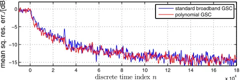
With a quiescent design ofT = 50as shown previously and a blocking matrix via PEVD completion with orderN = 140, an L = 175order NLMS algorithm optimiseswa(z). The convergence curve is shown in Fig. 6, together with that of a standard time domain broadband GSC of same dimen-sionL. The directivity patterns with convergedw_a(z)are

angle of arrivalϑ/[◦]

20

lo

g10

|

A

(

ϑ,

e

j

Ω)

|

/[

d

B

]

Ω 2π

Fig. 4. Directivity pattern of polynomial quiescent

beam-former with look directionϑs= 30◦.

angle of arrivalϑ/[◦]

20

lo

g10

|

A

(

ϑ,

e

j

Ω)|

/[

d

B

]

Ω 2π

Fig. 5. Directivity pattern of standard broadband quiescent

beamformer with look directionϑs= 30◦.

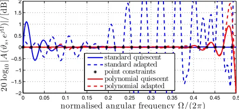
in Fig. 7 for the proposed polynomial approach and Fig. 8 for the benchmark. Both beamformers have placed nulls to-wards the three interferers, but the polynomial approach pro-tects the constraint better — an example for the gain in look direction, which is constrained to 0 dB, is shown in Fig. 9 for

T =L= 50before and after adaptation. While the standard approach oscillates strongly between its point constraints, the polynomial approach is much better behaved.

With the above parameters and the cost as listed in Ta-ble 1, the proposed beamformer requires 10.7 kMACs, while the standard broadband beamformer takes almostLtimes as much with 1.72 MMACs per iteration step.

0 2 4 6 8 10 12 14 16 18

x 104

−15 −10 −5 0

mean sq. res. err./[dB]

discrete time indexn

standard broadband GSC polynomial GSC

Fig. 6. Mean square residual error for proposed polynomial

angle of arrivalϑ/[◦]

20

lo

g10

|

A

(

ϑ,

e

j

Ω)

|

/[

d

B

]

Ω 2π

Fig. 7. Directivity pattern of adapted polynomial GSC.

angle of arrivalϑ/[◦]

20

lo

g10

|

A

(

ϑ,

e

j

Ω)|

/[

d

B

]

Ω 2π

Fig. 8. Directivity pattern of adapted standard GSC.

7. CONCLUSIONS

A polynomial matrix formulation of a GSC implementing an MVDR beamformer has been introduced, which requires the definition of constraints via broadband steering vectors. For the construction of the blocking matrix, a paraunitary matrix completion has been defined. The proposed method can el-egantly and compactly handle off-broadside constraints and define metrics such as the directivity pattern, and can lead to accurate beamformers of considerably lower complexity compared to the standard time domain counterpart.

REFERENCES

[1] B.D. Van Veen and K.M. Buckley, “Beamforming: a versatile approach to spatial filtering,” IEEE ASSP Mag., 5(2):4–24, Apr. 1988.

[2] P.P. Vaidyanathan, Multirate systems and filter banks, Pren-tice Hall, 1993.

[3] S. Redif, J.G. McWhirter, P.D. Baxter, and T. Cooper, “Ro-bust broadband adaptive beamforming via polynomial eigen-values,” inOCEANS, Boston, MA, Sep. 2006, pp. 1–6. [4] C.L. Koh, S. Redif, and S. Weiss, “Broadband GSC

beam-former with spatial and temporal decorrelation,” in EU-SIPCO, Glasgow, UK, Aug. 2009, pp. 889–893.

[5] M. Davies, S. Lambotharan, and J.G. McWhirter, “Broadband MIMO beamforming using spatial-temporal filters and poly-nomial matrix decomposition,” inInt. Conf. DSP, Cardiff, UK, July 2007, pp. 579–582.

0 0.05 0.1 0.15 0.2 0.25 0.3 0.35 0.4 0.45 0.5

−2 −1.5 −1 −0.5 0 0.5 1 1.5 2

normalised angular frequencyΩ/(2π)

20

lo

g10

|

A

(

ϑs

,e

j

Ω)|

/[

dB]

standard quiescent standard adapted point constraints polynomial quiescent polynomial adapted

Fig. 9. Gain in look directionϑs= 30◦before and after

adap-tation.

[6] C.H. Ta and S. Weiss, “A design of precoding and equalisation for broadband MIMO systems,” inInt Conf. DSP, Cardiff, UK, July 2007, pp. 571–574.

[7] M. Alrmah, S. Weiss, and S. Lambotharan, “An extension of the MUSIC algorithm to broadband scenarios using poly-nomial eigenvalue decomposition,” inEUSIPCO, Barcelona, Spain, Aug. 2011, pp. 629–633.

[8] P.G. Vouras and T.D. Tran, “Robust transmit nulling in wide-band arrays,”IEEE Trans. SP,62(14):3706–3719, July 2014. [9] I. Thng, A. Cantoni, and Y.H. Leung, “Derivative constrained optimum broad-band antenna arrays,” IEEE Trans. SP, 41(7):2376–2388, July 1993.

[10] S. Zhang and I.L.-J. Thng, “Robust presteering derivative constraints for broadband antenna arrays,” IEEE Trans. SP, 50(1):1–10, Jan. 2002.

[11] M. R¨ubsamen and A.B. Gershman, “Robust presteered broad-band beamforming based on worst-case performance opti-mization,” in5th IEEE SAM, Darmstadt, Germany, July 2008, pp. 340–344.

[12] W. Liu and S. Weiss, Wideband Beamforming — Concepts and Techniques, Wiley, 2010.

[13] M.R. Sayyah Jahromi and L.C. Godara, “Steering broad-band beamforming without pre-steering,” in IEEE/ACES Int. Conf. Wireless Comms & Applied Comp. Electromag., Apr. 2005, pp. 987–990.

[14] J. Selva, “An efficient structure for the design of variable frac-tional delay filters based on the windowing method,” IEEE Trans. SP,56(8):3770–3775, Aug. 2008.

[15] M.A. Alrmah, S. Weiss, and J.G. McWhirter, “Implemen-tation of accurate broadband steering vectors for broadband angle of arrival estimation,” inIET Intelligent Signal Proc., London, UK, Dec. 2013.

[16] G.H. Golub and C.F. Van Loan, Matrix Computations, John Hopkins, 1996.

[17] S. Haykin,Adaptive Filter Theory, Prentice Hall, 1991. [18] J.G. McWhirter, P.D. Baxter, T. Cooper, S. Redif, and J.

Fos-ter, “An EVD Algorithm for Para-Hermitian Polynomial Ma-trices,”IEEE Trans. SP,55(5):2158–2169, May 2007. [19] J. Corr, K. Thompson, S. Weiss, I.K. Proudler, and

J.G. McWhirter, “Row-shift corrected truncation of parauni-tary matrices for PEVD algorithms,” submitted toEUSIPCO, Nice, France, September 2015.