Analysis of the Technical Performance of
C
2
C Operation for HV Networks
December 2014
Steven Blair, Campbell Booth University of Strathclyde
Abbreviations
C2C Capacity to Customers
CAD Computer Aided Design
CHP Combined Heat and Power
CIM Common Information Model
CPU Central Processing Unit
CSV Comma-Separated Values
DG Distributed Generation
DINIS Distribution Network Information System
DSR Demand-Side Response
ENWL Electricity North West Limited
HV High Voltage (6.6 kV or 11 kV)
IPSA Interactive Power System Analysis
LF Load Factor
LLF Loss Load Factor
LV Low Voltage (typically 400 V)
Ofgem Office of Gas and Electricity Markets
OHL Overhead Line
NOP Normally Open Point
Plt Long Term Flicker
Pst Short Term Flicker
pu Per Unit
PV Photovoltaic
RMS Root Mean Square
RTU Remote Terminal Unit
SD Secure Digital
TDD Total Demand Distortion
THD Total Harmonic Distortion
UTC Coordinated Universal Time
Version History
Version Date Comments
1.0 15th December 2014 First issue
Contents
Chapter 1 : Executive Summary ... 3
Chapter 2 : Introduction ... 5
Chapter 3 : Impact of C2C Operation on Released Demand Capacity ... 7
Chapter 4 : Impact of C2C Operation on Released DG Capacity ... 31
Chapter 5 : Impact of C2C Operation on HV Network Technical Losses ... 49
Chapter 6 : Impact of C2C Operation on Power Quality ... 64
Chapter 7 : Impact of C2C Operation on HV Fault Levels ... 85
Chapter 8 : Key Conclusions and Learning Outcomes ... 98
Appendix A : Electrical System Modelling ... 101
Appendix B : Effects of Modelled DG Power Factor ... 110
Appendix C : Processing Raw Demand Data ... 113
Appendix D : Sensitivity of Losses to Load Type ... 115
Appendix E : Assessment of ENWL Network Data Sources ... 119
Appendix F : Voltage Harmonic Distortion Simulation Parameters ... 123
Appendix G : Power Quality Monitoring Data Import and Validation Process ... 127
Chapter 1: Executive Summary
This report evaluates the technical benefits of the Capacity to Customers (C2C) project, an Ofgem Low Carbon Network Fund project led by Electricity North West Limited (ENWL) in conjunction with several industrial and academic partners.
The objective of the C2C project is to test a combination of new automation technology, non-conventional network operational practices (i.e., increased network interconnection), and commercial demand-side response (DSR) contracts. These changes will allow ENWL to increase interruptible demand and generation connections on a selection of trial circuits without resorting to conventional reinforcement measures. The project will thereby “release” inherent spare capacity in the high voltage (HV) system in order to accommodate the future forecast increases in demand and DG, and will therefore assist in meeting the UK’s ambitious CO2 emission targets.
This report documents work undertaken by the University of Strathclyde to quantify the technical performance of C2C network operation on electrical distribution systems. Specifically, this report analyses the impact of C2C operation on available demand capacity, DG capacity, electrical losses, power quality, and fault levels. This has been achieved using simulation models based upon actual system data and through the analysis of power quality monitoring data gathered from a representative proportion of the C2C trial circuits. The results in this report determine the theoretical maximum limits and effects of C2C operation on the aforementioned criteria. Particular attention is given to quantifying the benefits of interconnected (closed-ring) HV network operation over conventional radial (open-ring) operation.
The simulation studies of actual C2C trial circuits have shown that C2C operation can release significant demand and DG capacity. On average, C2C operation can achieve up to approximately a 76% increase in demand and a 225% increase in DG, compared with defined base case scenarios. However, the results depend significantly on the individual circuit topologies, the thermal ratings of circuit sections, and load or DG locations. On average, Interconnected C2C operation (with closed HV rings) releases more demand and DG capacity when compared to Radial C2C operation (with radial HV feeders). Furthermore, a “holistic” system approach is required when considering the connection of load or generation; other technical factors (such as primary transformer ratings) or non-technical factors (such as cost-effectiveness) may affect the maximum capacity which can be released by a particular HV circuit.
approximately 0.3% higher than the equivalent losses assumed from conventional reinforcement of the radial networks, but this must be offset against benefits accrued in the intervening period between introduction of C2C and the time when the maximum C2C capacity is reached (which would span many years).
Power quality measurements from several locations throughout the ENWL network and spanning a significant period of the duration of the C2C trial have been analysed to compare the effects of Radial C2C operation and Interconnected C2C operation. Extensive validation of the monitoring data has been performed to ensure that the comparisons are sound. C2C operation is likely to have only a marginal impact on power quality. This has been confirmed through theoretical analysis of the likely change in voltage total harmonic distortion (THD) resulting from Interconnected C2C operation. In particular, the measurement data indicate that the worst case mean THD measured at LV, approximately 3%, is well within the planning level of 5%.
Chapter 2: Introduction
2.1 “Capacity to Customers” project overview
Distribution networks must be equipped for a significant increase in future electrical demand, due to the continuing electrification of transport and heating to meet the UK’s ambitious CO2 emission targets [1]. Furthermore, the proliferation of distributed generation (DG) can sometimes be inhibited by lack of available network capacity. The challenges associated with these developments must be met in a cost-effective manner and without undue environmental impact. It is also important that future capacity can be delivered without compromising network protection or the security of supply. This report describes the operation and quantifies the technical benefits of the Capacity to Customers (C2C) project, an Ofgem Low Carbon Network Fund project led by Electricity North West Limited (ENWL) in conjunction with several industrial and academic partners.
The objective of the C2C project is to test a combination of new automation technology, non-conventional network operational practices (i.e., increased network interconnection), and commercial demand-side response (DSR) contracts. These changes will allow ENWL to increase demand and generation connections on a selection of trial circuits – representing approximately 10% of its high voltage (HV) system – without resorting to conventional reinforcement measures. The project will thereby “release” inherent spare capacity in the HV system in order to accommodate the future forecast increases in demand and DG, whilst avoiding (or deferring) the cost and environmental impacts that are associated with traditional network reinforcement.
2.2 University of Strathclyde’s role and approach
2.3 Relevant C
2C project hypotheses
The work described in this report focuses on verification of the following C2C project hypotheses:
1. The C2C method will release significant capacity to customers from existing infrastructure.
2. The C2C method will enable improved utilisation of network assets through greater diversity of customers on the network ring.
3. The C2C method will reduce like-for-like power losses initially but this benefit will gradually erode as newly released capacity is utilised.
4. The C2C method will improve power quality resulting from stronger electrical networks.
2.4 Chapter organisation
Chapter 3: Impact of C
2
C Operation on
Released Demand Capacity
3.1 Introduction
This chapter describes the methodology for establishing the network demand capacity limits for a defined base case scenario and for C2C network operation, and thereby analyses the results, benefits, and impact that C2C operation could bring to the HV network in terms of extra released capacity1. It is important to understand the typical performance of HV circuits without C2C operation, i.e., without interruptible load and without closed ring operation, which forms the base case scenario. Hence, the relative performance of C2C operation – in terms of additional capacity released – is quantified for a number of scenarios. This chapter, along with Chapter 4 which examines the DG capacity released by C2C operation, answers the following C2C project hypotheses:
1. The C2C method will release significant capacity to customers from existing infrastructure.
2. The C2C method will enable improved utilisation of network assets through greater diversity of customers on the network ring.
3.2 Methodology for establishing base case and C
2C
capacities
This section describes the methodology for evaluating HV circuit capacity limits, using IPSA [2] simulation models that have been created as described in Appendix A. The Python scripting interface for IPSA has been used to automate the process of applying this methodology to 36 HV circuit models.
3.2.1 Base case firm capacity
The present distribution system planning practice is to consider how loads will be supplied if a single circuit is out of service. Satisfactory “backfeed” arrangements are required to ensure customers’ security of supply and to minimise customer minutes lost. In practice, each HV feeder will interconnect to a number of adjacent feeders and, for ENWL networks, up to two switching operations are permitted following a fault to transfer load and restore supplies [3]. For this reason, i.e., due to the N-1 security of supply requirements in the UK, the full radial capacity of each HV feeder cannot be used because these circuits must have capacity reserved to supply additional load under reconfigured network conditions following faults on adjacent circuits.
For the purposes of this assessment, only the two feeders comprising each ring circuit, which are connected via a normally open point (NOP), have been modelled. It is initially assumed that these feeders would be expected to support each other’s loads in the event of an outage on one of the feeders (note that the impact of other backfeeds is considered later in this section). The worst case N-1 scenario is an outage of the first section from the primary substation on either radial feeder.
Figure 2: Worst case N-1 configurations for determining the base case firm capacity
The process for evaluating the initial firm capacity (before considering other backfeeds) for each ring circuit is as follows:
1. For each of the two reconfigured radial feeders (shown in Figure 2) associated with each of the 36 modelled ring circuits, linearly increase the load scaling factor until a thermal or voltage constraint2 is reached.
2. The total apparent power flow, expressed in MVA, in the first section of each feeder is recorded; this value indicates the maximum radial feeder demand. 3. The initial firm capacity is defined as the lower of the individual capacities
from each of the two reconfigured radial feeder arrangements; this limit ensures that all loads can be supplied during any single cable or line outage.
However, there is a potential for the initial firm capacity to significantly underestimate the actual capacity of a ring circuit because the above process assumes that each feeder is restricted to just one backfeed to support load transfers during N-1 conditions. In reality, multiple backfeeds may be available. Therefore, the base case used in the studies of C2C capacity includes an additional 30% demand to account for the additional capacity which is available from other backfeeds. This will be referred to as the “base case firm capacity”. The value of 30% has been calculated from comparison of historical peak demand and the calculated initial firm capacity for the 36 modelled circuits3.
3.2.2 Additional C2C capacity
The use of “Radial C2C” or “Interconnected C2C” operation permits interruptible load to be connected to a circuit, in addition to the initial non-interruptible loading defined
2 The primary busbar voltage is assumed to be 1 pu, i.e., 6.6 kV or 11 kV. The threshold for a voltage constraint
at any location in the ring circuit is 0.94 pu, i.e., -6%.
3 Specifically, some circuits experience a peak historical demand (as extracted from half-hourly primary feeder
by the ring circuit’s base case firm capacity. The methodology for evaluating the additional capacity released by Radial C2C and Interconnected C2C operation, for uniform demand growth and for non-uniform demand growth (i.e., “point” loads), is described in the following subsections. The capacity released by Radial C2C or Interconnected C2C operation is reached when load grows until the first investment in circuit reinforcement is required.
3.2.2.1 Radial C2C capacity for uniform demand growth
The additional interruptible load is considered to be distributed proportionately at each existing load location, as illustrated in Figure 3. This uniform growth in demand could emulate a potential future scenario where loads such as electric vehicles and heat pumps are widely adopted. The level of interruptible load is linearly increased by applying a scaling factor, as described in Section A.4.3, until a thermal or voltage constraint occurs anywhere in the radial circuit. This is similar to the process described in Section 3.2.1 except that the worst case N-1 configurations do not need to be considered because C2C loads would be disconnected under these conditions. The total demand supplied by both feeders will constitute the “Radial C2C capacity”. This pattern of demand growth represents an “averaging” of discrete new load connections over time, with the assumption that loads will tend to grow proportionately at existing load locations.
Figure 3: Radial C2C operation with uniformly distributed interruptible loads
3.2.2.2 Interconnected C2C capacity for uniform demand growth
Figure 4: Interconnected C2C operation with uniformly distributed interruptible loads
3.2.2.3 C2C capacity for non-uniform demand growth
The scenarios presented in Sections 3.2.2.1 and 3.2.2.2 represent an increase in demand which is uniformly distributed and interruptible. This is useful for initially establishing and comparing the capacity released by C2C for the trial circuits. However, connections are also made on a “discrete” and localised basis, particularly for relatively large industrial and commercial customers.
Therefore, it is important that the simulations and analyses consider the practical capacity released by C2C for each circuit for relatively large, localised loads. This has been evaluated by determining the capacity to “accept” a localised increase in demand at specific locations within each ring circuit. A “point” load, which is assumed to be interruptible, is added at these locations and its demand increased until a thermal or voltage constraint is introduced. The base case firm capacity is used as a consistent initial scenario, and point loads are tested for both Radial C2C and Interconnected C2C configurations. It is not necessary to test N-1 configurations because the C2C loads would be disconnected under these conditions.
The following three locations per feeder have been identified for evaluating the point load capacity:
1. For each feeder, the secondary substation closest to the primary substation. 2. The secondary substations closest to each “side” of the NOP on each feeder.
These locations should exhibit the greatest difference in point load capacity between Radial C2C and Interconnected C2C operation. For some feeders, point load location 1 (closest to primary) and 2 (closest to NOP) are very similar because the NOP is relatively close to the primary.
these spurs is relatively small (typically rural domestic loads) compared to loads connected to the main feeder or close to the primary.
The potential point load locations, labelled A1-3 and B1-3 for feeders A and B respectively, for an illustrative circuit operating radially are shown in Figure 5. These locations remain the same for interconnected operation with the NOP closed. Each “pair” of point load connections (A1 and B1; A2 and B2; or A3 and B3) is tested together. This is because Radial C2C operation requires a connection on each radial feeder to appropriately test the capacity which is released; consequently, the same configurations are tested for Interconnected C2C operation.
Figure 5: Potential point load locations for Feeder A and Feeder B for radial operation
Point load connections are made in addition to the load connected for the base case firm capacity. For each point load configuration, for each circuit in both Radial C2C and Interconnected C2C operation, the capacity of each pair of load connections is increased by the same factor until a thermal or voltage constraint occurs anywhere on the two feeders. The following results are recorded:
The maximum possible point load rating that can be connected before a thermal or voltage constraint occurs.
The total circuit demand, as measured at the primary feeder circuit breakers (i.e., the sum of the demand for each radial feeder) for consistency with the results for uniform demand growth.
3.3 Demonstration of interconnection and C
2C operation on
network capacity using a simplified HV network
This section provides a simplified overview of the effects of C2C on HV network capacity using hypothetical, but illustrative, simulation models. The differences and subtleties between Radial C2C and Interconnected C2C operation, in terms of capacity released, are highlighted along with the sensitivities of the released capacity.
3.3.1 Simplified HV network and assumptions
Figure 6 illustrates a simplified, but representative, HV network with the following properties:
A simplified 11 kV network comprised of two feeders, with two secondary substations per feeder.
A thermal rating of 5 MVA has been used for all branches.
Initially, a 1 MVA load, with 0.95 lagging power factor, is connected at each secondary substation. This represents an arbitrary, nominal level of loading.
Initially, all branches have the following positive sequence impedances: R = 0.1 pu, X = 0.1 pu (on a 100 MVA base). As a result, the voltage drops across branches are relatively small and therefore voltage constraints do not occur. The branch associated with the NOP (if connected) has the same impedance as all other branches.
Figure 6: Simplified HV network
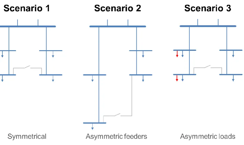
Three scenarios are considered with reference to the simplified HV network, as illustrated in Figure 7:
1. Symmetric feeder impedances and symmetric loads: both feeders are identical, i.e., have the same branch impedances and connected loads. 2. Asymmetric feeder impedances and symmetric loads: the impedances of
the branches of feeder A are increased to: R = 0.5 pu, X = 0.5 pu; this emulates an increase in feeder length. The connected loads are identical. The NOP branch is shown as being longer in Figure 7, but it is not modelled as being longer.
[image:16.595.100.511.266.510.2]3. Symmetric feeder impedances and asymmetric loads: each of the loads connected on feeder A are doubled to 2 MVA. All branch lengths (i.e., impedances) remain equal.
Figure 7: Scenario circuit configurations
3.3.2 Comparison of radial and interconnected operation under different scenarios
This section illustrates the effect of moving from radial to interconnected operation only, and describes the resulting effect on network power flows. The circuits are not at maximum loading, i.e., C2C operation has not been applied to the circuit.
Figure 8: Scenario 1 – radial (left) and interconnected (right)
Due to symmetrical impedances and loads, closing the NOP has no effect; there is no power flow through the branch associated with the NOP, as shown in Figure 8.
3.3.2.2 Scenario 2 – Asymmetric feeder impedances and symmetric loads
Figure 9: Scenario 2 – radial (left) and interconnected (right)
For radial operation, the total demand on feeder A is fractionally higher (approximately 20 kVA) than for scenario 1 due to the additional losses experienced on feeder A as a consequence of its increased impedance.
3.3.2.3 Scenario 3 – Symmetric feeder impedances and asymmetric loads
Figure 10: Scenario 3 – radial (left) and interconnected (right)
In this case, closing the NOP allows the more lightly-loaded feeder prior to interconnection (feeder B) to supply a proportion of the load current of the other feeder via the NOP.
3.3.3 Maximum capacity released under different scenarios for C2C operation
This section assesses the maximum capacity released for each scenario, for both Radial C2C and Interconnected C2C. All loads are scaled up in a distributed fashion until a thermal constraint occurs, as described in Section 3.2.2. A red box around a branch’s power flow label illustrates the presence of a thermal constraint.
3.3.3.1 Scenario 1 – Symmetric feeder impedances and symmetric loads
Figure 11: Scenario 1 – Radial C2C (left) and Interconnected C2C (right)
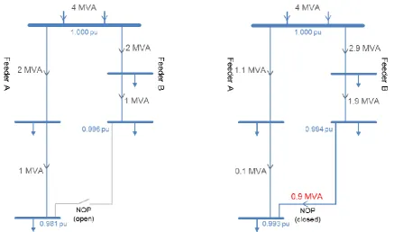
Figure 12: Scenario 2 – Radial C2C (left) and Interconnected C2C (right)
For Radial C2C operation, feeder A experiences slightly higher losses than feeder B due to feeder A’s increased impedance. Consequently, the maximum Radial C2C capacity is dictated by the thermal rating of the first branch of feeder A (5 MVA). Therefore, the total capacity released by Radial C2C operation is 9.9 MVA, slightly lower than theoretical maximum of 10 MVA for symmetric feeders (scenario 1). However, it should be noted that circuit sections with relatively high impedance will tend to have lower thermal ratings, but for simplicity this factor is ignored in this section.
For Interconnected C2C operation, the asymmetry of the feeder impedances increases the power flow through feeder B and thereby “accelerates” the occurrence of a thermal constraint in the first branch of feeder B. Therefore, the maximum demand released by Interconnected C2C operation, 6.9 MVA, is significantly lower than the maximum capacity for Radial C2C operation of 9.9 MVA.
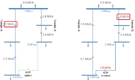
Figure 13: Scenario 3 – Radial C2C (left) and Interconnected C2C (right)
For Radial C2C operation, the maximum capacity is limited by the heavily-loaded feeder. Therefore the maximum Radial C2C capacity is 7.6 MVA. Note that feeder B is relatively underutilised.
For Interconnected C2C operation, feeder B supplies a proportion of the demand connected to feeder A due to the impedances of the interconnected system. The total capacity is limited by the first branch of feeder A. The maximum capacity released by Interconnected C2C operation, 8.9 MVA, is therefore higher than the maximum Radial C2C capacity for this scenario.
3.3.4 Overview of results for the simplified HV network
Table 1 summarises the maximum demand released by Radial C2C and Interconnected C2C for each scenario, using the simplified HV network.
Scenario 1 Scenario 2 Scenario 3 Feeder impedances Symmetric Asymmetric Symmetric
Load arrangement Symmetric Symmetric Asymmetric
Radial C2C 10 MVA 9.9 MVA 7.6 MVA
Interconnected C2C 10 MVA 6.9 MVA 8.9 MVA Table 1: Summary of maximum released demand
The following can be concluded:
If the two feeders comprising the ring circuit are perfectly symmetrical (scenario 1), which is highly unlikely in practice, there is no difference in the capacity released by Radial C2C or Interconnected C2C; closing the NOP has no effect.
For simplicity, the effects of combinations of feeder impedance and load asymmetry are not demonstrated in this section. However, the following general results can be noted:
1. Feeder A higher loading, feeder A higher impedance: interconnected operation can significantly affect feeder power flows; feeder B supplies a significant proportion of the power, via the NOP, to loads connected to feeder A. The circuit sections near to the NOP require the thermal capacity to support this additional power flow. The worst case voltage on feeder A is significantly improved (e.g., from 0.952 pu to 0.986 pu) by closing the NOP. For this scenario, the suitability of Radial C2C or Interconnected C2C operation, in terms of maximising released capacity, depends on the parameters of the specific circuit.
3.4 Results for ENWL C
2C trial circuits
3.4.1 C2C capacity for uniform demand growth
3.4.1.1 Overview of results
Based on analyses of the modelled circuits, Figure 14 illustrates the increase in total demand which is possible using C2C operation, for both radial and interconnected modes of operation, relative to the previously-established base case firm capacity for each ring circuit. The distributions of these results are visualised using box plots, where the coloured box illustrates the range between the first and third quartiles (Q1 and Q3, respectively), and the median value (Q2) is shown as a black line within the coloured box. The ends of the “whiskers” represent the extreme values within 1.5x the interquartile range, i.e., within . Any outliers, defined as lying outside 1.5x the interquartile range, are represented as blue crosses. The mean values are represented by black dots and are labelled.
The N-1 requirement for conventional operation restricts the utilisation of circuit capacity and the deployment of C2C makes significantly better use of the existing assets: a mean increase of 59% for Radial C2C operation and a mean increase of 66% for Interconnected C2C operation4. For clarity, a 100% increase represents a doubling in demand.
Figure 14: Box plots of increase in circuit capacity
The results in Figure 14 highlight that there is significant variation in the available capacity released by C2C operation across all 36 circuits (an increase ranging from 0% to 184%) because the capacity depends significantly on the circuit topology, the load distribution, and the base case firm capacity. For example, a circuit which is relatively heavily loaded near the NOP of the two individual radial feeders would be expected to benefit the most from Interconnected C2C operation.
than by a voltage constraint, compared with the base case. This is due to the occurrence of voltage constraints during the worst case N-1 configurations (see Figure 2) which must be considered for the base case, but are avoided for C2C operation because additional C2C loads are disconnected when the system is operating in an N-1 configuration.
Thermal constraints Voltage constraints
Base case 67% 33%
Radial C2C 81% 19%
Interconnected C2C 89% 11%
Table 2: Proportion of constraint types for 36 ring circuits for uniform demand growth
Section 3.4.1.2 analyses the differences between Radial C2C and Interconnected C2C operation. The cause of the large range for capacity increase values is analysed in Section 3.4.1.3.
3.4.1.2 Comparison of Radial C2C and Interconnected C2C operation
Figure 15 illustrates the increase in demand for all 36 modelled circuits. Although Interconnected C2C operation releases more capacity than Radial C2C operation on average, there are specific circuits where Radial C2C operation releases more demand capacity. It is important to note that these results assume a uniform, distributed addition of interruptible demand.
Figure 15: Increase in total demand with C2C operation
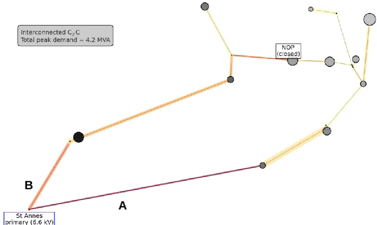
It can be observed that the first circuit section of feeder A, as labelled in Figure 16, experiences a thermal constraint for Radial C2C operation, but feeder B is relatively underutilised. Conversely, for Interconnected C2C as shown in Figure 17, feeder B is able to supply a proportion of the load connected to feeder A via the (closed) NOP. Therefore, for this circuit arrangement, the maximum total demand (indicated by the size of the vertices) is significantly higher for Interconnected C2C operation due to the “balancing” of the power flows in each feeder. This is similar to scenario 3 in Section 3.3.
Figure 16: Graph of St Annes circuit for Radial C2C operation (maximum demand)
B
B
[image:24.595.107.485.474.699.2]symmetrical, and therefore the first circuit sections of both feeders A and B in Figure 18 are at (or close to) the maximum thermal capacity. This indicates that, in this case, Radial C2C operation is effective at maximising the utilisation of the HV circuits.
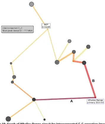
[image:25.595.120.471.236.638.2]Conversely, Interconnected C2C operation causes a change in the power flows due to closing the NOP, which results in the first circuit section on feeder A carrying a relatively higher proportion of the total load current, compared to the base case. As shown in Figure 19, this limits the capacity released for Interconnected C2C because closing the NOP inherently reduces the thermal headroom in feeder A. This is similar to scenario 2 in Section 3.3.
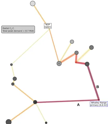
Figure 18: Graph of Whalley Range circuit for Radial C2C operation (maximum demand)
B
Figure 19: Graph of Whalley Range circuit for Interconnected C2C operation (maximum demand)
3.4.1.3 Analysis of range of capacity results
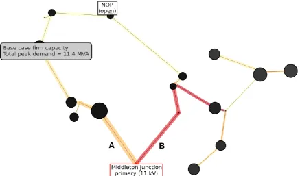
Figure 15 illustrates the extent of the capacity above the base case firm capacity evaluated for Radial C2C and Interconnected C2C operation. It shows a wide range in the results and two example circuits, “Middleton Junction” and “Monton”, are examined here as a way of explanation.
The analysis of the Middleton Junction circuit does not show C2C operation to release any additional capacity for either Radial C2C or Interconnected C2C, relative to the base case firm capacity. This is because connection of the base case firm capacity of the circuit results in each feeder being loaded close to its rating; there is no spare capacity, even in system normal arrangement. The 30% factor in the
B
base case firm capacity would result in a thermal constraint. Therefore, no interruptible C2C demand can be connected to the ring circuit for because a thermal constraint would be experienced on feeder B (and the results show that interconnection does not change power flows significantly).
Figure 20: Middleton Junction circuit for base case firm capacity
Conversely, the Monton ring circuit releases significantly more capacity for both Radial C2C and Interconnected C2C operation, relative to the base case firm capacity, due to a voltage constraint which significantly limits the base case firm capacity (shown in Figure 21) during the worst case N-1 configuration. Additional interruptible demand can be connected during system normal conditions, avoiding the configuration which results in this voltage constraint.
[image:27.595.81.519.141.398.2]
Figure 21: Monton circuit for base case firm capacity
The results for the Middleton Junction and Monton circuits illustrate that the base case firm capacity has a significant impact on the apparent percentage capacity increase released by C2C operation: 0% and 169%, respectively for Interconnected C2C.
3.4.2 C2C capacity for non-uniform demand increase
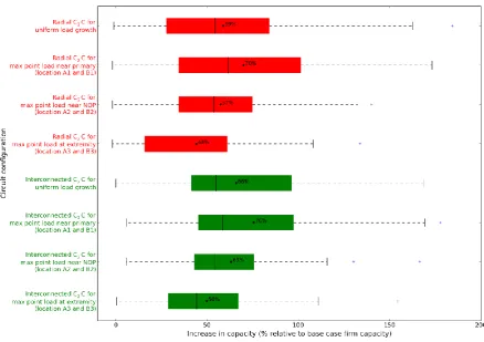
[image:28.595.77.516.185.494.2]Figure 22 illustrates the distributions of point load capacity for each of the three point load locations studied, alongside the results for uniform demand growth presented in Figure 14. The mean value for each distribution is represented by a black dot. The x-axis is the increase in demand, as a percentage relative to the base case firm capacity.
Figure 22: Box plots of maximum C2C demand capacity
Interconnected C2C operation is generally more favourable for supporting point loads, compared to Radial C2C operation. For example, Interconnected C2C operation generally permits larger point load connections at locations near the NOP (locations A2 and B2), i.e., on average 63% compared to 57% for Radial C2C. This is due to both feeders being able to supply load current to the point loads, which generally mitigates thermal constraints, rather than just one feeder as under Radial C2C operation. Furthermore, at the extremities of circuits (locations A3 and B3), Interconnected C2C can typically release more capacity than Radial C2C, 50% compared to 44%, which illustrates that closed ring operation can provide greater flexibility in accommodating additional demand.
Figure 22 illustrates how the “localisation” of demand can affect the released capacity, compared with uniform load growth. For example, at locations A1 and B1, the point load capacity is higher than assuming uniformly demand growth. Point load locations A2 and B2 release slightly less capacity compared to uniform growth and locations A3 and B3 release significantly less capacity (as would be expected from the relatively high impedance between the point of connection and the primary).
3.4.3 Impact of Interconnected C2C operation on demand diversity
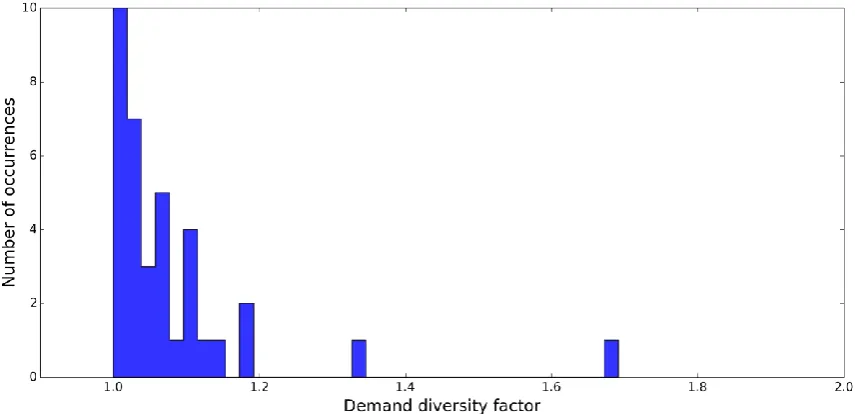
The studies in this chapter assume that the maximum demand connected to each feeder occurs at the same time, without diversity. Interconnected C2C operation has the potential to increase the diversity of demand connected to a ring circuit, i.e., the demand profile over time on feeder A may tend to complement – rather than coincide with – the demand on feeder B, yielding further capacity headroom within the ring circuit. The “demand diversity factor” of the HV ring circuit is defined as:
The aggregate demand is the sum of the half-hourly measurements of both feeders. A demand diversity factor value of 1 is the worst case, indicating that the individual feeder peak demands tend to coincide. A value of 2 is the theoretical best case, indicating that the feeder peak demand values are similar, but the feeder demands are “fully” diverse (which is obviously not likely in practice).
[image:29.595.84.512.529.736.2]Using half-hourly feeder current measurement data from the year 2012, Figure 23 presents a histogram of the demand diversity factor for each of the 36 modelled ring circuits. On average, the demand diversity factor is 1.081, which shows that there is potential for a slight improvement in diversity due to interconnected operation.
3.5 Conclusions
This chapter has described the methodology and results for evaluating the HV network capacity benefits of C2C. A base case has been established which represents the maximum demand that can be connected to a pair of radial HV feeders, without deploying C2C. The capacity increases, relative to the base case, which can be achieved by the deployment of Radial C2C (open ring) operation and Interconnected C2C (closed ring) operation, have been evaluated.
Two complementary methods of modelling additional, interruptible C2C load capacity have been investigated:
1. Uniform demand growth, perhaps reflective of a high penetration of loads such as heat pumps and electric vehicles, which are relatively evenly distributed throughout existing load locations.
2. Non-uniform “point” loads, which may be reflective of relatively large localised loads such as new industrial or commercial customers.
From the results, the following can be concluded:
For either Radial C2C or Interconnected C2C operation, the released capacity depends on the location of existing and additional demand, the circuit topology, and the thermal rating of individual circuit sections.
On average, the practical demand released by Radial C2C should be expected to be up to approximately 44-70% greater than the base case firm capacity.
On average, the practical demand released by Interconnected C2C should be expected to be up to approximately 50-76% greater than the base case firm capacity.
Interconnected C2C operation generally accommodates more demand capacity than Radial C2C operation, when considering all demand scenarios including uniform growth, and point loads connected near the NOP or at circuit extremities. This occurs because Interconnected C2C operation typically supports configurations where one feeder is relatively more heavily loaded than the other feeder comprising the ring circuit; the lower-loaded feeder can supply load current to the other feeder, via the NOP. Such configurations are not possible with Radial C2C, without circuit reinforcement.
The “localisation” of demand connections can affect the released capacity, compared with uniform load growth. Due to the “tapered” design of HV feeder thermal ratings, greater capacity is released for demand concentrated closer to the primary compared to demand concentrated at more remote locations.
Chapter 4: Impact of C
2
C Operation on
Released DG Capacity
4.1 Introduction
This chapter describes the methodology, results, and analysis of a simulation study to evaluate the distributed generation (DG) capacity released by C2C operation applied to 36 actual circuits. A DG “base case” is established which defines the maximum DG which can be connected to circuits without C2C operation, i.e., when there is a requirement for DG to remain connected during N-1 conditions. Therefore, the additional DG which can be connected for C2C operation – where DG may be disconnected during N-1 conditions – can be quantified. This chapter complements the evaluation of C2C demand capacity described in Chapter 3, and contributes to answering the following C2C project hypothesis: “the C2C method will release significant capacity to customers from existing infrastructure”.
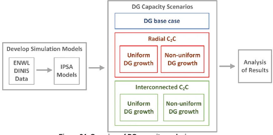
[image:32.595.78.515.454.670.2]The DG capacity improvement for each circuit, relative to the DG base case, has been determined for both “Radial C2C” operation and for “Interconnected C2C” operation, i.e., the effects of operating the network with a closed ring have been evaluated. Two complementary approaches for determining the range of DG capacity which is released by C2C operation have been used for each circuit: distributed, uniform DG growth at existing network locations, and localised, non-uniform “point” DG connected at specific circuit locations. This process is summarised in Figure 61.
4.2 Methodology for establishing DG base case and C
2C
capacities
4.2.1 Overview of methodology
Two complementary approaches have been used to quantify the potential increase in DG capacity released by C2C operation:
1. Uniform growth in DG at all existing secondary substations. This approach is representative of distributed domestic photovoltaic (PV) connections.
2. Non-uniform growth, with DG at just one specific secondary substation on each feeder. This approach is representative of large new DG connections such as wind farms, combined heat and power (CHP), or biomass.
These approaches are intended to mirror the approaches used for evaluating the C2C demand capacity. The DG base case, which is used as a reference for quantifying the increase in DG capacity released by C2C operation, is described in Section 4.2.2. Sections 4.2.3 and 4.2.4 describe the methodologies for evaluating uniform and non-uniform DG growth respectively.
4.2.2 DG base case and assumptions
Figure 25: N-1 configurations for determining the DG base case
No demand is modelled for simulations involving the DG capacity. A maximum HV voltage limit of 1.012 pu is assumed based upon the present HV planning methodology for assessing DG connections5.
4.2.3 C2C operation for uniform DG growth
All connected DG capacity, as established for the DG base case, is uniformly scaled up (using the same multiplicative factor at every DG location) until a thermal or voltage constraint is encountered anywhere in the modelled HV network. This is performed for Radial C2C operation (Figure 26) and Interconnected C2C operation (Figure 27) to establish their respective released DG capacities. For Radial C2C operation, the released DG capacity could be limited by a constraint on either of the two feeders because this represents the level of DG growth where the first reinforcement investment would be required.
Figure 27: Representative DG locations for uniform DG growth of a system operating with Interconnected C2C configuration
4.2.4 C2C operation for non-uniform DG growth
[image:35.595.118.484.501.750.2]Figure 28 illustrates representative locations for specific (or “point”) DG connections. Two representative locations have been selected: the secondary substation at the NOP, and the secondary substation at the furthest extremity from the primary (e.g., at the end of the longest spur). The same locations have been used for “point” loads in the C2C demand capacity evaluation methodology in Chapter 3. Locations near the primary, considered in the non-uniform C2C demand evaluation methodology, are not included in the evaluation of DG capacity, because DG connections near the primary are likely to show very high levels of released DG capacity due to the relatively small impedance between the point of connection and the primary substation and the associated small voltage rise.
Each “pair” of DG connections (A2 and B2, or A3 and B3 as shown in Figure 28) is tested together. This is because Radial C2C operation requires a connection on each radial feeder to appropriately test the DG capacity which is released by the open ring circuit network; consequently, the same DG paired locations are tested for Interconnected C2C operation.
4.3 Demonstration of the effects of interconnection and
C
2C operation on DG capacity using a simplified HV
network
This section provides a simplified overview of the effects of C2C operation on HV network DG capacity using hypothetical, but illustrative, simulated scenarios. The differences and subtleties between Radial C2C and Interconnected C2C operation, in terms of DG capacity released, are highlighted. This section follows the same process as conducted for demand capacity in Section 3.3.
4.3.1 Simplified HV network and assumptions
Figure 29 illustrates a simplified, but representative, HV network with the following properties:
A simplified 11 kV network comprised of two feeders, with two secondary substations per feeder.
A thermal rating of 5 MVA has been used for all branches.
The maximum voltage permitted at any point in the HV network is 1.012 pu.
Initially, a 500 kVA generator, with unity power factor, is connected at each secondary substation. This represents an arbitrary, nominal level of connected generation.
Initially, all branches have the following positive sequence impedances: R = 0.1 pu, X = 0.1 pu (on a 100 MVA base). The branch associated with the NOP (if connected) has the same impedance as all other branches.
[image:37.595.177.420.478.686.2] No load is connected.
Figure 29: Simplified HV network
relevant branch power flows and bus voltages are indicated on Figure 29 and throughout this section.
Three scenarios are considered with reference to the simplified HV network, as illustrated in Figure 30:
1. Symmetric feeder impedances and symmetric DG: both feeders are identical, i.e., have the same branch impedances and connected DG. 2. Asymmetric feeder impedances and symmetric DG: the impedances of the
branches of feeder A are increased to: R = 0.5 pu, X = 0.5 pu; this emulates an increase in feeder length. The connected DG is identical. The NOP branch is shown as being longer in Figure 30, but it is not modelled as being longer.
[image:38.595.89.508.307.564.2]3. Symmetric feeder impedances and asymmetric DG: the capacity of each of the generators connected to feeder A is doubled to 1 MVA. All branch lengths (i.e., impedances) are equal.
Figure 30: Scenario circuit configurations
4.3.2 Comparison of radial and interconnected operation under different scenarios
4.3.2.1 Scenario 1 – Symmetric feeder impedances and symmetric DG
Figure 31: Scenario 1 – radial (left) and interconnected (right)
Due to symmetrical impedances and connected DG, closing the NOP has no effect; there is no power flow through the branch associated with the NOP, as shown in Figure 31.
4.3.2.2 Scenario 2 – Asymmetric feeder impedances and symmetric DG
Figure 32: Scenario 2 – radial (left) and interconnected (right)
For interconnected operation, a proportion of power generated on feeder A is supplied to feeder B (the electrically shorter feeder) via the NOP. Consequently, the power flows in feeder A are reduced compared to radial operation. The worst case secondary substation voltage is improved compared to radial operation, from 1.007 pu to 1.003 pu.
4.3.2.3 Scenario 3 – Symmetric feeder impedances and asymmetric DG
Figure 33: Scenario 3 – radial (left) and interconnected (right)
In this case, closing the NOP allows feeder B, which had less connected DG prior to interconnection, to export a proportion of the power generated on feeder A via the NOP.
4.3.3 Maximum capacity released under different scenarios for C2C operation
4.3.3.1 Scenario 1 – Symmetric feeder impedances and symmetric DG
Figure 34: Scenario 1 – Radial C2C (left) and Interconnected C2C (right)
Figure 10 shows the maximum DG capacities for Radial C2C and Interconnected C2C for the case that feeder impedances and the connected DG are symmetrical.
Closing the NOP has no effect on the maximum DG capacity of the ring circuit, which is 10 MVA in both Radial C2C and Interconnected C2C configurations, with the feeder section between the primary and the first secondary substation being thermally constrained in both cases.
[image:41.595.81.519.438.706.2]4.3.3.2 Scenario 2 – Asymmetric feeder impedances and symmetric DG
Figure 35: Scenario 2 – Radial C2C (left) and Interconnected C2C (right)
higher impedance. The total DG capacity released by Radial C2C operation is 3.2 MVA, which is significantly lower than for the theoretical maximum of 10 MVA for symmetric feeders (scenario 1).
For Interconnected C2C operation, the asymmetry of the feeder impedances increases the power flow through feeder B and thereby “accelerates” the occurrence of a thermal constraint in the first branch of feeder B. However, Interconnected C2C operation mitigates the voltage constraint at the extremity of feeder A. Therefore, the maximum DG demand released by Interconnected C2C operation, 6.8 MVA, is significantly higher than the maximum DG capacity for Radial C2C operation of 3.2 MVA. This is due to the methodology adopted for evaluating Radial C2C operation, as described in Section 4.2.3, which defines the DG capacity as the value just before reinforcement is required on either of the radial feeders.
4.3.3.3 Scenario 3 – Symmetric feeder impedances and asymmetric DG
Figure 36: Scenario 3 – Radial C2C (left) and Interconnected C2C (right)
With the asymmetry in the DG, as shown in Figure 12, for Radial C2C operation, the maximum DG capacity is limited by feeder A, which has a greater level of DG connected. Therefore the maximum Radial C2C capacity is 7.5 MVA. Note that the thermal capacity of feeder B is relatively underutilised.
For Interconnected C2C operation in this scenario, the total DG capacity is still limited by the first branch of feeder A. However, feeder B exports a proportion of the power generated on feeder A due to the impedances of the interconnected system. The maximum DG capacity released by Interconnected C2C operation, 8.8 MVA, is therefore higher than for Radial C2C for this scenario.
Scenario 1 Scenario 2 Scenario 3 Feeder impedances Symmetric Asymmetric Symmetric
DG arrangement Symmetric Symmetric Asymmetric
Radial C2C 10 MVA 3.2 MVA 7.5 MVA
Interconnected C2C 10 MVA 6.8 MVA 8.8 MVA Table 3: Summary of maximum released DG capacity
The following can be concluded:
If the two feeders comprising the ring circuit are perfectly symmetrical (scenario 1), which is highly unlikely in practice, there is no difference in the maximum DG capacity released by Radial C2C or Interconnected C2C; electrically, closing the NOP has no effect on DG capacity.
If one of the feeders comprising the ring circuit has a higher impedance (scenario 2), or if one of the feeders comprising the ring circuit has more DG connected (scenario 3), Interconnected C2C operation will cause a redistribution of power flows and a reduction in the maximum voltage rise – and will thereby generally release more DG capacity than Radial C2C.
4.4 Results for ENWL C
2C Trial Circuits
4.4.1 Uniform DG growth
Figure 37 illustrates the distributions of released DG capacity from the analysis of simulations of 36 C2C trial circuits, as percentage increases relative to the DG base case, using box plots for both Radial C2C and Interconnected C2C operation (see Section 3.4.1.1 for a description of how to interpret box plots). The mean values are labelled.
Figure 37: Summary of DG capacity released by C2C operation for uniform DG growth
The maximum DG capacity values, for a uniform growth in DG which can be connected before a constraint is encountered are presented in as a percentage increase in Figure 38 and in MVA in Figure 39. The types of constraints encountered are documented in Appendix B.
Figure 39: Maximum DG capacity values for uniform DG growth (in MVA)
The results demonstrate that C2C operation provides a significant increase in DG capacity compared to connections based on an N-1 planning approach – an average of approximately 175-225% assuming a uniform growth in DG (where 100% represents a doubling of DG capacity). The requirement for DG to remain connected during N-1 conditions for the DG base case limits the maximum DG capacity, and C2C operation thereby releases significant additional DG capacity.
Similarly to the demand capacity results described in Chapter 3, there is significant variability in the released DG capacity (40-400% for Radial C2C), which is dependent on the specific feeder impedances and DG locations. For example, for the “Griffin” circuit, which includes a relatively long overhead line spur, application of C2C operation releases up to approximately 0.33 MVA (67%) of additional DG capacity; a relatively short cable network such as the “Dickinson Street” circuit is able to release up to approximately 6 MVA (100%) of additional DG capacity.
On average, Interconnected C2C operation releases greater DG capacity (225%) than Radial C2C operation (175%). This is due to the fact that, for Radial C2C operation, a constraint on either radial feeder limits the capacity of both feeders as specified in Section 4.2.3. Furthermore, as illustrated in Section 4.3, Interconnected C2C operation generally benefits from lower voltage rises due to the lower equivalent impedance of the feeders. For example, the “Green Lane” circuit releases significantly more additional DG capacity for Interconnected C2C operation (235%) compared to Radial C2C operation (87%) because closing the NOP mitigates a voltage constraint at the extremity of one of the feeders.
Many of the scenarios shown in Figure 39 may require reinforcement of the primary transformers to accommodate the maximum theoretical C2C DG, especially if other circuits connected to the same primary substation were to accommodate similar levels of DG. For example, the “Middleton Junction” primary has a firm capacity of 23 MVA and Figure 39 illustrates that the circuits under study at Middleton Junction could export up to 11 MVA when maximum DG is connected. If other circuits connected to the same primary substation were to accommodate similar levels of DG, it is clear that the primary transformers may need upgraded to accommodate such growth.
4.4.2 Non-uniform DG growth
[image:46.595.77.514.315.621.2]Figure 40 illustrates the maximum DG released for non-uniform (“point”) DG growth at specific circuit locations, alongside the results for uniform DG growth presented in Figure 37. On average, Interconnected C2C operation releases greater DG capacity than the corresponding Radial C2C scenarios.
Figure 40: DG capacity released by C2C operation
NOP does not exhibit such a high sensitivity to circuit topology and the range of the results is narrower.
4.5 Conclusions
This chapter has described the methodology for evaluating the HV network DG capacity benefits of C2C and the results corresponding to the simulation of 36 C2C trial circuits. A DG base case has been established which represents the maximum DG that can be connected to a pair of radial HV circuits, without deploying C2C, i.e., assuming that DG must remain connected during N-1 conditions. The additional DG capacities, relative to the DG base case, which can be achieved by the deployment of Radial C2C operation and Interconnected C2C operation have been evaluated.
Two complementary methods of modelling additional, interruptible C2C DG capacity have been investigated:
1. Uniform DG growth, perhaps reflective of a high penetration of PV, which is relatively evenly distributed throughout existing secondary substations.
2. Non-uniform “point” DG, which may be reflective of relatively large localised generation such as a wind farm, CHP, or biomass.
From the results, the following can be concluded:
As illustrated for C2C demand capacity in Chapter 3, C2C operation has the potential to accommodate a significant increase in DG connections on HV circuits, and therefore confirms the C2C project hypothesis that: “the C2C method will release significant capacity to customers from existing infrastructure”.
For either Radial C2C or Interconnected C2C operation, the released DG capacity is highly dependent on the circuit topology and the relative modelled DG location.
Interconnected C2C operation will typically release more DG capacity than Radial C2C operation, although there are exceptions to this.
Assuming uniform growth in DG, Radial C2C operation can, on average, release 175% additional DG capacity; Interconnected C2C operation can release 225% additional DG capacity. If such extreme uptake of interruptible DG connections was to occur in HV circuits, and ignoring load connected to the circuit which would “negate” some of the exported power, other system factors such as primary transformer ratings may need to be considered.
Assuming non-uniform DG growth, with point generators connected near the NOP location on each feeder, C2C operation is able to release significant DG capacity; however this would be lower than the DG capacity released by uniform DG growth for both Radial and Interconnected C2C operation.
Chapter 5: Impact of C
2
C Operation on HV
Network Technical Losses
5.1 Introduction
This chapter describes the methodology, results, and analysis for establishing the effects of C2C operation on electrical losses. In particular, this chapter answers the C2C project hypothesis: “the C2C method will reduce like-for-like power losses initially but this benefit will gradually erode as newly released capacity is utilised”.
The analysis distinguishes between the effects of demand-side response (DSR) and interconnected network operation, both of which affect losses. C2C operation is also compared to conventional reinforcement of HV radial networks, which would normally be required to connect the additional demand and DG connections facilitated by C2C. Only technical losses resulting from power dissipation in HV network conductors are analysed; transformer fixed losses and non-technical losses (e.g., from theft or metering inaccuracies) are not taken into consideration. The analysis process is summarised in Figure 41.
Figure 41: Overview of losses analysis process
The methodology for defining the base case firm capacity, Radial C2C, and Interconnected C2C configurations is documented in Chapter 3. It is important to note that the results in this chapter relate to the losses incurred for the maximum demand which can be released by C2C operation and is therefore comparing the “at limit” scenario at a specific point in the future. This is different from the evaluation of losses being undertaken by the University of Manchester which determines cumulative losses over a continuous period of time into the future based upon a demand growth in accordance with a predetermined scenario.
5.2 Effects of HV Network Interconnected Operation on
Losses: Simplified Example
This section provides an overview of the theoretical impact that operating closed HV rings (as opposed to radial systems with open NOPs) may have upon HV network losses. A simplified example ring circuit is given in Figure 42. Its single-phase equivalent circuit is illustrated in Figure 43 (shown for scenario 1 defined below).
Figure 42: Simplified HV ring circuit Figure 43: Single-phase equivalent
The effect of varying the impedance of feeder A or load A is provided in Table 4. The following can be concluded:
1. Closing the NOP for similar feeder and load impedances results in no change in losses. This is illustrated by scenario 1 in Table 4.
2. Closing the NOP for different feeder impedances, but similar load impedances, results in a minor reduction in losses. This is illustrated by scenarios 2 and 3 in Table 4.
3. Closing the NOP for similar feeder impedances, but different load impedances, results in a reduction in losses. This is illustrated by scenarios 4 and 5 in Table 4.
Scenario Feeder A Feeder B Load A Load B
Total Losses NOP Open
Total Losses NOP Closed
1 1 Ω 1 Ω 100 Ω 100 Ω 7.9 kW 7.9 kW
2 0.5 Ω 1 Ω 100 Ω 100 Ω 5.95 kW 5.35 kW
3 2 Ω 1 Ω 100 Ω 100 Ω 11.7 kW 10.5 kW
4 1 Ω 1 Ω 20 Ω 100 Ω 95.4 kW 69.8 kW
[image:51.595.84.513.581.681.2]5 1 Ω 1 Ω 500 Ω 100 Ω 4.12 kW 2.93 kW
Table 4: Effect on per-phase losses for varying feeder A and load A impedances (green
indicates a reduction)
All loads are at the end of the feeders, which is representative of the worst case scenario for losses, assuming radial operation. In practice, loads are distributed along the feeders.
For simplicity, reactive impedances are not considered.
The switch representing the NOP has a resistance of 0.1 Ω when closed, to represent the additional feeder impedance. The losses resulting from this resistance are included in Table 4.
5.3 Methodology for Evaluating C
2C Losses
5.3.1 Overview of methodology
The annual losses for C2C network operation, for the 36 C2C trial circuits, are evaluated using the following process:
1. Simulation of the peak losses for each of the 36 modelled C2C trial circuits. To determine the worst case losses for C2C operation, the maximum demand released by C2C operation for each circuit is considered in this chapter. Uniform demand growth, as described in Chapter 3, has been considered in this evaluation of losses. The maximum demands released by Radial C2C and Interconnected C2C operation, for a given circuit, are different; to allow for a fair comparison, “maximum C2C demand” is defined as the lower of these released demands. Losses are always calculated for system intact conditions. 2. Estimate annual losses for Radial C2C and Interconnected C2C operation,
using the simulated peak losses and historical demand data. This is described in Sections 5.3.2, 5.3.3, and 5.3.4.
3. Estimation of the annual losses in a reinforced radial system supplying the “maximum C2C demand”. I.e., for a fair comparison with C2C losses, the system is considered to be reinforced to support at least the same level of demand as C2C. This is described in Section 5.3.5.
5.3.2 Use of historical demand data
The historical system demand is available in the form of half-hourly averaged RMS current measurements at the primary substations from all 72 trial radial feeders (i.e., each pair of feeders per 36 ring circuits) for the year 2012 (from 1st January 2012 to 31st December 2012). Figure 44 presents an indicative, simplified circuit layout with the demand measurement locations shown. The mean and peak loading data can be extracted for each of the 72 radial feeders and therefore it is possible to estimate the mean and peak loads for the 36 ring circuits. The load factor (LF) and loss load factor (LLF) can be calculated for each radial feeder and for each ring circuit. The annual losses for each circuit can subsequently be estimated from the peak losses determined in circuit simulations [3], [4].
1. Simulate peak losses
2. Estimate annual losses for Radial
C2C and Interconnected C2C
operation
3. Estimate annual losses for equivalent
Figure 44: Ring circuit feeders and current measurement locations
The LF and LLF values for each circuit can be calculated as follows:
The actual annual losses can be estimated using simulation data as follows:
It should be noted that this approach is based on empirical evidence, assuming normal system operation.
It has been assumed that the half-hourly current measurements were all recorded with the 72 feeders operating radially (with the NOP open). To estimate the demand values for the 36 ring circuits (with the NOP closed), the individual current half-hourly data have been aggregated for each pair of feeders that form each ring circuit. This assumes that closing the NOP and forming a ring does not incur any changes in demand.
does not make allowance for possible diversity between the demands on the two radial circuits (see Section 3.4.3 for a discussion of demand diversity).
5.3.3 Processing of historical demand data
Before aggregation of the feeder demand data (as described in Section 5.3.2) and further analysis of losses, it is critical to remove or replace all significantly spurious data points in the feeder current measurements. Even a single erroneous value, such as a measured value “frozen” at a large value such as 700 A, would severely distort calculated values for the circuit peak current. This process has been carried out carefully to avoid, for example, interpolating weekdays using weekends; the interpolation catered for daily, weekly, and seasonal trends. Interpolating from other spurious data points has also been avoided. It is not possible to simply use a moving average when determining the peak demand, because there are several instances of consecutive spurious data. The process also avoids discarding actual anomalies in the demand behaviour.
Figure 45 summarises the process of importing and processing the feeder demand data and further detail is presented in Appendix C.
Figure 45: Importing and processing circuit demand data
5.3.4 Calculated LLF values and annual losses
[image:55.595.88.515.347.484.2]