A parameterized approach to modeling and forecasting mortality

      

City, University of London Institutional Repository

Citation

:

Hatzopoulos, P. and Haberman, S. (2009). A parameterized approach to

modeling and forecasting mortality. Insurance: Mathematics and Economics, 44(1), pp. 103-123. doi: 10.1016/j.insmatheco.2008.10.008

This is the accepted version of the paper.

This version of the publication may differ from the final published

version.

Permanent repository link:

http://openaccess.city.ac.uk/4071/

Link to published version

:

http://dx.doi.org/10.1016/j.insmatheco.2008.10.008

Copyright and reuse:

City Research Online aims to make research

outputs of City, University of London available to a wider audience.

Copyright and Moral Rights remain with the author(s) and/or copyright

holders. URLs from City Research Online may be freely distributed and

linked to.

City Research Online: http://openaccess.city.ac.uk/ [email protected]

A parameterized approach to modeling and forecasting mortality

P. Hatzopoulos

a

, S. Haberman

b

a

Department of Statistics and Actuarial-Financial Mathematics, University of the Aegean, Samos, 83200, Greece

b_{Faculty of Actuarial Science and Insurance, Sir John Cass Business School, City University, 106 Bunhill Row, London}

EC1Y8TZ, UK

Abstract

A new method is proposed of constructing mortality forecasts. This parameterized approach utilizes Generalized Linear Models (GLMs), based on heteroscedastic Poisson (non-additive) error structures, and using an orthonormal polynomial design matrix. Principal Component (PC) analysis is then applied to the cross-sectional fitted parameters. The produced model can be viewed either as a one-factor parameterized model where the time series are the fitted parameters, or as a principal component model, namely a log-bilinear hierarchical statistical association model of Goodman (1991) or equivalently as a generalized Lee-Carter model withp interaction terms. Mortality forecasts are obtained by applying dynamic linear regression models to the PCs. Two applications are presented: Sweden (1751-2006) and Greece (1957-2006).

Keywords: Mortality forecasting; Generalized Linear Models; Principal Component analysis; Dynamic linear regression; Bootstrap confidence intervals.

1. Introduction

The changes in mortality rates over time need to be accurately measured and projected, in order to inform the choice of mortality bases for a variety of disciplines and applications (e.g. in the life insurance and pensions industries, government policy and planning). Downward mortality trends have been gradually decline since the start of the twentieth century, but there is evidence that such trends may not be uniform across the age groups. As mentioned by Wilmoth (2000), these gains in longevity are the result of a complex array of changes (standards of living, public health, personal hygiene and medical care), with different factors playing major or minor roles in different time periods.

Mortality rates exhibit strong age patterns and various researchers have developed methods to capture this structure and use it in forecasting. Two important, general approaches have been developed for modeling and forecasting: the curve fitting approach and the principal component (PC) approach. The model fitting approach involves fitting parametric curves to the age-specific mortality rates and the PC approach involves computing PCs to obtain a linear transformation of the data in lower dimension and simplified structure.

The fitting of curves to mortality rates has a long history in demography and actuarial science, going back to the efforts of DeMoivre (1725) and Gompertz (1825). The objectives have usually been to estimate mortality curves with limited data, or to graduate (smooth) irregular curves of directly estimated rates. Thus, Cramer and Wold (1935) fit Makeham curves to cross-sectional Swedish mortality data for ages 30 and above, and then extrapolate the fitted parameters using logistic functions of time. Similarly, McNown and Rogers (1989) fit an eight-parameter Heligman-Pollard (1980) curve in age effects to cross-sectional US mortality for 86 years. After differencing to achieve stationarity, the eight univariate time series are estimated by ARIMA models and extrapolation is then used for forecasts. McNown and Rogers (1992) forecast total mortality and five cause-specific mortality rates, using a non-linear model, similar to the Heligman-Pollard (1980) curve with nine parameters, by fixing six parameters and modelling only the time dependence of level parameters by univariate ARIMA models.

the parameters is theoretically possible but seriously complicates the approach and can lead to computational intractability. Alternatively, Renshaw et. al (1996) propose a two-explanatory variable model with two multiplicative terms: a graduation term and an age-specific trend adjustment term.

As discussed by Bell (1997), application of PCs analysis to mortality rates goes back at least to Ledermann and Breas (1959), who perform their analysis not on time series data, but with life table data from many countries, both developed and developing. Sinamurthy (1987) pursues a similar analysis with fertility data from different countries. Bozik and Bell (1987) develop a PC approach for time series forecasting of age-specific fertility rates. This approach has been extended by Bell and Monsell (1991), where it is used in forecasting age-specific mortality rates. Lee & Carter (1992) explore a modified version of this approach for forecasting mortality rates, which Lee (1992, 1993) has also applied to fertility rates. Lee and Carter propose a simple model for describing the secular change in mortality as a function of a single time index:

, ( ,

log( )- )

tx t x x x t t x

z  m    kappa 

where



_x(

kappa

)

_t

 

s u x v t

( )



( )

and s u x v x, ( ), ( ) denote the singular value and respective left and right singular vectors of

z

_tx. The time component (

kappa

)

_t is an index of the level of mortality, the ‘dominant temporal signal’ and captures the overall time trend in log mortality at all ages,



_x is a set of age-specific constants describing the general pattern of mortality by age,



_x is a set of age-specific constants describing the relative speed of change at each age (and related to the proportion of the change in overall log mortality attributable to agex), and _{t x,} is the residual at agexin yeartand denotes the deviation of the model from the observed log-central death rates and is assumed to be a white noise process with 0 mean and relatively small variance (Lee, 2000).

The main statistical tool is least-squares estimation via singular value decomposition (SVD) of the matrix of the

log age specific observed forces of mortality, applying the constraints (

)

_t

0

t

kappa





, _x

1

x







in order to

ensure identifiability of the model, and estimating the parameter



_x by the average log-central death rates at each age over time, together with Box-Jenkins ARIMA modeling of the time series component (

kappa

)

_t. We note that in the literature, prominence is given to the random walk with drift time series models, as initially advocated by Lee and Carter (1992). Once



_x and (

kappa

)

_t are estimated, under the above constraints, (

kappa

)

_t is further adjusted to ensure that the actual total deaths are identical to the total expected deaths for each calendar year within the data set, as a basis for comparing actual and expected deaths.

The Lee and Carter (1992) and Bozik and Bell (1987) approaches can be viewed as being similar. They differ in the way that Lee-Carter approach first subtracts out age-specific means (



_x) and uses one PC. As discussed by Bell (1997), given that a one-PC approximation is to be used, subtracting out the age-specific means is definitely recommended. Since the use of two PCs provides, by definition, the best two-dimensional linear approximations, the Lee and Carter approximation has an accuracy that lies between the accuracy provided by approaches using one and two PCs obtained without removing means. Subtracting the means is useful with low-dimensional PC approximations, but it becomes less important when more PCs are used, and is unnecessary if all of the PCs are used as in Bell and Monsell (1991).

estimated by maximum likelihood estimation for Poisson-distributed errors. Brouhns et. al. (2002) and Renshaw and Haberman (2003a) have each implemented similar alternative approaches to mortality forecasting, based on heteroscedastic Poisson (non-additive) error structures.

Violations also exist in the LC model from the assumption that the age component



_x is invariant over time, and that the mortality improvement at all ages will follow a fixed pattern (Lee and Miller 2001). In the LC method, the SVD estimates reduce to, in essence, simple means and standard deviations and these estimates are insensitive to the more subtle aspects of mortality trends and it has been argued that they form a crude basis for mortality projections (Jong & Tickle, 2006). In fact, the mortality experience of the industrialized world over the course of the twentieth century would suggest substantial age-time interactions: the two dominant trends affecting different age groups at different times (Booth et. al. 2002). Several modifications have been proposed to cope with these limitations of the LC model. Renshaw and Haberman (2003a) incorporate the age differential effects, introducing a double bilinear predictor structure, (age-specific enhancement) into the LC forecasting methodology by optimizing the Poisson likelihood, as opposed to optimizing the Gaussian likelihood, as under the LC approach, and compare the results. The LC approach fails to capture and project the most recent upturn in crude mortality rates, roughly in the age range 20-39 years, as established in the raw data over the last quarter of the century and widely attributed to increases in the number of suicides and deaths related to HIV infection and AIDS. This is particularly noticeable in the case of UK male assured lives (with policies of duration 2+ years) where the 1stsingular value accounts for 74% of the total variance. However, while the fitting of such augmented systematic model structures is straightforward, the generation of the subsequent univariate time series forecasts, based on such structures, is potentially problematic (Renshaw and Haberman 2003a). In many developed countries (including UK, US, Japan and Germany), there is evidence of a cohort effect – thus, in the UK, generations born between 1925 and 1945 approximately seem to have experienced more rapid mortality decreases than earlier or later generations. Renshaw and Haberman (2006) incorporate this effect by developing an age-period-cohort version of the LC model which provides an improved fit to the data than the basic LC model. Similarly, Yue et al (2008) apply the Bell (1997) approach to several countries, and propose a jump model to the mortality rates, including two second-order interaction terms (age-period and age-cohort). They suggest that the reduction shift of ages for different time periods can be treated as a “cohort” effect, introducing an age-period-cohort (APC) model. Also, Hyndman and Ullah (2005) use several PCs to capture the differential movements in age-specific mortality rates. They smooth first the observed log-mortality rates with constrained and weighted penalized regression splines and they decompose the fitted curves using functional principal component analysis.

Further, the LC model assumes that the logarithms of the mortality rates are approximately a linear function of time (and the mortality rates of all ages eventually go to 0). Several authors indicate a marked departure from linearity in the dominant time component, casting doubt on the ‘universal pattern’ of decline and hence the general applicability of the linear forecasting model. Thus, some authors prefer to have a restricted fitting period. Thus, Booth et. al. (2002) propose a method for determining the optimal fitting period in order to address non-linearity in the time component.

Recently, many authors have proposed new approaches to mortality forecasts, utilizing (nonparametric) smoothing. Currie et. al (2004) use bivariate penalized B-splines to smooth the mortality surface in both the time and age dimensions within a penalized GLM framework. Hyndman and Ullah (2005) smooth the observed log-mortality rates with constrained and weighted penalized regression splines. De Jong and Tickle (2006) introduce a state space framework using B-spline smoothing.

which contain as much information as possible and explain the inherent variation of the mortality rates. The modelling of the estimated parameters trends in time is accomplished by applying PC analysis to the table of the parameters estimates, where each row denotes the number of years, and each column denotes the number of fitted parameters needed for each year. In this way, we reduce the dimensionality of the problem by focusing on the linear combinations of the estimated parameters leading to the PC terms. These are then used for modelling and forecasting purposes. We utilize dynamic linear regression (dlr) models, for modelling and forecasting the PCs. The statistical treatment of the dlr models is based on the state space framework and the Kalman filter.

The remainder of the paper is organised as follows. In section 2, we analyse the methodology proposed for the parameterized approach of modelling central mortality rates and we define the particular class of dlr models which we utilize for forecast purposes. In section 3, we illustrate two applications based on Sweden and Greece mortality experiences and incorporate an ex-post study to define the optimum fitting period for the long-historical mortality data from Sweden. In section 4, we offer a discussion and some concluding remarks.

2. Methodology

The data for analysis, which are denoted by

(

d

_xt

,

R

_xt

)

, comprising the observed number of deaths,

d

_xt, with matching central exposures to the risk of death,

R

xt, defined over rectangular data grids (t,x), witht ranging over the individual calendar years range [

t

1,

t

n] and x ranging over the (grouped) age range [

x

1,

x

n]. If we assume that for any (grouped) age x and calendar year t, the force of mortality is constant, i.e.

( )

( )

x c

t

x

t

m





m

for 0 c g, where g is the width of the age grouping (for integer ages g=1), then the

force of mortality is identical with the central rate of mortality:

m

_x

( )

t



_g

m t

_x

( )

. We model, the response variates, the actual number of deaths as independent realizations of Poisson random variables,

D

xt, conditional on

R

_xt, i.e.

D

_xt



Poisson R

(

_xt



m

_x

( ))

t

(Brillinger, 1986), for each calendar year independently. In this way, the calendar time enters the model as a factor.

In many actuarial mortality investigations, the data available do not consist of the actual deaths and the exposures based on individual lives. In studies of insured lives or annuitants for example, each policyholder may have more than one policy and any claim may subsequently give rise to more than one "death". The actual data available, for this kind of investigation, are the number of policies, ceasing through death and the corresponding exposed to risk based on policies. Similarly, overdispersion can occur in modelling data when sampling a Poisson process (Cox, 1967) over an interval whose length is not fixed, but is itself random (the alternative Gamma distribution for the central exposures is discussed in Renshaw et. al., 1997). Therefore, in these situations, a simple Poisson process does not describe the real process under which the data are generated. In the context of a Poisson GLM, this feature is described as over-dispersedPoisson process. Renshaw (1992), describes a methodology of joint modelling of the mean and of the dispersion, using the over-dispersed Poisson model for policies, such that

(

xt

)

x

( )

xt

E D



m t



R

and

Var D

(

xt

)

 

j

t

E D

(

xt

)

where the over-dispersed parameter

j

_t is independent of the response variate, and is the theoretical equivalent of the empirical variance ratiordiscussed by Forfar et al (1988) and can be estimated by the ratio of the quasi-deviance divided by the associated degrees of freedom. If j_t is treated as a constant, it does not have any effect on the values of the parameter estimates in the linear predictor, only on the standard errors and confidence intervals, which might differ seriously if this effect is not taken into account (Cox,1983). Renshaw (1991) describes the implementation of

m

x

( )

t

graduations, using generalized linear model techniques, based on

these distributional assumptions. Using log link predictor formulae, which is the canonical link for the Poisson distribution; the estimates are unique. The predictor structure is:

( )

log( (

))

log(

( ))

log(

)

log(

( ))

x

t

E D

xt

R

xt

m t

x

R

xt

m t

x

h











in which the

log(

R

xt

)

term is treated as an offset. This implies that the rates of mortality are modelled as an

each calendar year independently, using an orthonormal polynomial structure in age effects. That is, we

investigate predictor structures of the type _{1 1} 1

( )

( )

k

j j

j

b

_

t

L

_

x







, where L_j1( )x denotes an orthonormal, (zero-centered forj=2,…,k), polynomial of degreej-1,forj=1,2,…,k, leading tograduatedmortality rates:

1 1

1

ˆ ( )

exp

( )

( )

k

x j j

j

m t



_

t

L

_

x















_

_











(2.1)

for each calendar year independently. The random variables



_j1

( )

t



b

ˆ

_j1

( )

t

are the fitted variables at timet, for j=1,2,…,k. With



( )

t



b t

ˆ

( )

we denote the multivariate random variable at time t, where

0 1 1

( , , , )

( )

( )

( )

_k

( )

b t



b t b t



b

_

t

 Rkthe unknown vector of the parameters. The integrals, which are needed for the calculation of the norm of the polynomials, are computed using discretization. Under this modelling, the design matrix

L



(

L x L x

₀

( ),

₁

( ),...,

L

_k1

( ))

x

(of order x byk) consists of k-dimensional orthonormal vectors. We note that, in comparison with LC-methodology, this modelling ensures that the actual total deaths are identical to the total expected deaths for each calendar year.

The choice of employing orthonormal polynomials to form the linear predictor’s vector basis is justified by the fact that the standard errors of the multivariate random variable



( )

t

, for each calendar yeart, are on the same scale, i.e. the standard errors of the parameters have about the same values, and this assists the use of PC analysis on the variance-covariance matrix of the



( )

t

. We note that, the variance-covariance matrix has the

form

Var

( ( ))



t



(

L V L



_t1

)

1, where

V

_t



diag u

(

_xt

)

,

u

_xt



Var D

(

_xt

)



dr

_xt



ˆ

_t

E D

(

_xt

)

dr

_xt







 



ˆ

_t

R

_xt



m t dr

ˆ ( )

_x



_xt, and dr_xt the associated deviance increments defined us

ˆ log( ) ( ˆ ( ))

ˆ ( )

xt

xt t xt xt xt x

xt x d

dr d d R m t

R m t

  

 _     _



 .

A restriction for the standard errors of the estimated parameter vector



( )

t

in time should be that they must represent only random fluctuations and not be associated with any model risk or any sampling errors. Thus, assuming that the model fit is adequate, and from the fact that the standard errors depend on the size of the expected deaths, then the total central exposures, in each calendar year under investigation must have close values, or equivalently the population must show a relative stationarity.

from the crude mortality rates and to justify the cross-sectional graduation process, and also if we need a parsimonious parameterized model structure.

As has been pointed out (see Pitacco, 2004), the uncertainty in modelling and forecasting mortality rates is attributable to random fluctuations, “process risk”, uncertainty in estimating the values of the parameters, “parameter risk” or to uncertainty in the choice or structure of the model, “model risk”. Under the proposed parameterized approach, in order to minimize the “model risk”, we can investigate the appropriateness of the ‘law of mortality’ by various statistical tests (chi-square test, run test, sign test) and utilize scaled deviance residuals.

Fitting an orthonormal polynomial structure in age effects, for each calendar year, we produce a matrix, of order

nbyk, of b_j1( )t entries: B{b_j1( )}t , fort=1,2,…n and j=1,2,…,k. and a matrix, of ordernbyx, with entries

m t

ˆ ( )

_x :

M



exp



B L







or

log(

M

)

 

B L



, fort=1,2,…n and x=

x

₁,…,

x

₂.

Noting the properties of GLMs, each cross-sectional vector of the estimated parameters is a k-dimensional random variable which follows asymptotically a multivariate k-dimensional normal distribution:( )t N_k( ( ),b t Σ_t), where

Σ

_t is the associated covariance matrix, at each different calendar year

t. Let _j1:(_j1(1),_j1(2),,_j1( )n ) denote the random process, for eachj=1,2,...,k.

In this context, the modelling of the estimated parameters trends in time is accomplished by applying PC analysis (in association with the covariance matrix) to the table of the fitted parameters B{b_j1( )}t , where each row denotes the number of years, and each column denotes the number of fitted parameters needed for each year. We usually use the rescaled vectors, say



r_j1





_j1





_j1, for each j=1,2,...,k, where

1 ( 1(1), 1(2), , 1( ))

j j j j n

           and



j1 the arithmetic mean value of the j1 vector (treating them as constants), producing the rescaled matrix Br   B b {br_j1( )}t {b_j1( )t b_j1}, where



0

,

1

,...,

k



b



b b

b



is the vector of the mean values,

for each j=1,2,...,k and for each calendar year

t=1,2,…,n, with associated covariance matrixΣ.

PC analysis involves the computation of the singular value decomposition of a data set, usually after mean centering the data for each attribute. PC analysis can be used to reduce the dimensionality of a data set by retaining those characteristics of the data set that contribute most to its variance, by keeping lower-order principal components and ignoring higher-order ones (Mardia et. al. 1997). Such low-order components often contain the “most important” aspects of the data and we keep a “small” subset of them, say p(<k), which explains the “majority” of the variances (see section 3.4). Thus, we apply eigenvalue decomposition, to the covariance matrixΣ, with the associated matrix of eigenvectors

P



[

e e

₁, ₂,,

e

_k] and vector of eigenvalues



 1, 2,...,k





  . The decomposition produces a matrix of PC scores, of order nbyk:

Y



B

r



P

, leading to the equations

Y t

( )

 

P





r

( )

t

, where Y t( )



Y t Y t₁( ), ₂( ),...,Y t_k( )



 the vector of the PC scores in yeart, and

Y t

_i

( )





r

( )

t

'



e

_i for each calendar yeart=1,2,…,n and each PC i=1,2,…,k. We note that the vectors of PC scores, Y t( ), are normally distributed since they are linear combinations of the k-dimensional normally distributed vector random variables



r

( )

t

. Thus, the result of the principal components analysis to the fitted GLM parameters is the creation of a new multivariate random process, the principal component random vectors,

( )

Y t , which are normally distributed, and then we examine the PCs for possible trends in time. The PC analysis ensures that

Cov Y Y

( , )

_{i l} =0, for

i



j

, and, from the normality property, we obtain that the stochastic processes

( )

i

The vector of the graduated log-central death rate at each age in yeartis then of the form





ˆ

log(

m

_t

) =

L





( )

t

 

L

 



r

( )

t

   

L



L



r

( )

t

    

L



L P

Y t

( )

  

A

G

Y t

( )

(2.2)

where

A

 

L



or

A x

( )



L x



( )





,

G  L P



g g₁, ₂,...,g_k



with columns

g_i  L e_i

and values

( )

( )

i i

g x



L x e





, and where

L x( )



L x L x₀( ), ₂( ),...,L x_k( )





denotes the vector of the design matrix’s

x

-row. We note that the matrix of eigenvectors

P

is a projection matrix which transforms the matrices

r

B

and

L

into PC scores and age-specific scores respectively. Thus, we derive the structure

1

ˆ

log( ( ))= ( ) ( ) ( )

k

x i i

i

m t A x g x Y t









Keeping a “small” subsetp(<k) of the PCs, which explains the “majority” of the variance (see section 3.4), leads to:

1

ˆ

log( ( ))= ( ) ( ) ( ) ( )

p

x i i x

i

m t A x g x Y t  t







  (model 1)

The disturbance term



_x

( )

t



N

(0,

v

_x

)

, is the error component at age x in yeartand denotes the deviation of the model represented by the excluded PCs, which are normally distributed with zero mean and variance

v

_x

,

estimated by

2

1

ˆ

( )

k

x i i

i p

v

g x



 







.

The model that we have derived can be viewed as a variant of the

Lee-Carter model withpinteraction terms. According to the LC method, the first PC,

Y t

₁

( )

, denotes the index of the level of mortality that captures the overall time trend in log mortality at all ages. In that case, the time components

Y t

_i

( )

are stochastic Gaussian processes, which are linear combinations of the (rescaled) cross-sectional fitted parameters and the eigenvectors. A x( ) is a set of age-specific constants which are linear combinations of the mean fitted parameters and rows of the design matrix, describing the general pattern of mortality by age.

g x

_i

( )

is a set of age-specific constants which are linear combinations of the eigenvectors and the rows of the design matrix. The first function

g x

₁

( )

denotes the proportion of the change in overall log mortality attributable to agex. The remaining interaction terms

g x Y t

_i

( )



_i

( )

, for i=2,…,p, incorporate the age differential effects, including age-period interaction terms. The importance of each component can be measured by the PC variances



_i

,

for i=2,…,p, which define the goodness of approximation as judged by the ratios

1 2 1

...

...

p p k

l









 



 

, wherep the number of components used and 1 ... p. The PCs can be considered also as ‘factors’ (common characteristics as analysed in factor analysis) that describe certain features of the mortality process. These ‘factors’ can be labelled in agreement with the age components

g x

_i

( )

.

From the non-reduced model (1), after some simple algebraic manipulations we obtain:

, 1

1 1

ˆ

log( ( )) = + ( ) ( ) ( )

k k

x j i i j

j i

m t   x e Y t L _ x

 

 

 _   _

 

 

1, 0 , 1

1 2

+ ( ) ( ) ( ) ( )

k k

i j i j i

i j

x e L x e L x Y t

  

 

 

  _    _

 





, i.e.

1

ˆ

log( ( ))= + ( ) ( ) ( ) ( )

k

x i i

i

m t   x b t f x Y t





1

ˆ

log( ( ))= + ( ) ( ) ( ) ( )

k

x i i i

i

m t   x b t   x  t





 



 (2.3)

where   ₀ L₀, _{1 1}

2

( )

( )

k

j j

j

x

L

x





 









, _{0 1,}

1

( )

( )

k

i i i

b t

L

e

Y t











, , 1 1

( )

( )

k r

i j i j

j

Y t

e



_

t









_{, , 1}

2

( )

( )

k

i j i j

j

f x

e

L

_

x









, 1 2

( )

( )

( )

n i i x i x x

f x

x

f

x









, 1 2

( )

( )

( )

(

1)

( )

n i i i t i i t t

Y t

Y t

t

n

Y

t











 



and 1 2

( 1) ( )

n

x

i i i

x x

n f x

 



   



The model now can be viewed as a member of the class of log-linear models, namely a hierarchical statistical association model for a two-way cross-classification table with age and time being the two main random effects, similar to the so-called (unweighted)association modelof Goodman (1991).

The component  is the overall mean, the components ( )x and b t( )are the age main effect and time main effect, which comprise the independent or additive model, and the



_i

( )

x

and



_i

( )

t

are viewed as scores relating to thexthage andtthcalendar year categories respectively, which embody the interactions between age and time. ( )x gives the age profile and represents deviations from the overall mortality mean 

,

that are attributable to agex, and b t( ) is an index of the level of mortality in time effects that captures the overall time trend in log mortality at all ages (with values that represent deviations from the overall mortality mean that are attributable to calendar yeart). The components



_i

( )

x

describe relative deviations from the general age pattern of mortality (the independent component) and they indicate the sensitivity of the logarithm of the force of mortality at age x to variations and trends in the time index



_i

( )

t

. They modify the main age profile and represent the age-specific patterns of mortality changes. The shape of the



_i

( )

x

profile tells which rates respond rapidly and which slowly over which period of time, in response to particular trends in



_i

( )

t

. For negative



_i

( )

x

values, increasing (decreasing) values of



_i

( )

t

represent a faster rate of improvement (deterioration) relative to independent model, and for positive



_i

( )

x

values, increasing (decreasing) values of

( )

i

t



represent a faster rate of deterioration (improvement) relative to independent model with relative degree of deterioration (improvement) as indicated by the first derivative of the



_i

( )

t

’s.

For identifiability reasons, the age and time scores are zero-centered normed scores subject to the constraint that the age and time scores are internally orthogonal:

1

( )

n x i x x

v x





=0, 1 2

( )

1

n x i x x

v

x







, 1

( )

0

n t i t t

t









, 1 2

( )

1

n t i t t

t









, 1

( )

( )

0

n

x

i j

x x

v x v x









and

1

( )

( )

0

n t i j t t

t

t













 i j (2.4)

the time variations. The



_i parameters are singular values of the matrix of the residuals (from the independent model) D, defined by

D



(

d

_xt

)





log(

m t

ˆ

_x

( ))-

 



( )

x



b t

( )



, with associated singular vectors



_i

( )

x

and _i

( )

t

. The eigenvalues parameters



_i2, can be used as an index of the importance of each interaction term

and define the goodness of approximation as judged by the ratios

2 2

1 2

2 2

1

...

...

p p

k

r  

 

  

  , wherepis the number of

interaction terms used :



_i2

 

...



_p2. The ratio offers a guide as to how many interaction terms are to be included in the model, applying a similar methodology from PC analysis. A possible criterion for the optimum choice of the number of eigenvalues could be to look at the pattern of eigenvalues (a scree plot) and see if there is a natural breakpoint, or to identify clusters of eigenvalues and keep those clusters that explain the majority of the deviations from the additive model. A final choice would be motivated by the possible interpretations of the associated



_i

( )

x

and _i

( )

t

values. After retaining the most important interaction terms, we derive the model structure:

1

ˆ

log( ( ))= + ( ) ( ) ( ) ( ) ( )

p

x i i i x

i

m t   x b t   x  t  t





 



  (model 2)

Thus, forecasts for the _i

( )

t

time series (or equivalently, for the

Y t

ˆ ( )

_i time series) will produce forecast values for the mortality rates. Any forecast stochastic model for the PCs can lead to predicted mean values, say

ˆ( )

Y t , for each calendar year, with associated estimated variance-covariance matrices Var Y t( ( ))ˆ . From the predicted mean values of the PCs, we can obtain the ‘predicted values’ of the original parameter estimates from the mathematical relationship:

B

ˆ

r

 

Y P

ˆ

, under the assumptions that the eigenvector matrix P will not change its structure during the forecasting period. From the Cayley-Hamilton Theorem we have, for the relationship Σ = PΛP, that, if a real functionf(x)is given by a power series:

f x

( )

=

a

₀

   

a x a

_{1 2}

x

2



...

then f( )Σ = Pf( )Λ P. This property implies that, any changes in the covariance matrix Σ, during the forecast period, of the form

f x

( )

=

a

₀

   

a x a

_{1 2}

x

2



...

, will not affect the matrix of eigenvectors P. It seems, under this property, that the predicted values

B

ˆ

r (and also the predicted Yˆ values) have a degree of robustness in terms of structural changes of the covariance matrix Σ during the forecast period. The linear transformation

B

ˆ

r

 

Y

ˆ

r

P

, where the matrix rP, of orderkbyp, denotes the reduced form of the matrix of eigenvectors by keeping only the firstpeigenvectors, leads to the set of equations



ˆ

r

( )

t



r

P



Y t

ˆ

( )

for each calendar yeart, which form a new,k-dimensional, normally distributed, random process. Thus, alternatively, the predicted log-mortality can be viewed as a one-factor parameterized model, where the time series are the fitted parameters:

1 1

1

ˆ

ˆ

ˆ

log(

( ))=

( )

( )

k

x j j

j

m t



_

t

L

_

x







(model 3)

where _{1 , 1}

1

ˆ _{( )} p ˆ_{( )}

j j i i j

i

t e Y t

   







  . The estimated variance-covariance matrices of the cross-sectional

estimated parameter vectors, for each calendar yearstare



1



ˆ

r

_{( )}

r

ˆ

_{( )}

r r

ˆ

_{( ) ,...,}

ˆ

_{( )}

r

p

Var

_





t

_





P



Var Y t

_





_



P





P



diag Var Y t



_



_

Var Y t

_



_





P



(2.5)

and the estimated variance of the predicted log-mortality rates structure, for any grid of values ( , )x t are

ˆ

ˆ

ˆ

log(

_x

( ))

( )

( )

Var



_

m t

 

_

Var L x



_







t



_

If the random vectors

Y t

ˆ( )

belong to the class oflinear estimatorsin the observations

Y t

_i

( )

, then the random vectors



ˆ( )

t

and

log(

m t

ˆˆ

_x

( ))

are also asymptotically normally distributed, and confidence intervals can be derived.

Also, from the predicted mean values and the estimated variances of the PCs, we can obtain the ‘predicted values’ and the estimated variances of the time main effects, under the independence assumption for the predicted mean values of the PCs:

0 1, 1

ˆ

_{( )}

p

ˆ

_{( )}

i i i

b t

L

e

Y t











and 2_{0 1,}2

1

ˆ

_{( )}

p

ˆ

_{( )}

i i

i

Var b t

L

e

Var Y t















_



_







(2.7)

For forecast purposes, for each PC, we advocate a specific class of dynamic linear regression (dlr) models:

ˆ( )

( )

( )

( )

Y t



a t



b t t

 

e t

(2.8) for each calendar yeart(the so-called regressor), with stochastic time variable parameters (level and slope) that follow an autoregressive-moving average process. Newbold and Bos (1985) argue that it is difficult to distinguish among different members of the autoregressive-moving average class of models to represent stochastic parameter behaviour, and their view is that, for the great majority of problems met in practice, a regression model with stochastic parameters following a first-order autoregressive process should provide an adequate representation of the available data, though on occasion one or more additional autoregressive terms may be required. Experiments with various mortality experiences have shown that the PCs can be represented adequately under the dlr model structures, with the stochastic parameters following a first order autoregressive process, for stationary PCs, or a random walk process, for non-stationary PCs:

1

( )

(

1)

( )

a t

 



a t

 



t

and

b t

( )





₂



b t

(

 

1)



( )

t

(2.9)

All of the components are stochastic and the disturbances driving them (



_e2,



_2 and



_2) are assumed to be mutually uncorrelated. The crucial feature of the model is the signal-noise ratio (or noise-variance ratio

hyper-parameters)

2

1 ₂ e q  

 and

2

2 ₂

e q  

 .

If the correlation coefficients  are less than 1 in absolute value, then the model is called a first-order autoregressive model, where the strength of the correlation between two values of the time series is decreasing as their distance apart in time increases. If  is equal to 1 the model is called a ‘random walk’ model (the “border line non-stationary” case) and if both the coefficients are equal to one then the model reduces to the

local linear model with reduced form - an ARIMA(0,2,2) process (Harvey, 1991). Random walk models are best thought of as describing a situation in which changes from one period to the next are white noise and are therefore unpredictable in terms of past changes. In this case, we assume that the (Gaussian) PCs incorporate local linear trends, and we remove those linear trends in time using dlr models and Kalman filter techniques. In the special case when



_2=0, the model reduces to an ARIMA(0,1,1) model plus constant term (Harvey, 1991). This particular case has been found to be very popular in modelling the PCs trends. However, it is possible that  exceeds one in absolute value, in which case the model is called “explosive”, but these models are not useful for representing real data in the social sciences (Newbold and Bos, 1985).

The effect of ( )t is to allow the level of the trend to shift up and down, while ( )t allows the slope to change. The larger the variances, the greater the stochastic movements in the trend. If the white noise of the stochastic parameter is equal to zero, then we consider the corresponding parameter constant and, if both the white noises of the stochastic parameters are equal to zero, then the model reduces to an ordinary linear regression model.

Dynamic linear regression models are simple models from the wider class of models known as principal structural time series models. Structural time series models are set up in terms of components, such as trends and cycles, which have a direct interpretation. The principal univariate structural time series models are simply regression models in which the explanatory variables are functions of time and the parameters are time-varying. State space models employ the Kalman filter technique to provide a computationally efficient framework through which we can derive estimates of the stochastic parameters and predicted future values. Predictions are made by extrapolating the estimated components into the future, while smoothing algorithms give the best estimate of the state at any point within the sample (Harvey, 1991).

Renshaw & Haberman (2003b) use a GLM approach and model time as a known covariate, having first established a well-defined origin. They introduce a break-point or hinge so that greater flexibility is achieved in capturing the more recent age-specific time trends. The pattern in the estimated

k

_t (the 1stPC) in the LC model essentially comprises two linear segments, hinged in the mid-1970s, for England & Wales males. Yue et al (2008) propose a jump model for the mortality rates, and include a cut-off point (or jump) for the second-order interaction term using an ordinary regression approach. They find that the modified method achieves a much lower Mean Absolute Percentage Error (MAPE) compared with the LC model (which utilizes only the 1stPC) and they also consider the possibility of three or more interaction terms. Both of these papers utilize linear spline modelling, the first approach applying linear splines to the 1st interaction term and the second method using linear splines for the 2ndinteraction term. Further, Sithole et al (2000) discuss the desirable characteristics of projected mortality profiles. There are comments in favour of an extrapolation, which is linear, or approximately linear, possibly after a logarithmic transformation. They argue that the use of splines with higher degrees (eg quadratic or cubic) could lead to extrapolated trajectories with turning points, which could give distorted projections.

The proposed modelling in the current analysis can be viewed as a generalization, in a dynamic context, of the above approaches. Each PC can be modelled with dynamic linear trends. The dlr modelling utilizes all of the historical mortality data, and so longer term forecasts can be produced.

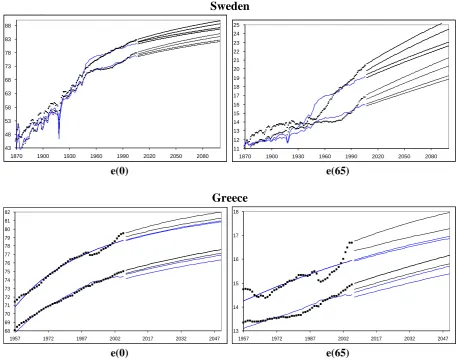
In our analysis, we obtain estimates of the period-based expected remaining lifetime,

e t

_x

( )

, by constructing a life table for each calendar year. In the general case, where the table is based on age grouping (called an abridged life table), under the assumption of the constant force of mortality (CFM), then for any (grouped) agex

and calendar yeartthe force of mortality is constant:

m

x c

( )

t



m

x

( )

t

for 0 c n, wherenis the width of

the age grouping, and

m

_x

( )

t



_n

m t

_x

( )

. The probability that an individual from age-groupx, in calendar yeart, does not reach the next age-group is n

q t

x

( )

 

1

exp



 

n

m

x

( )

t



. The hypothetical expected number of

persons alive at the start of each n-year age interval x, at calendar year t, is given by the iterative formula





( )

( )

1

( )

x n x n x

l

_

t



l t

 

q t

, with an arbitrary initial value

l t

₀

( )

, called the radix. The corresponding

number of person-years n x

( )

x

( )

1

n

( )



x n

( )

x

( )



a x

L t

n

l t

l

t

l t

n









_



_





 

_

_

_

 

_

_

_

_

_

_





_

_

_

, where





( )

1

( )

( )

( )

( )

n x

n x x

n

n x

q t

n

q t

t

a x

q t

m



_



  

_











is the average of the n-year period lived in the interval by those who died in that interval, under the CFM assumption. Therefore, the total future lifetime of the

l t

_x

( )

persons who attain age x, in calendar year t, is _x

( )

_{n i}

( )

i x

T t





_

L t

and the expected future remaining lifetime for

individuals from age-groupingxis ( ) ( ) ( )

x x

x T t e t

l t

 .

in the projected PCs. Starting from the observations

d

xt

we simulate

N

bootstrap samples {

( )i xt d

},

i=1,2,…,N

, where

d_xt( )i

are realizations from the Poisson distribution with parameters (

d

_xt

). For each

bootstrap sample, the GLM parameters B( )i are estimated and the associated PCs are projected on the basis of the dlr models selected from the original data. This yields Nrealizations for the expected remaining lifetimes and then the 95% CI are the percentile intervals

CI

95





p

0.025

,

p

0.975



, for each forecast year. The bootstrap confidence interval avoids the normal assumption and is more reliable than the standard normal interval (Efron and Tibshirani, 1998). The approach used corresponds to the semi-parametric bootstrap as described by Renshaw and Haberman (2008) and by Pitacco et al (2008).

3. Applications

3.1 The data

In order to illustrate the methodology, studies from two countries are conducted:  Sweden male-female mortality experience, calendar years 1751-2006  Greece male-female mortality experience, calendar years 1957-2006.

These countries have been selected because Sweden has the longest available mortality experience in contrast with the Greece mortality experience which is relatively short. The data are cross-classified by individual calendar year and age grouping ([0,5), [5,9),…,[95,



)) for Sweden and ([0,5), [5,9),…,[80, 85)) for Greece. Let [x]:=[x,x+5), for x=0,5,10,…. The data are freely provided, for Sweden by the “Human Mortality Database”(www.mortality.org) and for Greece by the General Secretariat of National Statistical Service of Greece (www.statistics.gr).

3.2 Optimal fitting period

We investigate model structures of the type _{1 1}

1

log ( ( )) ( ) ( )

k

j j

j

x

x t t L

   



 





, for each calendar year separately,

where L x_j1( ) denotes Legendre (zero-centered for j=2,…,k) orthonormal polynomials of degree j -1, for

j=1,2,…,k,and x the transformed values for the (grouped) ages, so that x [-1,1]. By monitoring the scaled deviance residuals in age and time effects, and examining the p-values of the associated statistical tests, the optimaldegree kfor Sweden males is found to be 15 and for females 14, and for Greece males and females the optimal degree is found to be 12. Especially for the case of Sweden, where the available data series is long, we find that these optimal degrees hold for different choices of investigation period.

Thus, each different period interval could produce different model identification and so different forecasts. For Sweden mortality data, we find that the optimum dlr model, for all the PCs, is the model with fixed slope and a random walk process for the level (i.e. an ARIMA(0,1,1) model plus constant). This kind of model satisfies the statistical criteria when testing the effect of changing the fitting periods. Although we could utilize all of the available historic mortality data, we can define a process of statistically determining the optimal fitting period, in respect of how well the log-central mortality rates would have been predicted if the model were used for different starting calendar years. We conduct an ex-post study for different starting calendar years: period(i,y)=[i; y], for i=1751,1752,…,y-20 (20 is the number of different age groups in order to apply PC analysis) and y=1971,1976,1981,1986,1991,1996,2001. For each y, the model performance is evaluated with the mean square error (MSE), of the observed log-central mortality rates and the projected log-central mortality rates, for all the ages. Thus, for fixedy, each starting yearigives a MSE value evaluated for all of the ages and all of the calendar years [y+1; 2006], which are of length 35,30,25,20,15,10,5 respectively for

y=1971,1976,1981,1986,1991,1996,2001. In order to combine the MSE values of the 7 different projected periods, we calculate the average values obtained for each starting calendar yeari, averaging over for differenty

values. This procedure will produce an average MSE value (AMSE) for each starting calendar yeari, from 1751 to 1951.

Figure 1 shows the AMSE for Sweden males and females, when the model structure consists of the first 3 most important interaction terms, and also, for comparison reasons, we demonstrate the AMSE results when the model structure consists of only the single most important interaction term. It is found that the optimum starting year, when utilizing the first 3 more important interaction terms, is 1869 for both males and females. In the case where we use only the 1stPC, for males the optimum starting year is 1857 and for females the minimum AMSE value is the last year (1951). However, in order to make long forecasts, we use as a starting year the calendar year 1809 where the AMSE exhibits a local minimum (very close to the value of 1951). Figure 1 shows these AMSE values. We note that for all of the starting calendar years, for both genders, the AMSE is lower when utilizing 3 or 4 interaction terms (PCs) rather than 1 interaction term (1 PC). That is, these ex-post investigations show that the method improves the forecasts for log-central mortality rates, when using more than 1 PC, as we would expect.

0,19 0,24 0,29 0,34 0,39

1750 1790 1830 1870 1910 1950

Males Males w ith 1PC

[image:14.595.146.475.442.621.2]

Females Females w ith 1PC

Figure 1: Average mean square error (AMSE) values vs. starting calendar year for Sweden

3.3 Residuals

Sweden Females

-3 -2 -1 0 1 2 3

- 20 40 60 80

-3 -2 -1 0 1 2 3

1869 1894 1919 1944 1969 1994

Sweden Males

-3 -2 -1 0 1 2 3

0 20 40 60 80

-3 -2 -1 0 1 2 3

1868 1898 1928 1958 1988

Greece Females

-4 -3 -2 -1 0 1 2 3

- 20 40 60 80 -4 -3 -2 -1 0 1 2 3

1957 1967 1977 1987 1997

Greece Males

-5 -4 -3 -2 -1 0 1 2 3 4 5

- 20 40 60 80 -5 -4 -3 -2 -1 0 1 2 3 4 5

[image:15.595.128.493.104.701.2]

1957 1967 1977 1987 1997

3.4 Model Components and Forecasts

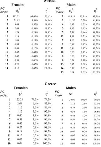
Table 1, gives the eigenvalues (



_i2-values)

based on

model structure (2), with the associated percentage variance and cumulative variance (

r

_i2-values) explained. After detecting the pattern of the



_i2 eigenvalues (scree plot) in association with the possible interpretations of the associated



_i

( )

x

and _i

( )

t

values, we retain, for the case of Sweden, 3 interaction terms (explaining 97,4% of the residual variation for males and 98,5% for females) and for Greece we keep 4 interaction terms (explaining the 96,6% of the residual variation for males and the 92,9% for females).

Figure 3 displays the most important components, with associated forecasts and CIs under the dlr structure, in significant order, for Sweden and Greece, based on model structure (2). For Sweden, for both genders, the most important interaction term,

v x

₁

( )

and



₁

( )

t

values, shows high values (in absolute tems) for the very young and for the very old ages: this explains the deviations (from the additive model) and trends for the very young (mainly for age groups [0]-[10]) in contrast with the very old (above age group [80[). The positive slope for the

1

( )

t



trend in association with negative (positive)

v x

₁

( )

values for the very young (old) ages indicates the relative improvement (deterioration) for these ages from the independent model. This term accounts for about 94% of the total residual variations. The 2ndmost important interaction term explains the deviations and trends mainly for the age groups [15]-[30], for both males and females. The



₂

( )

t

trend for these ages shows a relative deterioration from the independent model after the 1960s (negative slope after the 1960s in association with the negative

v x

₂

( )

values). This term explains about 3,3% and 2,2% of the females and males total residual variations respectively. This feature reproduces the well known “accident hump”, occurring at these ages

The 3rd most important interaction term (



₃

( )

t

and

v x

₃

( )

values) refers mainly to age groups [35],[40] for males, showing a relative improvement after the 1980s, and for females, it refers mainly to age groups [65]-[75] showing a relative improvement after the 1950s. It explains about 1,5% and 1,2% of the females and males residual variations respectively.

For Greece, the 1stinteraction term explains the deviations and trends for the very young (mainly for age groups [0]-[10]) in contrast with the very old for females only (above age group [75[). It explains about 79,3% and 90,3% of the females and males residual variations respectively. The 2ndmost important interaction term (



₃

( )

t

and

v x

₃

( )

values), for females, explains the relative improvement mainly for the age groups [65],[70] for the last few years, accounting for 6,6% of the total variations. For males, it explains the relative deterioration, from the independent model, mainly for the age groups [25]-[45] after the 1990s in contrast with the age groups [65]-[75], accounting for the 2,8% of the residual variations. The 3rd most important interaction term (



₂

( )

t

and

2

( )

v x

values), for both genders, refers mainly to age group [20]. This probably explains the “accident hump”, accounting for about 3,5% and 2% of the females and males residual variations respectively. We note that the other high

v x

₂

( )

(absolute) values have been accounted for and explained in the previous more significant interaction terms. Thus, we may conclude that, if we had used the PC variances, represented by the



_i

’s

values, instead of the

eigenvalues parameters



_i2, to define the number of interaction terms needed to be