E534 - B
IGD
ATAA
PPLICATIONSGeoffrey C. Fox Gregor von Laszewski
E534 - B
IGD
ATAA
PPLICATIONS1 PREFACE
1.1 Disclaimer ☁
1.1.1 Acknowledgment 1.1.2 Extensions
2 WEEK 1
2.1 Part I Motivation I ☁ 2.1.1 Motivation
2.1.2 00) Mechanics of Course, Summary, and overall remarks on course 2.1.2.1 01A) Technology Hypecycle I
2.1.2.2 01B) Technology Hypecycle II 2.1.2.3 01C) Technology Hypecycle III 2.1.2.4 01D) Technology Hypecycle IV 2.1.3 02)
2.1.3.1 02A) Clouds/Big Data Applications I 2.1.3.2 02B) Cloud/Big Data Applications II 2.1.3.3 02C) Cloud/Big Data
2.1.4 03) Jobs In areas like Data Science, Clouds and Computer Science and Computer
2.1.5 04) Industry, Technology, Consumer Trends Basic trends 2018 Lectures 4A 4B have
2.1.6 05) Digital Disruption and Transformation The Past displaced by Digital
2.1.7 06)
2.1.8 06A) Computing Model I Industry adopted clouds which are attractive for data
2.1.8.1 06B) Computing Model II with 3 subsections is removed; please see 2018
2.1.9 07) Research Model 4th Paradigm; From Theory to Data driven science?
2.1.10 08) Data Science Pipeline DIKW: Data, Information, Knowledge, Wisdom, Decisions.
2.1.11 09) Physics: Looking for Higgs Particle with Large Hadron Collider LHC Physics as a big data example
example
2.1.13 11) Recommender Systems II Exploring Data Bags and Spaces 2.1.14 12) Web Search and Information Retrieval Another Big Data Example
2.1.15 13) Cloud Applications in Research Removed Science Clouds, Internet of Things
2.1.16 14) Parallel Computing and MapReduce Software Ecosystems 2.1.17 15) Online education and data science education Removed. 2.1.18 16) Conclusions
3 WEEK 2
3.1 Part II Motivation Archive ☁
3.1.1 2018 BDAA Motivation-1A) Technology Hypecycle I 3.1.2 2018 BDAA Motivation-1B) Technology Hypecycle II
3.1.3 2018 BDAA Motivation-2B) Cloud/Big Data Applications II 3.1.4 2018 BDAA Motivation-4A) Industry Trends I
3.1.5 2018 BDAA Motivation-4B) Industry Trends II 3.1.6 2017 BDAA Motivation-4C)Industry Trends III 3.1.7 2018 BDAA Motivation-6B) Computing Model II
3.1.8 2017 BDAA Motivation-8) Data Science Pipeline DIKW
3.1.9 2017 BDAA Motivation-13) Cloud Applications in Research Science Clouds Internet of Things
3.1.10 2017 BDAA Motivation-15) Data Science Education Opportunities at Universities
4 WEEK 3
4.1 Part III Cloud ☁
4.1.1 A. Summary of Course 4.1.2 B. Defining Clouds I 4.1.3 C. Defining Clouds II
4.1.4 D. Defining Clouds III: Cloud Market Share 4.1.5 E. Virtualization: Virtualization Technologies, 4.1.6 F. Cloud Infrastructure I
4.1.7 G. Cloud Infrastructure II 4.1.8 H. Cloud Software:
4.1.9 I. Cloud Applications I: Clouds in science where area called 4.1.10 J. Cloud Applications II: Characterize Applications using NIST 4.1.11 K. Parallel Computing
Data SIMD SPMD
4.1.13 M. Storage: Cloud data 4.1.14 N. HPC and Clouds
4.1.15 O. Comparison of Data Analytics with Simulation: 4.1.16 P. The Future I
4.1.17 Q. other Issues II
4.1.18 R. The Future and other Issues III 5 WEEK 4
5.1 Physics with Big Data Applications ☁ 5.1.1 Unit 8:
5.1.1.1 8.1 - Looking for Higgs: 1. Particle and Counting Introduction 1
5.1.1.2 8.2 - Looking for Higgs: 2. Particle and Counting Introduction 2
5.1.1.3 8.3 - Looking for Higgs: 3. Particle Experiments
5.1.1.4 8.4 - Looking for Higgs: 4. Accelerator Picture Gallery of Big Science
5.1.2 Unit 9
5.1.2.1 9.1 - Looking for Higgs II: 1: Class Software 5.1.2.2 9.2 - Looking for Higgs II: 2: Event Counting
5.1.2.3 9.3 - Looking for Higgs II: 3: With Python examples of Signal plus Background
5.1.2.4 9.4 - Looking for Higgs II: 4: Change shape of background & number of Higgs Particles
5.1.3 Unit 10
5.1.3.1 10.1 - Statistics Overview and Fundamental Idea: Random Variables
5.1.3.2 10.2 - Physics and Random Variables I 5.1.3.3 10.3 - Physics and Random Variables II
5.1.3.4 10.4 - Statistics of Events with Normal Distributions 5.1.3.5 10.5 - Gaussian Distributions
5.1.3.6 10.6 - Using Statistics 5.1.4 Unit 11
5.1.4.5 11.5 - Monte Carlo Method 5.1.4.6 11.6 - Poisson Distribution 5.1.4.7 11.7 - Central Limit Theorem
5.1.4.8 11.8 - Interpretation of Probability: Bayes v. Frequency 6 WEEK 5
6.1 Google Colab ☁
6.1.1 Introduction to Google Colab 6.1.2 Programming in Google Colab
6.1.3 Benchamrking in Google Colab with Cloudmesh 7 WEEK 6
7.1 Introduction to Deep Learning ☁ 7.1.1 MNIST Classification Version 1 7.1.2 Using Cloudmesh Common 7.1.3 Import Libraries
7.1.4 Pre-process data 7.1.4.1 Load data
7.1.4.2 Identify Number of Classes
7.1.4.3 Convert Labels To One-Hot Vector 7.1.5 Image Reshaping
7.1.6 Resize and Normalize 7.1.7 Create a Keras Model 7.1.8 Compile and Train 7.1.9 Testing
7.1.10 Final Note 7.1.10.1 Reference: 8 WEEK 7
8.1 Sports with Big Data Applications ☁ 8.1.1 Unit 32
8.1.1.1 Lesson Summaries
8.1.2 BDAA 32.1 - E534 Sports - Introduction and Sabermetrics (Baseball Informatics) Lesson
8.1.2.1 BDAA 32.2 - E534 Sports - Basic Sabermetrics
8.1.2.2 BDAA 32.3 - E534 Sports - Wins Above Replacement 8.1.3 Unit 33
8.1.3.4 BDAA 33.4 - E534 Sports - Other Video Data Gathering in Baseball
8.1.4 Unit 34
8.1.4.1 BDAA 34.1 - E534 Sports - Wearables
8.1.4.2 BDAA 34.2 - E534 Sports - Soccer and the Olympics
8.1.4.3 BDAA 34.3 - E534 Sports - Spatial Visualization in NFL and NBA
8.1.4.4 BDAA 34.4 - E534 Sports - Tennis and Horse Racing 9 WEEK 8
9.1 Introduction to Deep Learning Part I ☁ 9.1.1 Intro Unit Summary
9.1.1.1 Optimization
9.1.1.2 First Deep Learning Example 9.1.1.3 Deep Learning Basics
9.1.1.4 Deep Learning Types 10 WEEK 9
10.1 Introduction to Deep Learning Part II: Applications ☁ 10.1.1 Recommender: Overview of Recommender Systems 10.1.2 Retail: Overview of AI in Retail Sector (e-commerce)
10.1.3 RideHailing: Overview of AI in Ride Hailing Industry (Uber, Lyft, Didi)
10.1.4 SelfDriving: Overview of AI in Self (AI-Assisted) Driving cars 10.1.5 Imaging: Overview of Scene Understanding
10.1.6 MainlyMedicine: Overview of AI in Health and Telecommunication
10.1.7 BankingFinance: Overview of Banking and Finance 11 ASSIGNMENTS
11.1 Assignments ☁
11.2 WEEKLY ASSIGNMENTS 11.2.1 Assignment 1 ☁
11.2.2 Assignment 2 ☁ 11.2.3 Assignment 3 ☁ 11.2.4 Assignment 4 ☁ 11.2.5 Assignment 5 ☁ 11.2.6 Assignment 6 ☁ 12 GITHUB
12.1.1 How to check this? 12.1.1.1 Step 1
12.1.1.2 Step 2 12.1.1.3 Step 3 12.1.1.4 Step 4
1 PREFACE
Mon Nov 4 19:04:12 EST 2019 ☁
1.1 D
ISCLAIMER☁
This book has been generated with Cyberaide Bookmanager.
Bookmanager is a tool to create a publication from a number of sources on the internet. It is especially useful to create customized books, lecture notes, or handouts. Content is best integrated in markdown format as it is very fast to produce the output.
Bookmanager has been developed based on our experience over the last 3 years with a more sophisticated approach. Bookmanager takes the lessons from this approach and distributes a tool that can easily be used by others.
The following shields provide some information about it. Feel free to click on them.
pypi
pypi v0.2.24v0.2.24 LicenseLicense Apache 2.0Apache 2.0 pythonpython 3.73.7 formatformat wheelwheel statusstatus stablestable buildbuild unknownunknown
1.1.1 Acknowledgment
If you use bookmanager to produce a document you must include the following acknowledgement.
“This document was produced with Cyberaide Bookmanager
developed by Gregor von Laszewski available at
https://pypi.python.org/pypi/cyberaide-bookmanager. It is in the responsibility of the user to make sure an author acknowledgement section is included in your document. Copyright verification of content included in a book is responsibility of the book editor.”
The bibtex entry is
1.1.2 Extensions
We are happy to discuss with you bugs, issues and ideas for enhancements. Please use the convenient github issues at
https://github.com/cyberaide/bookmanager/issues
Please do not file with us issues that relate to an editors book. They will provide you with their own mechanism on how to correct their content.
author = {Gregor von Laszewski}, title = {{Cyberaide Book Manager}}, howpublished = {pypi},
month = apr, year = 2019,
2.1 P
ARTI M
OTIVATIONI
☁
2.1.1 Motivation
Big Data Applications & Analytics: Motivation/Overview; Machine (actually Deep) Learning, Big Data, and the Cloud; Centerpieces of the Current and Future Economy,
2.1.2 00) Mechanics of Course, Summary, and overall remarks on
course
In this section we discuss the summary of the motivation section.
Video
2.1.2.1 01A) Technology Hypecycle I
Today clouds and big data have got through the hype cycle (they have emerged) but features like blockchain, serverless and machine learning are on recent hype cycles while areas like deep learning have several entries (as in fact do clouds) Gartner’s Hypecycles and especially that for emerging technologies in 2019 The phases of hypecycles Priority Matrix with benefits and adoption time Initial discussion of 2019 Hypecycle for Emerging Technologies
Video
2.1.2.2 01B) Technology Hypecycle II
but features like blockchain, serverless and machine learning are on recent hype cycles while areas like deep learning have several entries (as in fact do clouds) Gartner’s Hypecycles and especially that for emerging technologies in 2019 Details of 2019 Emerging Technology and related (AI, Cloud) Hypecycles
Video
2.1.2.3 01C) Technology Hypecycle III
Today clouds and big data have got through the hype cycle (they have emerged) but features like blockchain, serverless and machine learning are on recent hype cycles while areas like deep learning have several entries (as in fact do clouds) Gartners Hypecycles and Priority Matrices for emerging technologies in 2018, 2017 and 2016 More details on 2018 will be found in Unit 1A of 2018 Presentation and details of 2015 in Unit 1B (Journey to Digital Business). 1A in 2018 also discusses 2017 Data Center Infrastructure removed as this hype cycle disappeared in later years.
Video
2.1.2.4 01D) Technology Hypecycle IV
Video
2.1.3 02)
2.1.3.1 02A) Clouds/Big Data Applications I
The Data Deluge Big Data; a lot of the best examples have NOT been updated (as I can’t find updates) so some slides old but still make the correct points Big Data Deluge has become the Deep Learning Deluge Big Data is an agreed fact; Deep Learning still evolving fast but has stream of successes!
Video
2.1.3.2 02B) Cloud/Big Data Applications II
Clouds in science where area called cyberinfrastructure; The usage pattern from NIST is removed. See 2018 lectures 2B of the motivation for this discussion
Video
2.1.3.3 02C) Cloud/Big Data
Video
2.1.4 03) Jobs In areas like Data Science, Clouds and Computer
Science and Computer
Engineering
Video
2.1.5 04) Industry, Technology, Consumer Trends Basic trends
2018 Lectures 4A 4B have
more details removed as dated but still valid See 2018 Lesson 4C for 3 Technology trends for 2016: Voice as HCI, Cars, Deep Learning
Video
2.1.6 05) Digital Disruption and Transformation The Past
displaced by Digital
Disruption; some more details are in 2018 Presentation Lesson 5
2.1.7 06)
2.1.8 06A) Computing Model I Industry adopted clouds which are
attractive for data
analytics. Clouds are a dominant force in Industry. Examples are given
2.1.8.1 06B) Computing Model II with 3 subsections is removed; please see 2018
Presentation for this Developments after 2014 mainly from Gartner Cloud Market share Blockchain
Video
2.1.9 07) Research Model 4th Paradigm; From Theory to Data
driven science?
Video
2.1.10 08) Data Science Pipeline DIKW: Data, Information,
Knowledge, Wisdom, Decisions.
More details on Data Science Platforms are in 2018 Lesson 8 presentation
2.1.11 09) Physics: Looking for Higgs Particle with Large Hadron
Collider LHC Physics as a big data example
Video
2.1.12 10) Recommender Systems I General remarks and Netflix
example
Video
2.1.13 11) Recommender Systems II Exploring Data Bags and
Spaces
Video
2.1.14 12) Web Search and Information Retrieval Another Big
Data Example
Video
Part 12 continuation. See 2018 Presentation (same as 2017 for lesson 13) and Cloud Unit 2019-I) this year
Video
2.1.16 14) Parallel Computing and MapReduce Software
Ecosystems
Video
2.1.17 15) Online education and data science education Removed.
You can find it in the 2017 version. In Section 3.1 you can see more about this.
Video
2.1.18 16) Conclusions
Conclusion contain in the latter part of the part 15.
3.1 P
ARTII M
OTIVATIONA
RCHIVE☁
3.1.1 2018 BDAA Motivation-1A) Technology Hypecycle I
In this section we discuss on general remarks including Hype curves.
Video
3.1.2 2018 BDAA Motivation-1B) Technology Hypecycle II
In this section we continue our discussion on general remarks including Hype curves.
Video
3.1.3 2018 BDAA Motivation-2B) Cloud/Big Data Applications II
In this section we discuss clouds in science where area called cyberinfrastructure; the usage pattern from NIST Artificial Intelligence from Gartner and Meeker.
Video
3.1.4 2018 BDAA Motivation-4A) Industry Trends I
2014.
Video
3.1.5 2018 BDAA Motivation-4B) Industry Trends II
In this section we continue our discussion on industry trends. This section includes Lesson 4B 2015 onwards many technology adoption trends.
Video
3.1.6 2017 BDAA Motivation-4C)Industry Trends III
In this section we continue our discussion on industry trends. This section contains lesson 4C 2015 onwards 3 technology trends voice as HCI cars deep learning.
Video
3.1.7 2018 BDAA Motivation-6B) Computing Model II
Video
3.1.8 2017 BDAA Motivation-8) Data Science Pipeline DIKW
In this section, we discuss data science pipelines. This section also contains about data, information, knowledge, wisdom forming DIKW term. And also it contains some discussion on data science platforms.
Video
3.1.9 2017 BDAA Motivation-13) Cloud Applications in Research
Science Clouds Internet of Things
In this section we discuss about internet of things and related cloud applications.
Video
3.1.10 2017 BDAA Motivation-15) Data Science Education
Opportunities at Universities
In this section we discuss more on data science education opportunities.
4.1 P
ARTIII C
LOUD☁
4.1.1 A. Summary of Course
Video
4.1.2 B. Defining Clouds I
In this lecture we discuss the basic definition of cloud and two very simple examples of why virtualization is important.
Video
In this lecture we discuss how clouds are situated wrt HPC and supercomputers, why multicore chips are important in a typical data center.
4.1.3 C. Defining Clouds II
In this lecture we discuss service-oriented architectures, Software services as Message-linked computing capabilities.
Video
servers; serverless and microservices Gartner hypecycle and priority matrix on Infrastructure Strategies.
4.1.4 D. Defining Clouds III: Cloud Market Share
Video
In this lecture we discuss on how important the cloud market shares are and how much money do they make.
4.1.5 E. Virtualization: Virtualization Technologies,
Video
In this lecture we discuss hypervisors and the different approaches KVM, Xen, Docker and Openstack.
4.1.6 F. Cloud Infrastructure I
Video
In this lecture we comment on trends in the data center and its technologies. Clouds physically spread across the world Green computing Fraction of world’s computing ecosystem. In clouds and associated sizes an analysis from Cisco of size of cloud computing is discussed in this lecture.
Video
In this lecture, we discuss Gartner hypecycle and priority matrix on Compute Infrastructure Containers compared to virtual machines The emergence of artificial intelligence as a dominant force.
4.1.8 H. Cloud Software:
Video
In this lecture we discuss, HPC-ABDS with over 350 software packages and how to use each of 21 layers Google’s software innovations MapReduce in pictures Cloud and HPC software stacks compared Components need to support cloud/distributed system programming.
4.1.9 I. Cloud Applications I: Clouds in science where area called
Video
In this lecture we discuss cyberinfrastructure; the science usage pattern from NIST Artificial Intelligence from Gartner.
Video
In this lecture we discuss the approach Internet of Things with different types of MapReduce.
4.1.11 K. Parallel Computing
Video
In this lecture we discuss analogies, parallel computing in pictures and some useful analogies and principles.
4.1.12 L. Real Parallel Computing: Single Program/Instruction
Multiple Data SIMD SPMD
Video
In this lecture, we discuss Big Data and Simulations compared and we furthermore discusses what is hard to do.
4.1.13 M. Storage: Cloud data
In this lecture we discuss about the approaches, repositories, file systems, data lakes.
4.1.14 N. HPC and Clouds
Video
In this lecture we discuss the Branscomb Pyramid Supercomputers versus clouds Science Computing Environments.
4.1.15 O. Comparison of Data Analytics with Simulation:
Video
In this lecture we discuss the structure of different applications for simulations and Big Data Software implications Languages.
4.1.16 P. The Future I
Video
In this lecture we discuss Gartner cloud computing hypecycle and priority matrix 2017 and 2019 Hyperscale computing Serverless and FaaS Cloud Native Microservices Update to 2019 Hypecycle.
Video
In this lecture we discuss on Security Blockchain.
4.1.18 R. The Future and other Issues III
Video
5 WEEK 4
5.1 P
HYSICS WITHB
IGD
ATAA
PPLICATIONS☁
E534 2019 Big Data Applications and Analytics Discovery of Higgs Boson Part I (Unit 8) Section Units 9-11 Summary: This section starts by describing the LHC accelerator at CERN and evidence found by the experiments suggesting existence of a Higgs Boson. The huge number of authors on a paper, remarks on histograms and Feynman diagrams is followed by an accelerator picture gallery. The next unit is devoted to Python experiments looking at histograms of Higgs Boson production with various forms of shape of signal and various background and with various event totals. Then random variables and some simple principles of statistics are introduced with explanation as to why they are relevant to Physics counting experiments. The unit introduces Gaussian (normal) distributions and explains why they seen so often in natural phenomena. Several Python illustrations are given. Random Numbers with their Generators and Seeds lead to a discussion of Binomial and Poisson Distribution. Monte-Carlo and accept-reject methods. The Central Limit Theorem concludes discussion.
5.1.1 Unit 8:
5.1.1.1 8.1 - Looking for Higgs: 1. Particle and Counting Introduction 1
We return to particle case with slides used in introduction and stress that particles often manifested as bumps in histograms and those bumps need to be large enough to stand out from background in a statistically significant fashion.
5.1.1.2 8.2 - Looking for Higgs: 2. Particle and Counting Introduction 2
diagrams describe processes in a fundamental fashion.
5.1.1.3 8.3 - Looking for Higgs: 3. Particle Experiments
We give a few details on one LHC experiment ATLAS. Experimental physics papers have a staggering number of authors and quite big budgets. Feynman diagrams describe processes in a fundamental fashion
5.1.1.4 8.4 - Looking for Higgs: 4. Accelerator Picture Gallery of Big Science
This lesson gives a small picture gallery of accelerators. Accelerators, detection chambers and magnets in tunnels and a large underground laboratory used fpr experiments where you need to be shielded from background like cosmic rays.
5.1.2 Unit 9
This unit is devoted to Python experiments with Geoffrey looking at histograms of Higgs Boson production with various forms of shape of signal and various background and with various event totals
5.1.2.1 9.1 - Looking for Higgs II: 1: Class Software
for class
5.1.2.2 9.2 - Looking for Higgs II: 2: Event Counting
We define ‘’event counting’’ data collection environments. We discuss the python and Java code to generate events according to a particular scenario (the important idea of Monte Carlo data). Here a sloping background plus either a Higgs particle generated similarly to LHC observation or one observed with better resolution (smaller measurement error).
5.1.2.3 9.3 - Looking for Higgs II: 3: With Python examples of Signal plus Background
This uses Monte Carlo data both to generate data like the experimental observations and explore effect of changing amount of data and changing measurement resolution for Higgs.
5.1.2.4 9.4 - Looking for Higgs II: 4: Change shape of background & number of Higgs Particles
5.1.3 Unit 10
In this unit we discuss;
E534 2019 Big Data Applications and Analytics Discovery of Higgs Boson: Big Data Higgs Unit 10: Looking for Higgs Particles Part III: Random Variables, Physics and Normal Distributions Section Units 9-11 Summary: This section starts by describing the LHC accelerator at CERN and evidence found by the experiments suggesting existence of a Higgs Boson. The huge number of authors on a paper, remarks on histograms and Feynman diagrams is followed by an accelerator picture gallery. The next unit is devoted to Python experiments looking at histograms of Higgs Boson production with various forms of shape of signal and various background and with various event totals. Then random variables and some simple principles of statistics are introduced with explanation as to why they are relevant to Physics counting experiments. The unit introduces Gaussian (normal) distributions and explains why they seen so often in natural phenomena. Several Python illustrations are given. Random Numbers with their Generators and Seeds lead to a discussion of Binomial and Poisson Distribution. Monte-Carlo and accept-reject methods. The Central Limit Theorem concludes discussion. Big Data Higgs Unit 10: Looking for Higgs Particles Part III: Random Variables, Physics and Normal Distributions Overview: Geoffrey introduces random variables and some simple principles of statistics and explains why they are relevant to Physics counting experiments. The unit introduces Gaussian (normal) distributions and explains why they seen so often in natural phenomena. Several Python illustrations are given. Java is currently not available in this unit.
5.1.3.1 10.1 - Statistics Overview and Fundamental Idea: Random Variables
5.1.3.2 10.2 - Physics and Random Variables I
We describe the DIKW pipeline for the analysis of this type of physics experiment and go through details of analysis pipeline for the LHC ATLAS experiment. We give examples of event displays showing the final state particles seen in a few events. We illustrate how physicists decide whats going on with a plot of expected Higgs production experimental cross sections (probabilities) for signal and background.
5.1.3.3 10.3 - Physics and Random Variables II
We describe the DIKW pipeline for the analysis of this type of physics experiment and go through details of analysis pipeline for the LHC ATLAS experiment. We give examples of event displays showing the final state particles seen in a few events. We illustrate how physicists decide whats going on with a plot of expected Higgs production experimental cross sections (probabilities) for signal and background.
5.1.3.4 10.4 - Statistics of Events with Normal Distributions
5.1.3.5 10.5 - Gaussian Distributions
We introduce the Gaussian distribution and give Python examples of the fluctuations in counting Gaussian distributions.
5.1.3.6 10.6 - Using Statistics
We discuss the significance of a standard deviation and role of biases and insufficient statistics with a Python example in getting incorrect answers.
5.1.4 Unit 11
In this section we discuss;
phenomena. Several Python illustrations are given. Random Numbers with their Generators and Seeds lead to a discussion of Binomial and Poisson Distribution. Monte-Carlo and accept-reject methods. The Central Limit Theorem concludes discussion. Big Data Higgs Unit 11: Looking for Higgs Particles Part IV: Random Numbers, Distributions and Central Limit Theorem Unit Overview: Geoffrey discusses Random Numbers with their Generators and Seeds. It introduces Binomial and Poisson Distribution. Monte-Carlo and accept-reject methods are discussed. The Central Limit Theorem and Bayes law concludes discussion. Python and Java (for student - not reviewed in class) examples and Physics applications are given.
5.1.4.1 11.1 - Generators and Seeds I
We define random numbers and describe how to generate them on the computer giving Python examples. We define the seed used to define to specify how to start generation.
5.1.4.2 11.2 - Generators and Seeds II
We define random numbers and describe how to generate them on the computer giving Python examples. We define the seed used to define to specify how to start generation.
5.1.4.3 11.3 - Binomial Distribution
5.1.4.4 11.4 - Accept-Reject
We introduce an advanced method – accept/reject – for generating random variables with arbitrary distrubitions.
5.1.4.5 11.5 - Monte Carlo Method
We define Monte Carlo method which usually uses accept/reject method in typical case for distribution.
5.1.4.6 11.6 - Poisson Distribution
We extend the Binomial to the Poisson distribution and give a set of amusing examples from Wikipedia.
5.1.4.7 11.7 - Central Limit Theorem
5.1.4.8 11.8 - Interpretation of Probability: Bayes v. Frequency
6 WEEK 5
6.1 G
OOGLEC
OLAB☁
In this section we are going to introduce you, how to use Google Colab to run deep learning models.
6.1.1 Introduction to Google Colab
This video contains the introduction to Google Colab. In this section we will be learning how to start a Google Colab project.
6.1.2 Programming in Google Colab
In this video we will learn how to create a simple, Colab Notebook. Required Installations
6.1.3 Benchamrking in Google Colab with Cloudmesh
In this video we learn how to do a basic benchmark with Cloudmesh tools. Cloudmesh StopWatch will be used in this tutorial.
Required Installations
pip install numpy
pip install numpy
7 WEEK 6
7.1 I
NTRODUCTION TOD
EEPL
EARNING☁
In this tutorial we will learn the fist lab on deep neural networks. Basic classification using deep learning will be discussed in this chapter.
7.1.1 MNIST Classification Version 1
7.1.2 Using Cloudmesh Common
Here we do a simple benchmark. We calculate compile time, train time, test time and data loading time for this example. Installing cloudmesh-common library is the first step. Focus on this section because the ** Assignment 4 ** will be focused on the content of this lab.
!pip install cloudmesh-common
Collecting cloudmesh-common
[?25l Downloading https://files.pythonhosted.org/packages/42/72/3c4aabce294273db9819be4a0a350f506d2b50c19b7177fb6cfe1cbbfe63/cloudmesh_common-4.2.13-py2.py3-none-any.whl (55kB) [K |████████████████████████████████| 61kB 4.1MB/s
[?25hRequirement already satisfied: future in /usr/local/lib/python3.6/dist-packages (from cloudmesh-common) (0.16.0)
Collecting pathlib2 (from cloudmesh-common)
Downloading https://files.pythonhosted.org/packages/e9/45/9c82d3666af4ef9f221cbb954e1d77ddbb513faf552aea6df5f37f1a4859/pathlib2-2.3.5-py2.py3-none-any.whl Requirement already satisfied: python-dateutil in /usr/local/lib/python3.6/dist-packages (from cloudmesh-common) (2.5.3)
Collecting simplejson (from cloudmesh-common)
[?25l Downloading https://files.pythonhosted.org/packages/e3/24/c35fb1c1c315fc0fffe61ea00d3f88e85469004713dab488dee4f35b0aff/simplejson-3.16.0.tar.gz (81kB) [K |████████████████████████████████| 81kB 10.6MB/s
[?25hCollecting python-hostlist (from cloudmesh-common)
Downloading https://files.pythonhosted.org/packages/3d/0f/1846a7a0bdd5d890b6c07f34be89d1571a6addbe59efe59b7b0777e44924/python-hostlist-1.18.tar.gz Requirement already satisfied: pathlib in /usr/local/lib/python3.6/dist-packages (from cloudmesh-common) (1.0.1)
Collecting colorama (from cloudmesh-common)
Downloading https://files.pythonhosted.org/packages/4f/a6/728666f39bfff1719fc94c481890b2106837da9318031f71a8424b662e12/colorama-0.4.1-py2.py3-none-any.whl Collecting oyaml (from cloudmesh-common)
Downloading https://files.pythonhosted.org/packages/00/37/ec89398d3163f8f63d892328730e04b3a10927e3780af25baf1ec74f880f/oyaml-0.9-py2.py3-none-any.whl Requirement already satisfied: humanize in /usr/local/lib/python3.6/dist-packages (from cloudmesh-common) (0.5.1)
Requirement already satisfied: psutil in /usr/local/lib/python3.6/dist-packages (from cloudmesh-common) (5.4.8)
Requirement already satisfied: six in /usr/local/lib/python3.6/dist-packages (from pathlib2->cloudmesh-common) (1.12.0)
Requirement already satisfied: pyyaml in /usr/local/lib/python3.6/dist-packages (from oyaml->cloudmesh-common) (3.13)
Building wheels for collected packages: simplejson, python-hostlist Building wheel for simplejson (setup.py) ... [?25l[?25hdone
In this lesson we discuss in how to create a simple IPython Notebook to solve an image classification problem. MNIST contains a set of pictures
7.1.3 Import Libraries
Note: https://python-future.org/quickstart.html
Stored in directory: /root/.cache/pip/wheels/5d/1a/1e/0350bb3df3e74215cd91325344cc86c2c691f5306eb4d22c77 Building wheel for python-hostlist (setup.py) ... [?25l[?25hdone
Created wheel for python-hostlist: filename=python_hostlist-1.18-cp36-none-any.whl size=38517 sha256=71fbb29433b52fab625e17ef2038476b910bc80b29a822ed00a783d3b1fb73e4 Stored in directory: /root/.cache/pip/wheels/56/db/1d/b28216dccd982a983d8da66572c497d6a2e485eba7c4d6cba3
Successfully built simplejson python-hostlist
Installing collected packages: pathlib2, simplejson, python-hostlist, colorama, oyaml, cloudmesh-common
Successfully installed cloudmesh-common-4.2.13 colorama-0.4.1 oyaml-0.9 pathlib2-2.3.5 python-hostlist-1.18 simplejson-3.16.0
! python3 --version
Python 3.6.8
! pip install tensorflow-gpu==1.14.0
Collecting tensorflow-gpu==1.14.0
[?25l Downloading https://files.pythonhosted.org/packages/76/04/43153bfdfcf6c9a4c38ecdb971ca9a75b9a791bb69a764d652c359aca504/tensorflow_gpu-1.14.0-cp36-cp36m-manylinux1_x86_64.whl (377.0MB) [K |████████████████████████████████| 377.0MB 77kB/s
[?25hRequirement already satisfied: six>=1.10.0 in /usr/local/lib/python3.6/dist-packages (from tensorflow-gpu==1.14.0) (
Requirement already satisfied: grpcio>=1.8.6 in /usr/local/lib/python3.6/dist-packages (from tensorflow-gpu==1.14.0) (1.15.0 Requirement already satisfied: protobuf>=3.6.1 in /usr/local/lib/python3.6/dist-packages (from tensorflow-gpu==1.14.0) (3.7.1 Requirement already satisfied: keras-applications>=1.0.6 in /usr/local/lib/python3.6/dist-packages (from tensorflow-gpu==1.14.0) Requirement already satisfied: gast>=0.2.0 in /usr/local/lib/python3.6/dist-packages (from tensorflow-gpu==1.14.0) (0.2.2 Requirement already satisfied: astor>=0.6.0 in /usr/local/lib/python3.6/dist-packages (from tensorflow-gpu==1.14.0) (0.8.0 Requirement already satisfied: absl-py>=0.7.0 in /usr/local/lib/python3.6/dist-packages (from tensorflow-gpu==1.14.0) (0.8.0 Requirement already satisfied: wrapt>=1.11.1 in /usr/local/lib/python3.6/dist-packages (from tensorflow-gpu==1.14.0) (1.11.2 Requirement already satisfied: wheel>=0.26 in /usr/local/lib/python3.6/dist-packages (from tensorflow-gpu==1.14.0) (0.33.6
Requirement already satisfied: tensorflow-estimator<1.15.0rc0,>=1.14.0rc0 in /usr/local/lib/python3.6/dist-packages (from tensorflow-gpu==1.14.0) Requirement already satisfied: tensorboard<1.15.0,>=1.14.0 in /usr/local/lib/python3.6/dist-packages (from tensorflow-gpu==1.14.0)
Requirement already satisfied: numpy<2.0,>=1.14.5 in /usr/local/lib/python3.6/dist-packages (from tensorflow-gpu==1.14.0) Requirement already satisfied: termcolor>=1.1.0 in /usr/local/lib/python3.6/dist-packages (from tensorflow-gpu==1.14.0) (
Requirement already satisfied: keras-preprocessing>=1.0.5 in /usr/local/lib/python3.6/dist-packages (from tensorflow-gpu==1.14.0) Requirement already satisfied: google-pasta>=0.1.6 in /usr/local/lib/python3.6/dist-packages (from tensorflow-gpu==1.14.0) Requirement already satisfied: setuptools in /usr/local/lib/python3.6/dist-packages (from protobuf>=3.6.1->tensorflow-gpu==1.14.0) Requirement already satisfied: h5py in /usr/local/lib/python3.6/dist-packages (from keras-applications>=1.0.6->tensorflow-gpu==1.14.0) Requirement already satisfied: markdown>=2.6.8 in /usr/local/lib/python3.6/dist-packages (from tensorboard<1.15.0,>
=1.14.0-Requirement already satisfied: werkzeug>=0.11.15 in /usr/local/lib/python3.6/dist-packages (from tensorboard<1.15.0,> =1.14.0-Installing collected packages: tensorflow-gpu
Successfully installed tensorflow-gpu-1.14.0
from __future__ import absolute_import from __future__ import division from __future__ import print_function
import time
import numpy as np
from keras.models import Sequential
from keras.layers import Dense, Activation, Dropout from keras.utils import to_categorical, plot_model from keras.datasets import mnist
from cloudmesh.common.StopWatch import StopWatch
7.1.4 Pre-process data
7.1.4.1 Load data
First we load the data from the inbuilt mnist dataset from Keras
7.1.4.2 Identify Number of Classes
As this is a number classification problem. We need to know how many classes are there. So we’ll count the number of unique labels.
7.1.4.3 Convert Labels To One-Hot Vector
|Exercise MNIST_V1.0.0: Understand what is an one-hot vector?
7.1.5 Image Reshaping
The training model is designed by considering the data as a vector. This is a model dependent modification. Here we assume the image is a squared shape image.
7.1.6 Resize and Normalize
The next step is to continue the reshaping to a fit into a vector and normalize the
StopWatch.start("data-load")
(x_train, y_train), (x_test, y_test) = mnist.load_data() StopWatch.stop("data-load")
Downloading data from https://s3.amazonaws.com/img-datasets/mnist.npz 11493376/11490434 [==============================] - 1s 0us/step
num_labels = len(np.unique(y_train))
y_train = to_categorical(y_train) y_test = to_categorical(y_test)
data. Image values are from 0 - 255, so an easy way to normalize is to divide by the maximum value.
|Execrcise MNIST_V1.0.1: Suggest another way to normalize the data preserving the accuracy or improving the accuracy.
7.1.7 Create a Keras Model
Keras is a neural network library. Most important thing with Keras is the way we design the neural network.
In this model we have a couple of ideas to understand.
|Exercise MNIST_V1.1.0: Find out what is a dense layer?
A simple model can be initiated by using an Sequential instance in Keras. For this instance we add a single layer.
1. Dense Layer
2. Activation Layer (Softmax is the activation function)
Dense layer and the layer followed by it is fully connected. For instance the number of hidden units used here is 64 and the following layer is a dense layer followed by an activation layer.
|Execrcise MNIST_V1.2.0: Find out what is the use of an activation function. Find out why, softmax was used as the last layer.
x_train = np.reshape(x_train, [-1, input_size]) x_train = x_train.astype('float32') /255
x_test = np.reshape(x_test, [-1, input_size]) x_test = x_test.astype('float32') / 255
batch_size = 4
hidden_units =64
model = Sequential()
model.add(Dense(hidden_units, input_dim=input_size)) model.add(Dense(num_labels))
model.add(Activation('softmax')) model.summary()
images
7.1.8 Compile and Train
A keras model need to be compiled before it can be used to train the model. In
WARNING:tensorflow:From /usr/local/lib/python3.6/dist-packages/keras/backend/tensorflow_backend.py:66: The name tf.get_default_graph is deprecated. Please use tf.compat.v1.get_default_graph instead.
WARNING:tensorflow:From /usr/local/lib/python3.6/dist-packages/keras/backend/tensorflow_backend.py:541: The name tf.placeholder is deprecated. Please use tf.compat.v1.placeholder instead.
WARNING:tensorflow:From /usr/local/lib/python3.6/dist-packages/keras/backend/tensorflow_backend.py:4432: The name tf.random_uniform is deprecated. Please use tf.random.uniform instead.
Model: "sequential_1"
_________________________________________________________________ Layer (type) Output Shape Param # ================================================================= dense_1 (Dense) (None, 64) 50240 _________________________________________________________________ dense_2 (Dense) (None, 10) 650 _________________________________________________________________ activation_1 (Activation) (None, 10) 0
================================================================= Total params: 50,890
Trainable params: 50,890 Non-trainable params: 0
the compile function, you can provide the optimization that you want to add, metrics you expect and the type of loss function you need to use.
Here we use the adam optimizer, a famous optimizer used in neural networks.
Exercise MNIST_V1.3.0: Find 3 other optimizers used on neural networks.
The loss funtion we have used is the categorical_crossentropy.
Exercise MNIST_V1.4.0: Find other loss functions provided in keras. Your answer can limit to 1 or more.
Once the model is compiled, then the fit function is called upon passing the number of epochs, traing data and batch size.
The batch size determines the number of elements used per minibatch in optimizing the function.
Note: Change the number of epochs, batch size and see what happens.
Exercise MNIST_V1.5.0: Figure out a way to plot the loss function value. You can use any method you like.
7.1.9 Testing
Now we can test the trained model. Use the evaluate function by passing test data and batch size and the accuracy and the loss value can be retrieved.
StopWatch.start("compile")
model.compile(loss='categorical_crossentropy', optimizer='adam',
metrics=['accuracy']) StopWatch.stop("compile")
StopWatch.start("train")
model.fit(x_train, y_train, epochs=1, batch_size=batch_size) StopWatch.stop("train")
WARNING:tensorflow:From /usr/local/lib/python3.6/dist-packages/keras/optimizers.py:793: The name tf.train.Optimizer is deprecated. Please use tf.compat.v1.train.Optimizer instead.
WARNING:tensorflow:From /usr/local/lib/python3.6/dist-packages/keras/backend/tensorflow_backend.py:3576: The name tf.log is deprecated. Please use tf.math.log instead.
WARNING:tensorflow:From /usr/local/lib/python3.6/dist-packages/tensorflow/python/ops/math_grad.py:1250: add_dispatch_support. Instructions for updating:
Use tf.where in 2.0, which has the same broadcast rule as np.where
WARNING:tensorflow:From /usr/local/lib/python3.6/dist-packages/keras/backend/tensorflow_backend.py:1033: The name tf.assign_add is deprecated. Please use tf.compat.v1.assign_add instead.
Epoch 1/1
Exercise MNIST_V1.6.0: Try to optimize the network by changing the number of epochs, batch size and record the best accuracy that you can gain
7.1.10 Final Note
StopWatch.start("test")loss, acc = model.evaluate(x_test, y_test, batch_size=batch_size) print("\nTest accuracy: %.1f%%"% (100.0 * acc))
StopWatch.stop("test")
10000/10000 [==============================] - 1s 138us/step
Test accuracy: 91.0%
StopWatch.benchmark()
+---+---+
| Machine Attribute | Value |
+---+---+
| BUG_REPORT_URL | "https://bugs.launchpad.net/ubuntu/" | | DISTRIB_CODENAME | bionic | | DISTRIB_DESCRIPTION | "Ubuntu 18.04.3 LTS" | | DISTRIB_ID | Ubuntu | | DISTRIB_RELEASE | 18.04 | | HOME_URL | "https://www.ubuntu.com/" | | ID | ubuntu | | ID_LIKE | debian | | NAME | "Ubuntu" | | PRETTY_NAME | "Ubuntu 18.04.3 LTS" | | PRIVACY_POLICY_URL | "https://www.ubuntu.com/legal/terms-and-policies/privacy-policy"| | SUPPORT_URL | "https://help.ubuntu.com/" | | UBUNTU_CODENAME | bionic | | VERSION | "18.04.3 LTS (Bionic Beaver)" | | VERSION_CODENAME | bionic | | VERSION_ID | "18.04" | | cpu_count | 2 | | mac_version | | | machine | ('x86_64',) | | mem_active | 973.8 MiB | | mem_available | 11.7 GiB | | mem_free | 5.1 GiB | | mem_inactive | 6.3 GiB | | mem_percent | 8.3% | | mem_total | 12.7 GiB | | mem_used | 877.3 MiB | | node | ('8281485b0a16',) | | platform | Linux-4.14.137+-x86_64-with-Ubuntu-18.04-bionic | | processor | ('x86_64',) | | processors | Linux | | python | 3.6.8 (default, Jan 14 2019, 11:02:34) | | | [GCC 8.0.1 20180414 (experimental) [trunk revision 259383]] | | release | ('4.14.137+',) | | sys | linux | | system | Linux | | user | | | version | #1 SMP Thu Aug 8 02:47:02 PDT 2019 |
| win_version | |
+---+---+
+---+---+---+---+---+---+---+---+---+
| timer | time | start | tag | node | user | system | mac_version | win_version |
+---+---+---+---+---+---+---+---+---+
| data-load | 1.335 | 2019-09-27 13:37:41 | | ('8281485b0a16',) | | Linux | | | | compile | 0.047 | 2019-09-27 13:37:43 | | ('8281485b0a16',) | | Linux | | | | train | 20.58 | 2019-09-27 13:37:43 | | ('8281485b0a16',) | | Linux | | | | test | 1.393 | 2019-09-27 13:38:03 | | ('8281485b0a16',) | | Linux | | |
+---+---+---+---+---+---+---+---+---+
timer,time,starttag,node,user,system,mac_version,win_version data-load,1.335,None,('8281485b0a16',),,Linux,,
This programme can be defined as a hello world programme in deep learning. Objective of this exercise is not to teach you the depths of deep learning. But to teach you basic concepts that may need to design a simple network to solve a problem. Before running the whole code, read all the instructions before a code section. Solve all the problems noted in bold text with Exercise keyword (Exercise MNIST_V1.0 - MNIST_V1.6). Write your answers and submit a PDF by following the Assignment 5. Include codes or observations you made on those sections.
7.1.10.1 Reference:
Mnist Database
8 WEEK 7
8.1 S
PORTS WITHB
IGD
ATAA
PPLICATIONS☁
E534 2019 Big Data Applications and Analytics Sports Informatics Part I (Unit 32) Section Summary (Parts I, II, III): Sports sees significant growth in analytics with pervasive statistics shifting to more sophisticated measures. We start with baseball as game is built around segments dominated by individuals where detailed (video/image) achievement measures including PITCHf/x and FIELDf/x are moving field into big data arena. There are interesting relationships between the economics of sports and big data analytics. We look at Wearables and consumer sports/recreation. The importance of spatial visualization is discussed. We look at other Sports: Soccer, Olympics, NFL Football, Basketball, Tennis and Horse Racing.
8.1.1 Unit 32
Unit Summary (PartI, Unit 32): This unit discusses baseball starting with the movie Moneyball and the 2002-2003 Oakland Athletics. Unlike sports like basketball and soccer, most baseball action is built around individuals often interacting in pairs. This is much easier to quantify than many player phenomena in other sports. We discuss Performance-Dollar relationship including new stadiums and media/advertising. We look at classic baseball averages and sophisticated measures like Wins Above Replacement.
8.1.1.1 Lesson Summaries
8.1.2 BDAA 32.1 - E534 Sports - Introduction and Sabermetrics
(Baseball Informatics) Lesson
8.1.2.1 BDAA 32.2 - E534 Sports - Basic Sabermetrics
Different Types of Baseball Data, Sabermetrics, Overview of all data, Details of some statistics based on basic data, OPS, wOBA, ERA, ERC, FIP, UZR.
8.1.2.2 BDAA 32.3 - E534 Sports - Wins Above Replacement
Wins above Replacement WAR, Discussion of Calculation, Examples, Comparisons of different methods, Coefficient of Determination, Another, Sabermetrics Example, Summary of Sabermetrics.
8.1.3 Unit 33
E534 2019 Big Data Applications and Analytics Sports Informatics Part II (Unit 33) Section Summary (Parts I, II, III): Sports sees significant growth in analytics with pervasive statistics shifting to more sophisticated measures. We start with baseball as game is built around segments dominated by individuals where detailed (video/image) achievement measures including PITCHf/x and FIELDf/x are moving field into big data arena. There are interesting relationships between the economics of sports and big data analytics. We look at Wearables and consumer sports/recreation. The importance of spatial visualization is discussed. We look at other Sports: Soccer, Olympics, NFL Football, Basketball, Tennis and Horse Racing.
covering advances possible from using video from PITCHf/X, FIELDf/X, HITf/X, COMMANDf/X and MLBAM.
8.1.3.1 BDAA 33.1 - E534 Sports - Pitching Clustering
A Big Data Pitcher Clustering method introduced by Vince Gennaro, Data from Blog and video at 2013 SABR conference
8.1.3.2 BDAA 33.2 - E534 Sports - Pitcher Quality
Results of optimizing match ups, Data from video at 2013 SABR conference.
8.1.3.3 BDAA 33.3 - E534 Sports - PITCHf/X
Examples of use of PITCHf/X.
8.1.3.4 BDAA 33.4 - E534 Sports - Other Video Data Gathering in Baseball
FIELDf/X, MLBAM, HITf/X, COMMANDf/X.
E534 2019 Big Data Applications and Analytics Sports Informatics Part III (Unit 34). Section Summary (Parts I, II, III): Sports sees significant growth in analytics with pervasive statistics shifting to more sophisticated measures. We start with baseball as game is built around segments dominated by individuals where detailed (video/image) achievement measures including PITCHf/x and FIELDf/x are moving field into big data arena. There are interesting relationships between the economics of sports and big data analytics. We look at Wearables and consumer sports/recreation. The importance of spatial visualization is discussed. We look at other Sports: Soccer, Olympics, NFL Football, Basketball, Tennis and Horse Racing.
Unit Summary (Part III, Unit 34): We look at Wearables and consumer sports/recreation. The importance of spatial visualization is discussed. We look at other Sports: Soccer, Olympics, NFL Football, Basketball, Tennis and Horse Racing.
Lesson Summaries
8.1.4.1 BDAA 34.1 - E534 Sports - Wearables
Consumer Sports, Stake Holders, and Multiple Factors.
8.1.4.2 BDAA 34.2 - E534 Sports - Soccer and the Olympics
Soccer, Tracking Players and Balls, Olympics.
8.1.4.3 BDAA 34.3 - E534 Sports - Spatial Visualization in NFL and NBA
8.1.4.4 BDAA 34.4 - E534 Sports - Tennis and Horse Racing
9.1 I
NTRODUCTION TOD
EEPL
EARNINGP
ARTI
☁
E534 2019 BDAA DL Section Intro Unit: E534 2019 Big Data Applications and Analytics Introduction to Deep Learning Part I (Unit Intro) Section Summary This section covers the growing importance of the use of Deep Learning in Big Data Applications and Analytics. The Intro Unit is an introduction to the technology with examples incidental. It includes an introducton to the laboratory where we use Keras and Tensorflow. The Tech unit covers the deep learning technology in more detail. The Application Units cover deep learning applications at different levels of sophistication.
9.1.1 Intro Unit Summary
This unit is an introduction to deep learning with four major lessons
9.1.1.1 Optimization
Lesson Summaries Optimization: Overview of Optimization Opt lesson overviews optimization with a focus on issues of importance for deep learning. Gives a quick review of Objective Function, Local Minima (Optima), Annealing, Everything is an optimization problem with examples, Examples of Objective Functions, Greedy Algorithms, Distances in funny spaces, Discrete or Continuous Parameters, Genetic Algorithms, Heuristics.
Slides
9.1.1.2 First Deep Learning Example
identification of numbers from NIST database using a Multilayer Perceptron using Keras+Tensorflow running on Google Colab
Slides
9.1.1.3 Deep Learning Basics
DLBasic: Basic Terms Used in Deep Learning DLBasic lesson reviews important Deep Learning topics including Activation: (ReLU, Sigmoid, Tanh, Softmax), Loss Function, Optimizer, Stochastic Gradient Descent, Back Propagation, One-hot Vector, Vanishing Gradient, Hyperparameter
Slides
9.1.1.4 Deep Learning Types
10.1 I
NTRODUCTION TOD
EEPL
EARNINGP
ARTII:
A
PPLICATIONS☁
This section covers the growing importance of the use of Deep Learning in Big Data Applications and Analytics. The Intro Unit is an introduction to the technology with examples incidental. The MNIST Unit covers an example on Google Colaboratory. The Technology Unit covers deep learning approaches in more detail than the Intro Unit. The Tech Unit covers the deep learning technology in more detail. The Application Unit cover deep learning applications at different levels of sophistication.
Applications of Deep Learning Unit Summary This unit is an introduction to deep learning with currently 7 lessons
10.1.1 Recommender: Overview of Recommender Systems
Recommender engines used to be dominated by collaborative filtering using matrix factorization and k’th nearest neighbor approaches. Large systems like YouTube and Netflix now use deep learning. We look at sysyems like Spotify that use multiple sources of information.
Slides
10.1.2 Retail: Overview of AI in Retail Sector (e-commerce)
Slides
10.1.3 RideHailing: Overview of AI in Ride Hailing Industry
(Uber, Lyft, Didi)
The Ride Hailing industry will grow as it becomes main mobility method for many customers. Their technology investment includes deep learning for matching drivers and passengers. There is huge overlap with larger area of AI in transportation.
Slides
10.1.4 SelfDriving: Overview of AI in Self (AI-Assisted) Driving
cars
Automobile Industry needs to remake itself as mobility companies. Basic automotive industry flat to down but AI can improve productivity. Lesson also discusses electric vehicles and drones
Slides
10.1.5 Imaging: Overview of Scene Understanding
Slides
10.1.6 MainlyMedicine: Overview of AI in Health and
Telecommunication
Telecommunication Industry has little traditional growth to look forward to. It can use AI in its operation and exploit trove of Big Data it possesses. Medicine has many breakthrough opportunities but progress hard – partly due to data privacy restrictions. Traditional Bioinformatics areas progress but slowly; pathology is based on imagery and making much better progress with deep learning
Slides
10.1.7 BankingFinance: Overview of Banking and Finance
This FinTech sector has huge investments (larger than other applications we studied)and we can expect all aspects of Banking and Finance to be remade with online digital Banking as a Service. It is doubtful that traditional banks will thrive
11 ASSIGNMENTS
11.1 A
SSIGNMENTS☁
Due dates are on Canvas. Click on the links to checkout the assignment pages.
11.2 WEEKLY ASSIGNMENTS
11.2.1 Assignment 1
☁
In the first assignment you will be writing a technical document on the current technology trends that you’re pursuing and the trends that you would like to follow. In addition to this include some information about your background in programming and some projects that you have done. There is no strict format for this one, but we expect 2 page written document. Please submit a PDF.
Go to Canvas
11.2.2 Assignment 2
☁
In the second assignment, you will be working on Week 1 (see Section 2.1) lecture videos. Objectives are as follows.
1. Summarize what you have understood. (2 page)
2. Select a subtopic that you are interested in and research on the current trends (1 page)
3. Suggest ideas that could improve the existing work (imaginations and possibilities) (1 page)
Go to Canvas
11.2.3 Assignment 3
☁
In the third assignment, you will be working on (see Section 4.1) lecture videos. Objectives are as follows.
1. Summarize what you have understood. (2 page)
2. Select a subtopic that you are interested in and research on the current trends (1 page)
3. Suggest ideas that could improve the existing work (imaginations and possibilities) (1 page)
For this assignment we expect a 4 page document. You can use a single column format for this document. Make sure you write exactly 4 pages. For your research section make sure you add citations to the sections that you are going to refer. If you have issues in how to do citations you can reach a TA to learn how to do that. We will try to include some chapters on how to do this in our handbook. Submissions are in pdf format only.
Go to Canvas
11.2.4 Assignment 4
☁
In the fourth assignment, you will be working on (see Section 5.1) lecture videos. Objectives are as follows.
1. Summarize what you have understood. (1 page)
2. Select a subtopic that you are interested in and research on the current trends (0.5 page)
3. Suggest ideas that could improve the existing work (imaginations and possibilities) (0.5 page)
4. Summarize a specific video segment in the video lectures. To do this you need to follow these guidelines. Mention the video lecture name and section identification number. And also specify which range of minutes you have focused on the specific video lecture (2 pages).
format for this document. Make sure you write exactly 4 pages. For your research section make sure you add citations to the sections that you are going to refer. If you have issues in how to do citations you can reach a TA to learn how to do that. We will try to include some chapters on how to do this in our handbook. Submissions are in pdf format only.
Go to Canvas
11.2.5 Assignment 5
☁
In the fifth assignment, you will be working on (see Section 7.1) lecture videos. Objectives are as follows.
Run the given sample code and try to answer the questions under the exercise tag.
Follow the Exercises labelled from MNIST_V1.0.0 - MNIST_V1.6.0
For this assignment all you have to do is just answer all the questions. You can use a single column format for this document. Submissions are in pdf format only.
Go to Canvas
11.2.6 Assignment 6
☁
In the sixth assignment, you will be working on (see Section 8.1) lecture videos. Objectives are as follows.
1. Summarize what you have understood. (1 page)
2. Select a subtopic that you are interested in and research on the current trends (0.5 page)
3. Suggest ideas that could improve the existing work (imaginations and possibilities) (0.5 page)
5. Pick a sport you like and show case how it can be used with Big Data in order to improve the game (1 page). Use techniques used in the lecture videos and mention which lecture video refers to this technique.
For this assignment we expect a 5-page document. You can use a single column format for this document. Make sure you write exactly 5pages. For your research section make sure you add citations to the sections that you are going to refer. If you have issues in how to do citations you can reach a TA to learn how to do that. We will try to include some chapters on how to do this in our handbook. Submissions are in pdf format only.
12 GITHUB
12.1 T
RACKP
ROGRESS WITHG
ITHUB☁
We will be adding git issues for all the assignments provided in the class. This way you can also keep a track on the items need to be completed. It is like a todo list. You can check things once you complete it. This way you can easily track what you need to do and you can comment on the issue to report the questions you have. This is an experimental idea we are trying in the class. Hope this helps to manage your work load efficiently.
12.1.1 How to check this?
All you have to do is go to your git repository. Here are the steps to use this tool effectively.
12.1.1.1 Step 1
Go to the repo. Here we use a sample repo.
Sample Repo
Link to your repo will be https://github.com/cloudmesh-community/fa19-{class-id}-{hid}
class-id is your class number for instance 534. hid is your homework id assigned.
12.1.1.2 Step 2
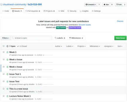
Figure 1: Git Repo View
12.1.1.3 Step 3
Figure 2: Git Issue List
12.1.1.4 Step 4
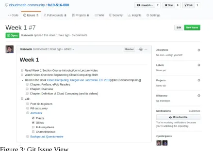
Figure 3: Git Issue View
In here you will see the things that you need to do with main task and subtasks. This looks like a tood list. No pressure you can customize the way you want it. We’ll put in the basic skeleton for this one.
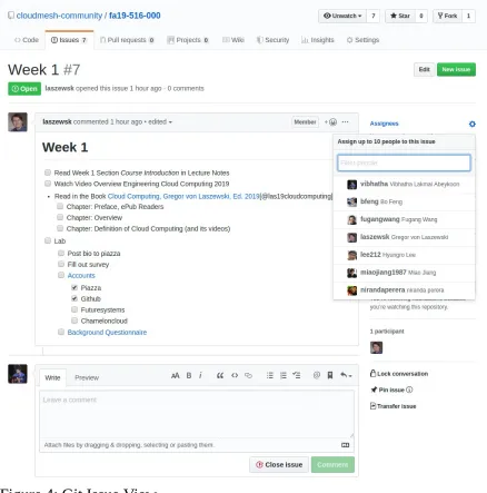
12.1.1.5 Step 5 (Optional)
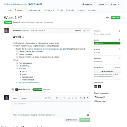
Figure 4: Git Issue View
12.1.1.6 Step 6 (Optional)