A Simulation Based Model for Determining Safety Inventory at a Fixed time Period System

Abstract: This paper develops a simulation model for determining safety inventory associated with a certain value of cycle service level in a fixed-time period system. The model takes into account actual amount of materials received from suppliers, and deviation from probability distribution of daily forecast demand. Constraints on order size are also embodied into the model. This model was constructed by using Visual Basic Application added in Microsoft Excel. After developing the model, hypotheses testing is employed to verify the model. This model allows identifying safety inventory under uncertain conditions which prohibits from the use of ordinary mathematical formula. The model was locally verified. Stochastic variables including customer demand and supplier’s lead time are assumed to be normally distributed. Independent demand items are considered and backorders are not allowed. Under specific conditions, such as distributions of demand and lead time are normally distributed, and fixed-time period system is being used. This model allows materials planner promptly identifies safety inventory associated with a certain level of cycle service level. Furthermore, planner can perceive the affects of changing input parameters on the amount of safety inventory required. There were very few researches focus on variations of demand and lead time at the same time. In reality, this case usually happens, thus the firms have been facing highly variations form both supplier and customers. Therefore, this paper intends to close this gap by simulating these factors and taken into account for determining safety inventory.

Keywords: independent demand, safety inventory, simulation, fixed-time period system,

I. INTRODUCTION

According to Chopra and Meindl (2016), inventory management is one of the three logistical drivers of supply chain management. Inventory appears in the supply chain in several forms, including raw materials, work-in-process (WIP), and finished product. The responsiveness and efficiency of a firm, or a supply chain as a whole, can be altered significantly by changes in inventory policies. Given a generic product, selecting the inventory policy for that product encompasses three major issues (Heizer and Render, 2008). Firstly, a method for auditing inventory must be established.

Revised Manuscript Received on October 05, 2019.

Le Tran Trung Kien is a Senior Production Engineer, Bosch Vietnam Co Ltd.

Azanizawati Ma’aram, Senior Lecturer, Faculty of Engineering, School of Mechanical Engineering, Universiti Teknologi Malaysia (UTM).

Syed Ahmad Helmi, Faculty Member, Faculty of Engineering, Universiti Teknologi Malaysia.

Aini Zuhra Abdul Kadir, Senior Lecturer, Faculty of Engineering, School of Mechanical Engineering, Universiti Teknologi Malaysia (UTM).

Auditing inventory may be carried out either on a continuous basis or on a periodic basis. Secondly, with respect to each method of auditing, the amount of product to be produced or to be purchased needs to be determined. Finally, a firm also has to make decision on which level of safety stock they should hold. This paper focuses on determining level of safety stock because it can be controlled flexibly by the firm, as long as they are able to fully guarantee other parties their service level.

Safety stock, also refers as buffer stock, is an amount of additional inventory carried to meet unexpected demand. A fixed-time period system, which is also known as periodic inventory system or periodic review system, refers to an inventory system in which amount of inventory in stock is identified after a fixed period of time, such as every week, or every month. Fixed-time period system is important because it can provide advantages of joint orders. Joint orders refer to a situation in which materials are transported in the same vehicle, purchased from the same supplier, or manufactured by the same machine. As a result, a significant reduction in ordering cost and shipping cost may be possible because items are processed under a single order and several items are ordered simultaneously (Tersine, 1994). The objective of this paper is to develop a simulation-based model calculating safety inventory under fixed-time period system when both daily demand and supplier’s lead time are normally distributed. The model consists of two main processes: simulation process and process of determining safety inventory.

II. LITERATURE REVIEW

Chopra and Meindl (2016) suggested a formula for identifying safety inventory under fixed-time period system when demand is normally distributed and lead time is constant. By using Microsoft Excel as a platform, Mielczarek and Zabawa (2002) employed Monte Carlo method to simulate a continuous inventory system (s, Q), where s is reorder point and Q is order quantity. The objective is to minimize total inventory cost, including holding cost, shortage cost, and ordering cost. Stochastic variables include daily demand and lead time. These variables are simulated by using Monte Carlo method. Data of these variables is collected from observations of past orders. Then, the historical frequencies will be converted into a probability distribution and cumulative distribution for simulation purpose. Other fixed parameters include beginning inventory, ordering cost, holding cost, and shortage cost.

The authors aim to find a combination of Q and s, which provides the lowest total inventory cost. In order to validate the model, they utilize ANOVA

to compare the outcomes of this

A Simulation-Based Model for Determining

Safety Inventory at a Fixed-time Period System

model with results that Heizer and Render (2001) obtained by using the same set of data.

A simulation model was built by Garcia et al. (2002) in order to test the validation of an analytical expression which Garcia and Machado (2001) developed to determine appropriate safety stock levels. The model simulates a periodic review inventory system with lot-for-lot replenishment principle, i.e., orders equal net requirements. The difference between quantity received and order placed is considered as random variable. This uncertainty exists because of defective items found in supplier’s shipment; fail in quality control, and difference between actual production output and desired rate may also occurred. In addition, uncertainties are also appeared in customer’s demand. Input parameters include forecasting of demand, probability distribution of deviation between demand and forecast, probability distribution of deviation between quantity ordered and quantity effectively received, cycle service level (CSL), and on-hand inventory at the first period. After that, the model simulates these two probability distributions, which are assumed to be normally distributed, to obtain actual demand and order quantity received. And then, safety stock and on-hand inventory at the end of each period are calculated. Output parameter is CSL, i.e., percentage of periods that on-hand inventory is larger than 0, obtained by simulation. Finally, the value of CSL provided by simulation is compared with expected value of CSL according to normal distribution, which is one of the inputs. The absolute deviation between them is expected to be as small as possible. If the deviation is small, it means that there is a good agreement between simulation model and theoretical expression. In other words, the authors expect that the simulated model converges to normal distribution. Based on absolute deviation obtained, the study shows that the analytical expression is adequate and valid to many practical cases. In this model, lead time is constant whereas forecasted demand and quantity of inventory received from supplier are stochastic. Verification is conducted at three level of cycle service level (CSL): 99.865% (3σ), 97.725% (2σ), and 84.135% (1σ).

III. SIMULATIONPROCESS

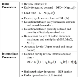
Table 3.1 shows two groups of parameters included in the model. These parameters will be described in detail.

A. Input Parameters

In periodic review policy, inventory levels are reviewed after a fixed period of time. This fixed period of time is called review interval (T), which is the time between successive orders. Daily forecasted demand is future demand projected for the coming periods on a daily basic. Forecasted demand of each day (DFDi) is a random variable and follows normal

distribution (µF,σ2F).

Lead time for replenishment (L) is the gap between when an order is placed and when it is received, and also follows

normal distribution (µL, ).

Desired cycle service level (CSL0) is expected likelihood that at least one stock-out will not happen within a replenishment cycle.

Table 1.1.Model Parameters Input

Parameters

 Review interval (T)

 Daily forecasted demand – DFD ~ N (µF, )  Lead time – L ~ N (µL, )

 Desired cycle service level – CSL (%)

 Deviation between daily forecasted demand and actual demand – r

 Deviation between quantity ordered and quantity effectively received – a

 Restrictions on size of order: minimum, maximum, and multiplier (MIN, MAX, MUL)

 Accuracy levels (Upper bound and lower bound)

Intermediate Parameters

 Demand during review interval and lead time -

 Estimated safety inventory – ESS (units)

 Order up-to-level – OUL (units)

Garcia et al. (2002) demonstrated deviation between forecasted demand and actual demand by using a random variable which is defined by:

Where

ri: the quantifier of deviation between forecasted and actual

demand.

DADi: daily actual demand on day i

DFDi: daily forecasted demand on day i

Due to quality issues and variability in production yield, quantity received at consignee’s dock is likely to be different from the amount which was ordered before. To quantify the deviation, Garcia et al. (2002) employed a random variable which is defined by:

Where:

ai: quantifier of deviation between quantity ordered and

quantity received

POi: planned order on day i

SRt: schedule receipt on day t, associated with planned order

on day i

This project acknowledges the contribution of Garcia and his followers, and assumes that these random variables ri and ai

are normally distributed, i.e. ri ~ N (µri,σri) and ai ~ N (µai,σai),

respectively.

There are three types of constraints on order size: maximum size (MAX), minimum size (MIN), and multiplier (MUL). These constraints are summarized

MIN ≤ Order Size ≤ MAX, and Order Size = MUL × Integer Number (3.3)

Accuracy levels, including Upper bound and Lower bound, are used to evaluate average of simulated cycle service level (CSL1). It is necessary for a quick evaluation. If CSL1

satisfies expression 3.22, the process of revising safety inventory is terminated and the current amount of safety inventory is considered as a solution.

CSL0 – Lower bound < CSL1 < CSL0 + Upper bound

(3.4)

B. Intermediate Parameters

Given the above inputs, another three intermediate parameters are determined. They include demand during lead time and review interval (DTL), estimated safety inventory (ESS), and order up-to-level (OUL).

According to Chopra and Meindl (2016), distribution of forecasted demand during review interval and lead time, when demand is normally distributed and lead time is stable, is as follows:

With:

And

Where:

DTL: demand during review interval and lead time T: review interval (days)

average demand during lead time

standard deviation of demand during lead time

average of daily forecasted demand

standard deviation of daily forecasted demand

: average lead time

Based on distribution of demand during review interval and

lead time, and given cycle service level, estimated safety

inventory (ESS) is calculated as follow:

Where:

ESS: estimated safety inventory

inverse of standard normal cumulative distribution

CSL0: desired cycle service level

(Chopra and Meindl, 2016) Order up-to-level (OUL) is calculated as follow:

OUL = ESS + µDTL (3.9)

Where:

µDTL: average demand during review interval and lead

time

ESS: estimated safety inventory

(Chopra and Meindl, 2016)

C. Process

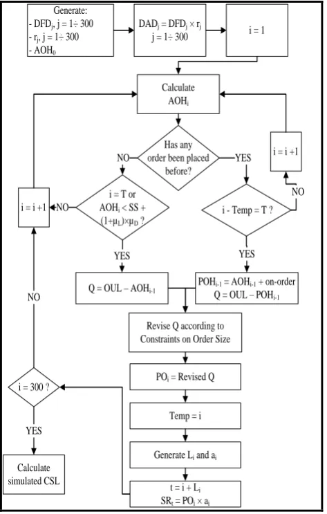
Figure 3.1 illustrates the mechanism of simulation model. This mechanism is described in the following paragraphs.

Actual On Hand Inventory (AOH) and Projected On Hand Inventory (POH)

Actual on hand inventory (AOH) is the actual inventory maintained at the end of each period. Actual on hand inventory at the end of day 0 (AOH0) is assumed as a random

variable which is evenly distributed from PSS to PSS + µF ×

T. This assumption bases on the fact that on hand inventory most likely falls into this range if unusual demand does not happen. So,

PSS ≤ AOH0 ≤ PSS + µF × T (3.10)

Where:

PSS: proposed safety inventory (units)

µF: average of daily forecasted demand

T: review interval

Because backorder is not allowed; therefore, actual on hand inventory at the end of day i (AOHi) is calculated as follow:

AOHi = AOHi-1 + SRi – DADi if AOHi-1 > 0 (3.11)

AOHi = SRi – DADi

if AOHi-1 < 0 (3.12)

Where:

AOHi-1: actual on hand inventory on day i-1

SRi: schedule receipt on day i

Generate: - DFDj, j = 1÷ 300

- rj, j = 1÷ 300

- AOH0

Calculate AOHi

t = i + Li

SRt = POi × ai

Calculate simulated CSL

Generate Li and ai

i = 1

Has any order been placed

before? NO

POHi-1 = AOHi-1 + on-order

Q = OUL – POHi-1

i = T or AOHi < SS +

(1+µL)×µD ?

NO i = i +1

YES

Q = OUL – AOHi-1

i = 300 ? NO

YES

Temp = i

i - Temp = T ? YES i = i +1

NO

YES DADj = DFDj × rj

j = 1÷ 300

Revise Q according to Constraints on Order Size

POi = Revised Q

Figure 3.1: Simulation Process

Projected on hand inventory (POH) is the projected inventory position which takes into account the amount of actual on hand inventory (AOH) and the amount of purchased orders (PO) which have not been received yet. Projected on hand inventory at the end of day i (POHi) is calculated as follows:

POHi = POHi-1 + POi – DADi , if AOHi > 0 (3.13)

POHi = POHi-1 + POi – (DADi + AOHi)

if AOHi < 0 (3.14)

Where:

POi: planned order at the beginning of day i

DADi: daily actual demand on day i

Planned Order (POi) and Schedule Receipt (SRi)

At the end of every cycle (review interval - T days), it requires that the systems reviews projected on hand inventory (POH). If POH is lower than order up-to-level (OUL), an order needs to be placed on the beginning of the next day, which is the first day of the next review cycle. This order is called planned order (PO). Planned order at the beginning of day i (POi) is

identified as follow:

POi = OUL – POHi-1 (3.15)

Where:

OUL: order up-to-level

POHi: projected on hand inventory at the end of day i

Planned order at the beginning of day i (POi) is revised

according to constraint on order size. After that, a random

variable, which is called lead time (Li), associated with this

POi is generated.

The actual arrival of POi after Li (lead time) days is called

Schedule Receipt at the beginning of day (i + L), which is denoted as SRt, t = i + Li. So, schedule receipt at the

beginning of day t is determined as follow:

SRt = POi × ai (3.16)

Where:

POi: planned order on the beginning of day i

ai: order quantifier associated with POi

t = Li + i

Li: lead time associated with POi

D. Process of Determining Safety Inventory

Figure 4.1 presents processing of determining safety inventory. This process is going to be described in detailed on the follow sections.

Revising proposed safety inventory

If a proposed safety inventory (PSS) does not satisfy accuracy level or is rejected after conducting verification, it is revised by adding or subtracting a certain amount of inventory. After revising, a new PSS is created and inserted in final model to determine average of simulated cycle service level (CSL1).

The amount of inventory added to or subtracted from the PSS depends on magnitude of error and CSL1 itself. The error is

the difference between CSL1 and desired cycle service level

(CSL0), defined as follow:

Error = CSL0 – CSL1 (4.1)

Equation 3.7 (to calculate Safety

Inventory)

Input Data Estimated

Safety Inventory

Simulation Process

Revising Safety Inventory

Simulated Cycle Service Level (CSL1)

Satisfy accuracy

level ?

Accept Revised Safety Inventory

Reject ? Verification NO

YES

YES

NO Legends:

Process

Data

Proposed Safety Inventory (PSS)

Figure 4.1: Process of determining safety inventory

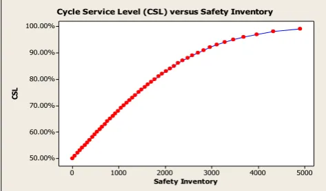
Value of CSL1 also affects the

that, by adding a fixed amount of inventory to safety inventory, marginal increase in cycle service level reduces as the value of cycle service level increase. Diminishing return principle is applied here. This statement is illustrated by Figure 4.2.

5000 4000

3000 2000

1000 0

100.00%

90.00%

80.00%

70.00%

60.00%

50.00%

Safety Inventory

CS

L

Cycle Service Level (CSL) versus Safety Inventory

Figure 4.2: Cycle Service Level versus Safety Inventory Proposed safety inventory (PSS) is calculated by the following formula:

PSSt = PSSt-1 – Error × Dij (4.2)

Where:

PSSt: Proposed Safety Inventory at loop t

Error: difference between CSL1 and CSL0

Dij: Estimated average amount of change in PSS in order to

increase or decrease 1% in CSL, Dij is defined in table 3.9

Table 3.1: Average Inventory Needed to Change 1% in Cycle Service Level

Cycle service

level (CSL)

Estimated safety inventory

(ESS)

Estimated inventory needed to change 1% in

CSL (Dij)

80% ESS1

85% ESS2 D12 = (ESS2 – ESS1) / 5%

90% ESS3 D23 = (ESS3 – ESS2) / 5%

95% ESS4 D34 = (ESS4 – ESS3) / 5%

99% ESS5 D45 = (ESS5 – ESS4) / 4%

For example, if CSL1 is equal to or lower than 85%, D12 is used to calculate PSS. If CSL1 is greater than 85%, and equal to or lower than 90%, D23 is used.

E. Model Verification

A model, which considers fluctuations in customer’s demand and supplier’s lead time, deviation between planned order and schedule receipt, and constraints on order size, has not been found from literature review. Therefore, the model is run under special input conditions which make it identical to a theoretical model discussed by Chopra and Meindl (2016). This theoretical model assumes the followings. Firstly, distributions of daily forecasted demand and daily actual demand are identical. Secondly, there is no difference between scheduled receipt and planned order. Thirdly, there is no constraint on order size. Finally, lead time is constant. By doing, the result obtained from the simulation model can compare with the result calculated by the theoretical model. Special conditions are described in table 4.2.

Table 4.2: Special Conditions of Inputs

No. Inputs Special Conditions

1 Demand quantifier - ri

2 Order quantifier - ai

3 MIN, MAX, MUL MIN = 0, MAX ≈ ∞, MUL =

1

4 Lead time - L σL

Other numerical inputs are shown in table 4.3.

Table 4.3: Other Numerical Inputs

No. Inputs Numerical value

1 Daily forecasted demand (DFD)

N (2500, 502)

2 Lead time (L) 2 days

3 Review interval (T) 4 days

4 Desired cycle service level (CSL0)

90%

5 Accuracy levels Lower bound = 0.1%

Upper bound = 0.1% The model was run 30 replications. Proposed safety inventory (PSS) at each replication was recorded and shown in table 4.4.

Table 4.4: Running Experiment for Verification Replicatio

n

PSS Replicatio n

PSS Replicatio n

PSS

1 1548 11 1548 21 1611

2 1607 12 1611 22 1498

3 1566 13 1592 23 1607

4 1592 14 1465 24 1551

5 1544 15 1566 25 1488

6 1572 16 1622 26 1583

7 1613 17 1557 27 1563

8 1551 18 1560 28 1598

9 1546 19 1531 29 1585

10 1569 20 1526 30 1547

Average ₁₅₆₄

Std. Dev. s = 38

According to Chopra and Meindl (2016), regarding to this particular case, safety inventory required to satisfy CSL = 90% is 1570 (units). Hypothesis testing was conducted to compare mean of proposed safety inventory and 1570 (units).

Hypotheses (α = 0.05): H0 : μPPS = 1570

H1 : μPPS ≠ 1570

Sample size, n = 30

Test statistics, = − 0.865

t-value, t0.05/2, 29 = 2.054

Because t-value is larger than absolute value of test statistics, null hypothesis cannot be rejected. In other words, mean of proposed safety inventory is not

1570 units. Therefore, it can be concluded that there is a strong agreement between the proposed simulation model and the theoretical model. As a result, the proposed model is locally verified.

IV. CONCLUSION

A simulation-based model for determining safety inventory under fixed-time period system was fully developed and then verified using specified inputs. The model takes into account the fluctuations in the amount of materials received from suppliers, lead time and customer demand. Constraints on order size are also embodied into the model. The proposed model allows user to quickly identify safety inventory which can absorb the above fluctuations.

ACKNOWLEDGMENT

Our special thanks go to the Universiti Teknologi Malaysia (UTM) for its partly financial support (Grant awarded: Transdisciplinary Research Grant (TDR) with registration number Q.J130000.3551.07G15).

REFERENCES

1. Chopra, S. and Meindl, P. (2016). Supply Chain Management: Strategy, Planning, and Operation. (6th ed.). Upper Saddle River, N. J.: Prentice Hall.

2. Garcia, E. S., Silva, C. F. and Saliby, E. (2002). A Simulation Model to Validate and Evaluate the Adequacy of an Analytical Expression for Proper Safety Stock Sizing. Proceedings of the 2002 Winter Simulation Conference. 8-1 Dec 2002, San Diego, CA, USA, pp. 1282-1288.

3. Heizer, J., and Render, B. (2008). Operations Management. (9th _ed.). Prentice Hall International, Inc.

4. Montgomery, D. C. (2009). Statistical Quality Control: A Modern Introduction. (6th ed.). John Wiley & Sons, Inc.

5. Tersine, R. J. (1994). Principles of Inventory and Materials Management. (4th _{ed.). Prentice Hall International, Inc.}

6. Zabawa, J. and Mielczarek, B. (2007). Tools of Monte Carlo Simulation in Inventory Management Problems, Proceedings 21st European Conference on Modelling and Simulation, Ivan Zelinka, Zuzana Oplatková, Alessandra Orsoni, pp. 1-6.

AUTHORSPROFILE

Le Tran Trung Kien is a Senior Production Engineer at Bosch Vietnam Co Ltd. He works in several companies including Schneider Electric (Clipsal Vietnam) and Jabil Vietnam as a process engineer and industrial engineer respectively. He obtained his Bachelor of Industrial Systems Engineering from Ho Chi Minh University of Technology, Vietnam. He did Diploma in Logistics in Singapore Institute of Materials Management (SIMM). Then he pursued his Master of Science (Industrial Engineering) in Universiti Teknologi Malaysia and received the Best Student Award. He certified Basic MOST Certificate (Maynard Sequence Technique) from Accenture Workforce Optimization Academy. His research interests are process optimization, capacity planning, simulation of industrial systems and solving industrial problems.

Azanizawati Ma’aram is a senior lecturer at the School of Mechanical Engineering, Faculty of Engineering, Universiti Teknologi Malaysia (UTM). She obtained her Bachelor of Engineering (Mechanical-Industrial) and Master of Engineering (Advanced Manufacturing Technology) from Universiti Teknologi Malaysia, Malaysia. She pursued her Doctorate of Philosophy (Ph.D) (Management) at the University of Liverpool, United Kingdom. She has held several positions including Head of Industrial Panel, Postgraduate Coordinator for Master of Science (Industrial Engineering), and Laboratory Coordinator for Industrial Engineering. She is a member of the International Association of Engineers (IAENG), the Board of Engineers (BEM) Malaysia and the Malaysia Board of Technologists (MBOT). She has taught courses in industrial engineering, supply chain management

(undergraduate and postgraduate levels), engineering management and safety, work design, ergonomics and research methodology. Her research interests include supply chain management, performance measurement, lean manufacturing, sustainability, ergonomics and safety. She is currently active as a Project Leader and a Project Member on numerous research projects and has secured several grants funded by the university and Ministry of Education (MoE) that involve hospitals and industrial collaborators.

Syed Ahmad Helmi is a faculty member at the Faculty of Engineering, Universiti Teknologi Malaysia. He received his Bachelor of Science in Mechanical Engineering, Master of Engineering in Advanced Manufacturing, and PhD in Engineering Education. He is currently a fellow at the Centre for Engineering Education, and head of the university Research Group in Engineering Education (RGEE). Prior to joining UTM, he worked as a maintenance engineer at INTEL, Malaysia, as research officer at the Standard and Industrial Research Institute of Malaysia (SIRIM), and as mechanical and industrial engineer at Sime-Darby, Malaysia. His research focuses on Mechanical Engineering, Industrial Engineering and Engineering Education. His recent work includes academic change management, complex engineering problems, manufacturing systems and optimization, supply chain, and systems dynamic modelling. Over the years, he has conducted several workshops on Outcomes-Based Education (OBE) particularly in Student Centred Learning (SCL) throughout Malaysian Higher Institutions, and International Institutions such as in Indonesia, Korea, India, China, Turkey, Morocco, South Africa, Pakistan, and Afghanistan. Throughout his career he received several awards such as excellent service awards, best paper awards, and gold medals in innovative practices in higher education. He has published several books and more than 80 papers in journals and conference proceedings.

Nor Hasrul Akhmal Ngadiman received his Bachelor of Engineering in Mechanical Engineering (Industry) degree from Universiti Teknologi Malaysia (UTM) in 2012. Based on his excellent achievement in academic and extra-curricular activities, he was offered the opportunity to pursue his Doctor of Philosophy (PhD) degree directly after his first degree via UTM’s Fast Track Programme. He embraced the challenge, and with diligence and perseverance he obtained his PhD in Mechanical Engineering from UTM in 2016. He is currently Senior Lecturer in the Department of Materials, Manufacturing and Industrial Engineering, School of Mechanical Engineering, Faculty of Engineering (FE), UTM, Johor Bahru, Johor, Malaysia. Dr. Hasrul is involved (both as Project Leader and Project Member) in numerous research projects funded by the Ministry of Education and various industries as well as by the UTM. His papers have been published in both international and national journals. In addition to this, he has presented papers at international and national conferences and seminars and obtained over 94 citations and H- index 6. Dr. Hasrul is engaged with several consultancy projects involving local companies and organizations and has conducted training on diverse courses organized by the university.