Abstract: Data mining is a key research field in the computer science research arena. Feature selection is performed once the dataset got cleansed. Optimization algorithms are considered to be helpful for the feature selection task. Also the obtained suitable features will contribute considerably for the classifier. Machine learning classifiers are comparatively performing better than that of traditional data mining classification algorithms. In this part of research work an adaptive particle swarm optimization algorithm is employed in order to perform feature selection task. Extreme learning machine classifier is added with credential weights. Twenty datasets are taken for performance analysis. From the obtained results it is evident that Adaptive Particle Swarm Optimization based Credentialed Extreme Learning Machine Classifier (APSO-CELMC) performs better in terms of predictive accuracy and time taken for classification.
Index Terms: Machine learning, feed forward neural network, extreme learning machine, optimization, particle swarm, swarm intelligence, high dimensional datasets..
I. INTRODUCTION
Data mining is one of the active research areas in the field of computer science as well as information technology. During the past two decades there is a knowledge data discovery progression assists the data mining to pull out hidden information from the dataset, there is a mammoth amount of machine learning algorithms to be incorporated for performing data mining tasks. For the most part supervised machine learning algorithms augment leading implication in the research field of data mining. Machine learning shortly termed as ML is a type of artificial intelligence (AI) that make available computers with the capability to be trained without being transparently programmed. ML learning focuses on the spreading out of computer programs that can adapt as well as adjust at the point of time uncovered to new-fangled data. ML algorithms are broadly classified into three categories namely supervised
Revised Manuscript Received on July 08, 2019.
M.Praveena, MCA,M.Phil, Asst.Professor, Department of Computer Science, Dr.SNS Rajalakshmi College of Arts and Science, Coimbatore-49. Tamilnadu, India.
Dr.V. JAIGANESH, MCA, M.Phil, MBA, Ph.D., Professor, Department of PG and Research in Computer Science, Dr. N.G.P. Arts and Science College, Coimbatore - 641 048. Tamilnadu, India.
learning, unsupervised learning and reinforcement learning and is shown in Fig.1. The succession of machine learning is corresponding to that of data mining. Both data mining and machine learning examine as well as search from end to end data to seem for patterns. Conversely, in penchant to extracting data for human knowledge as is the case in data mining applications; machine learning employs data to recognize patterns in data and tweak program actions henceforth.
Fig.1. Machine Learning and its Types
Supervised machine learning is the task of inference a meaning from labeled training data that consists of a collection of training examples. As far as supervised learning is concerned, each instance is a brace encloses an input object (which is usually a vector quantity) and a vital output value (may also be referred as supervisory signal). Initially, the supervised learning algorithm does the analysis task from the training data and builds a dependent function, for mapping new examples. An optimal setting possibly makes possible the algorithm to precisely determine the class labels for covered instances and the same requires the supervised learning algorithm to make simpler from the training data to covered situations in a "balanced" manner. The supervised algorithms / methods are probably used in a variety of application areas that include marketing, finance, manufacturing, testing, stock market prediction, and so on. This research work aims in proposing a Adaptive Particle Swarm Optimization based Credentialed Extreme Learning Machine Classifier (APSO-CELMC) for High Dimensional Datasets. The aim of ISVMC is to improve the prediction accuracy and also to decrease the time taken for classification. The paper is organized as follows. This section introduces the work. Section 2
gives some of the related works. Section 3 portrays the proposed work. Section 4 presents results
Adaptive Particle Swarm Optimization based
Credentialed Extreme Learning Machine
Classifier (APSO-CELMC) for High
Dimensional Datasets
and discussions. Section gives the concluding remarks.
II. RELATED WORKS
Feature selection is the method of selecting a set of representative features / dimensions [1] which have high correlation with the output variables (forecasting variables). Researchers applied a variety of feature selection methods. I. Koprinska et al. [1] evaluated the performance of four feature selection methods (Autocorrelation, Mutual Information, RRelief (RF), Correlation-Based Selection (CFS). The conclusion was that the better prediction models were RF+NN and AC+NN for the data experiments [1]. The results from the research of R. Mashud et al. [2] showed that CFS [3] and Mutual Information were able to identify a small set of informative lag variables, that when used with LUBEX [4] resulted in good quality PIs (prediction interval) for interval forecasting of electricity demand time series data. M. M. Mafarja et al. [5] used binary DA to overcome feature selection, and they obtained a good experimental result when the input feature is large. M. Mafarja et al. [6] proposed evolutionary population dynamics and grasshopper optimization approaches for feature selection problems, which is good at handling a large number of input features and is limited when the number of features is small. Good features often can accelerate the process of establishing model and helping model to improve the forecasting performance.
It is noteworthy that existing structural classifiers do not balance structural information’s relationships both intra-class and inter-class. Combining the structural information with nonparallel support vector machine (NPSVM), D. Chen et al. 2016 [10], designed a new structural nonparallel support vector machine (called SNPSVM). Each model of SNPSVM considers not only the compactness in both classes by the structural information but also the separability between classes, thus it can fully exploit prior knowledge to directly improve the algorithms generalization capacity. Moreover, the authors applied the improved alternating direction method of multipliers (ADMM) to SNPSVM. Both their model itself and the solving algorithm can guarantee that it possibly would deal with large-scale classification problems with a huge number of instances as well as features. Experimental results show that SNPSVM is superior to the other current algorithms based on structural information of data in both computation time and classification accuracy.
Peng et al., 2016 [11] formulated a linear kernel support vector machine (SVM) as a regularized least-squares (RLS) problem. By defining a set of indicator variables of the errors, the solution to the RLS problem is represented as an equation that relates the error vector to the indicator variables. Through partitioning the training set, the SVM weights and bias are expressed analytically using the support vectors. The authors also demonstrated how their approach naturally extends to sums with nonlinear kernels whilst avoiding the need to make use of Lagrange multipliers and duality theory. A fast iterative solution algorithm based on Cholesky
decomposition with permutation of the support vectors is suggested as a solution method. The properties of their SVM formulation were analyzed and compared with standard SVMs using a simple example that can be illustrated graphically. The correctness and behavior of their proposed work has been demonstrated using a set of public benchmarking problems for both linear and nonlinear SVMs. In recent years an approach for training single-hidden layer feed forward neural networks called Extreme Learning Machines (ELM) have been proposed [12], [13] and extensively investigated. Several topics around ELMs are subject to discussion as they are considered similar to, or special cases of, radial basis 110 function (RBF) networks, random vector functional-link (RVFL), least squares support vector machines (LS-SVM), or reduced SVM [14], [15], [16], but they are outside of the scope of this research work. Among the attractive features of ELM networks are the use of a single hidden layer, high training speed, good generalization/accuracy. It has been found that in certain applications characterized by noisy data, like image recognition, ELM’s do not exhibit good performance. However, new ELM algorithms overcome the problem, providing excellent generalization and classification performance [17], [18].
III. PROPOSED WORK
In this research work PSO is used for feature selection. The fitness is measured using the input obtained from the output of ELM. After that classification is performed by credentialed ELM classifier.
3.1. Particle Swarm Optimization for Feature Selection
PSO is a meta-heuristic search technique that simulates the flock of bird’s movements to find the food. Each particle in the swarm represents a candidate solution that flies through the multidimensional search space. A particle uses the best position explored by itself and that of its neighbors to move towards an optimum solution. The performance of each particle (i.e. the “closeness” of a particle to the global minimum) is measured according to a predefined fitness function.
Suppose that the search space is D-dimensional and there are m particles in the swarm. Each particle is located at
position
X
i
x
i1,
x
i2,
.
.
.
,
x
iD
withvelocity
V
i
v
i1,
v
i2,
.
.
.
,
v
iD
, wherei
1
,
2
,
.
.
.
,
m
. In the PSO algorithm, each particle moves towards its own bestposition
pbest
denoted as
i ii iD
i
pbest
pbest
pbest
Pbest
1,
2,
.
.
.
,
and the best
position of the whole swarm
gbest
denotedas
Gbest
gbest
1,
gbest
2,
.
.
.
gbest
D
. And eachparticle changes its position according to its velocity, which is randomly generated towards
For each particle,
i
and dimensions
, the new velocityis
v
and position
x
iscan be calculated by the equations (1)and (2):
1 1
2 2 1 1 1
1
1
t
s t s t
is t is t
is t
is wv cb pbest x cb gbest x
v … (1)
t is t is t
is
x
v
x
1
… (2)
Where
t
is the iteration number. The inertial weightw
is used to control the velocity and balance of the exploration and exploitation abilities of algorithm. A large value ofw
keeps particles at high velocity and prevents them frombecoming trapped in the local optima. A small value of
w
maintains particles at low velocity and encourages them toexploit the same search area. The constants
c
1 andc
2arecalled acceleration coefficients that determine whether
particles prefer to move closer to the
pbest
orgbest
positions. Theb
1 andb
2 are independent randomnumbers uniformly distributed between 0 and 1. The termination criterion of the PSO algorithm includes the maximum number of generations, the designated value
of
pbest
, or no further improvement inpbest
. A PSO based feature selection is presented in this work that determines the importance of features by ranking them and uses the information to improve the search ability of algorithm.Measuring the fitness
It is well known that feature selection is the choice of a small number of relevant features to obtain similar or even better classification performance than that of the use of all features. Thus, in this phase of research two main conflicting objectives are taken into account that represents the classification performance and the number of features; both objectives should be minimized. The first objective, classification performance, is error rate, which is calculated via equation (3) for
i
-th particle:
FP FN
FP FN TP TN
rateError_ i / … (3)
TN
FP
TP
,
,
andFN
refer to true positives, falsepositives, true negatives, and false negatives of CELM classifier, respectively.
The second conflicting objective considers the number of selected features. Small number of features reduces the computational cost yet increases the error rate. As normalized values of the objectives provide a uniform search of the problem space, second objective should be calculated according to the equation (4) for i-th particle:
D
j j i i i
i f D f Z t
rate Feature
1 , / _
… (4)
Where, D is the total number of features. In this fashion, both objectives are normalized in [0,1]. External archive is used to store the non‐dominated solutions found during the search. After calculating the fitness function, the non-dominated solutions are extracted, and the archive set is updated.
Feature Ranking and Selection
The selected features by the archive members are more important than the other features. Therefore, the archive can rank the features. They are ranked based on the equation (5).
Ak
k
k
t
Z
t
A
Z
FR
1
,
… (5)
Set
A
represents the archive andZ
k
t
is a decodedmember of archive. In this way,
FR
is a vector withD
dimensions as
r
r
r
D
FR
1,
2,
.
.
.
,
that,r
j,
j
1
,
2
,
.
.
.
,
D
, determines
the rank of
j
-th feature. The minimum value ofr
j is zero when thej
-th feature is not selected by any member ofarchive. The maximum value of
r
j is equal to the length of the archive when thej
-th feature is selected by all members of archive.3.2. Extreme Learning Machine
After the feature selection is performed, ELM is used for performing classification task. Given a set of N training
instances
(
x
i,
t
i)
and 2L hidden neurons altogether (that is, each of the two covered layer has L covered neurons) with the initiation work g (x). At first arbitrarily introduce the association weight matrix between the info layer and the first covered layer W and the inclination matrix of the first hidden layer B, and afterward figure the weight matrix β between the second hidden layer and the outcome layer.1
1
)
(
W
H
B
H
g
H
... (8)where
W
Hindicates the weight matrix between the firstcovered layer and the second hidden layer. It is assumed that the first and second hidden layers have a similar number of
neurons, and subsequently
W
H is a square matrix. Thedocumentation H indicates the outcome between the first hidden layer as for all N preparing tests. The matrices
1
1
and
H
B
individually speak to the inclination and thenormal outcome of the second covered layer.
The normal outcome of the second covered layer can be ascertained as
T
1
H
... (9)
where β† is the MP widespread contrary of the matrix β. The manipulative means of β† is the alike as before discussed
for H†, namely
†
(
T
)
1
Tif
T
isnonsingular, or alternatively
T T
if
† T 1)
(
is nonsingular. Consequently it is defined the augmented
matrix
W
HE
[
B
1W
H]
, and calculate it as† 1 1
)
(
EHE
g
H
H
W
... (10)
where
†
E
H
is theT
E
H
H
[
1
]
, 1 denotes a one-column vector of size Nwhose components are the scalar unit 1, where the notation
g(x) denotes the contrary of the calculation of
†
H
proceeds in the fashion described some time recently. The investigations directed to test the execution of the ELM calculation. In order to perform the classification task extensively used logistic sigmoid function g (x) =
)
1
/(
1
e
xis used. The real outcome of the second covered layer is calculated as
)
(
2
g
W
HEH
EH
... (11)and finally, the mass matrix
newflanked by the secondcovered layer and the real layer is calculated as
T
H
2†new
... (12)
where
† 2
H
is the MP widespread contrary ofH
2, gottenutilizing the approach talked about some time recently. The ELM outcome in the wake of preparing can be communicated as
f(x) =
H
2
new... (13)3.3. Credentialed – ELM Classifier (CELMC)
CELM aims to perform the classification task among heterogeneous data where class imbalance problem is quite challenging. In CELM each training instance is assigned an additional credential. The credential associated with the minority class instances is comparatively higher than that of the majority class instances. This strengthens the impact of the minority class instances relative to the majority class instances. The two credential schemes were experimentally employed to calculate the credential matrix CL, which are automatically generated using the class distribution by using the following equations:
k ii
q
CL
1
… (14)
Where qk is denotes the total number of instances
belonging to the class k.
The next credential mechanism:
)
(
1
)
(
611
.
0
avg k
k
avg k k
ii
q
q
if
q
q
q
if
q
CL
… (15)
Here, qavg denotes the average number of instances per
class. Credential, CLii is assigned to the ith instances. The
mathematical model of CELM is given below
2 1 2
2 1 2 1
: i
N i CLii
C
Minimize
… (16) Algorithm 1. CELM Algorithm Input: N training instances X =
T N
x
x
x
,
,
...
,
]
[
1 2 , T =T N
t
t
t
,
,
...
,
]
[
1 2and 2L hidden neurons in total with activation function g (x)
1: Haphazardly create the association weight matrix between the information layer and the first covered layer W and the inclination matrix of the first hidden layer B and for
straightforwardness,
W
IEis defined as[ B W] and likewise,E
X
is defined as[
1
X
]
T .2: Calculate
H
g
(
W
IEX
E)
:3: Acquire weight matrix between the second covered layer and the outcome layer β =
H
†T
4: Compute the normal outcome of the second hidden layer
†
1
=
T
H
5: Decide the parameters of the second covered layer (association weight matrix between the first and second hidden layer and the predisposition of the second covered
layer)
† E 1 1
)
(
H
H
g
W
HE
6: Acquire the real outcome of the second hidden layer
)
(
2
g
W
HEH
EH
7: Recalculate the weight matrix between the second
covered layer and the outcome layer new
H
T
† 2
The final output of CELM is
new
H
g
W
X
B
B
W
x
f
(
)
{[
(
)
1]}
.
IV. RESULTS AND DISCUSSIONS
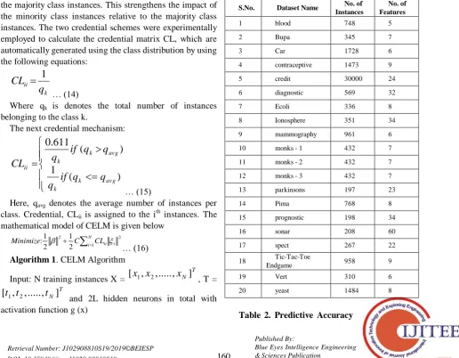
Table 1. Dataset Name, No. of Instances and No. of Features
S.No. Dataset Name No. of Instances
No. of Features
1 blood 748 5
2 Bupa 345 7
3 Car 1728 6
4 contraceptive 1473 9
5 credit 30000 24
6 diagnostic 569 32
7 Ecoli 336 8
8 Ionosphere 351 34
9 mammography 961 6
10 monks - 1 432 7
11 monks - 2 432 7
12 monks - 3 432 7
13 parkinsons 197 23
14 Pima 768 8
15 prognostic 198 34
16 sonar 208 60
17 spect 267 22
18 Tic-Tac-Toe
Endgame 958 9
19 Vert 310 6
20 yeast 1484 8
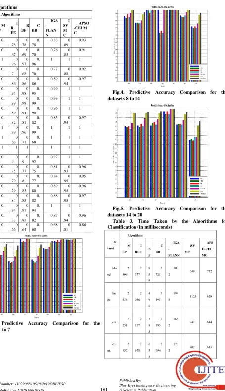
[image:4.595.46.563.429.831.2]of the Algorithms Dat aset Algorithms M LP T R EE R BF C BB IGA - FLAN N I SV M C APSO -CELM C blo od 0. 8 0 .78 0 .78 0. 78
0.83 0
.89 0.93 bup a 0. 7 0 .67 0 .69 0. 70
0.76 0
.85
0.91
car 1 0
.96 0 .97
0. 96
1 1 1
con t. 0. 72 0 .7 0 .68 0. 70
0.77 0
.88 0.92 cre dit 0. 87 0 .86 0 .86 0. 86
0.89 0
.94 0.97 dia g. 0. 97 0 .95 0 .98 0. 95
0.99 1 1
eco li 0. 99 0 .99 0 .98 0. 99
0.99 1 1
ion o. 0. 91 0 .89 0 .94 0. 90
0.96 1 1
ma mm. 0. 82 0 .82 0 .81 0. 82
0.85 0
.94
0.97
mk s-1
1 0
.99 0 .96
0. 99
1 1 1
mk s-2
1 0
.68 0 .71
0. 68
1 1 1
mk s-3
1 1 1 1 1 1 1
par k 0. 92 0 .9 0 .9 0. 92
0.97 1 1
pim a 0. 77 0 .75 0 .77 0. 75
0.81 0
.93 0.96 pro g. 0. 8 0 .79 0 .8 0. 77
0.84 0
.95 0.95 son ar 0. 81 0 .79 0 .83 0. 80
0.89 0
.95 0.96 spe ct 0. 81 0 .84 0 .85 0. 82
0.88 0
.95
0.97
tic 0.
97 0 .94 0 .97 0. 94
1 1 1
vert 0. 82 0 .83 0 .83 0. 82
0.87 0
.94 0.96 yea st 0. 65 0 .66 0 .64 0. 68
0.68 0
.81
0.86
Fig.3. Predictive Accuracy Comparison for the datasets 1 to 7
Fig.4. Predictive Accuracy Comparison for the datasets 8 to 14
Fig.5. Predictive Accuracy Comparison for the datasets 14 to 20
Table 3. Time Taken by the Algorithms for Classification (in milliseconds)
Da taset Algorithms M LP T REE R B F C BB IGA - FLANN ISV MC APS O-CEL MC blo od 2 396 2 377 2 8 3 9 2 721 103
2 649 772
bu pa 2 436 2 056 2 4 9 6 3 193 194
8 1123 929
car 2 251 2 157 2 3 8 5 2 795 168 2
947 644
co nt. 2 157 2 978 2 6 3 5 2 696 173 2
[image:5.595.87.543.42.832.2] [image:5.595.43.278.51.719.2] [image:5.595.309.545.54.533.2]cre dit
1 9377
1 9563
1 9 6 7 4
1 9701
157 82
8099 6580
dia g.
7 361
7 233
7 6 7 6
7 790
398 2
2184 1608
eco li
2 268
2 367
2 6 6 5
2 686
184 6
799 676
ion o.
7 588
7 558
7 5 6 9
7 663
390 1
2001 1584
ma mm.
2 875
2 210
2 6 1 2
2 672
173 8
864 830
mk s-1
2 039
2 185
2 0 7 6
2 662
193 6
895 692
mk s-2
2 329
2 940
2 1 2 0
2 757
172 6
826 748
mk s-3
2 024
2 062
2 4 9 7
2 756
163 9
904 705
par k
4 047
4 526
4 8 7 9
4 731
239 3
1275 906
pi ma
2 052
2 813
2 9 9 2
2 797
139 2
780 535
pro g.
2 686
2 208
2 6 4 4
2 656
188 8
947 674
son ar
8 686
8 297
8 7 8 8
8 738
518 9
2548 1723
spe ct
5 348
5 655
5 4 5 5
5 804
229
1 1277 1066
tic 2 250
2 574
2 7 4 5
2 807
174
9 985 534
ver t
2 869
2 054
2 6 4 5
2 618
163
8 849 671
yea st
2 088
2 971
2 2 2 2
2 655
184 3
909 576
Fig.6. Time Taken for Classification by the Algorithms
Comparison for the
datasets 1 to 7
Fig.7. Time Taken for Classification by the Algorithms
Comparison for the
Fig.8. Time Taken for Classification by the Algorithms
Comparison for the
datasets 15 to 20
20 datasets are taken from the UCI machine learning repository namely blood, bupa, car, contraceptive, credit, diagnostic, ecoli, Ionosphere, mammography, monks – 1, monks – 2, monks – 3, parkinsons, pima, prognostic, sonar, spect, Tic-Tac-Toe Endgame, vert and yeast. The dataset details such as name of the dataset, number of instances and number of features are portrayed in the Table 1. The implementations are done using MATLAB tool. The system configuration is Core I3 processor with 8 GB RAM and 1 TB hard disk that runs on Microsoft Windows 8 operating system. Performance metrics such as predictive accuracy and time taken for classification are obtained. For better visual depiction at first 7 datasets are involved in the simulation followed up with next 7 datasets and finally with 6 datasets. It is evident from the results that the proposed APSO-CELMC outperforms all the other algorithms in terms of prediction accuracy. Next, we compared the performance of the proposed APSO-CELMC in terms of time taken for classification. From that results too, it is obvious that the proposed APSO-CELMC consumes less time than that of all the algorithms. The proposed APSO-CELMC algorithm is also compared with our previous works named IGA – FLANN [19] and ISVMC [20]. It is significant that APSO-CELMC performs better than that of IGA-FLANN and ISVMC in terms of predictive accuracy and elapsed time for classification.
V. CONCLUSION
This part of research work aim in two major data mining tasks namely feature selection and classification. An adaptive particle swarm optimization is used for performing feature selection and credentialed extreme learning machine is employed for classification. Twenty datasets are chosen for evaluating the efficiency of the classifier using the performance metrics predictive accuracy and time taken for classification. The obtained datasets are high dimensional in nature. Hence the fundamental component of feature selection by using particle swarm optimization algorithm
obtains fitness from extreme learning machine. The results are better in terms of the chosen performance metrics.
REFERENCES
1. I. Koprinska, M. Rana, V.G. Agelidis, et al., Correlation and instance based feature selection for electricity load forecasting, Knowl. Based Syst. (2015) 29–40.
2. M. Rana, I. Koprinska, A. Khosravi, Feature selection for interval forecasting of electricity demand time series data, in: Artificial Neural Networks, Springer Series in Bio-/Neuroinformatics, 2015, pp. 445–462. 3. M A. Hall, Correlation-based feature selection for discrete and numeric class machine learning, in: International Conference on Machine Learning, 2000, pp. 359-366.
4. A. Khosravi, S. Nahavandi, D.C. Creighton, et al., Lower upper bound estimation method for construction of neural network-based prediction intervals, IEEE Trans. Neural Netw. 22 (3) (2011) 337–346.
5. M.M. Mafarja, D. Eleyan, I. Jaber, et al., Binary dragonfly algorithm for feature selection, in: International Conference on New Trends in Computing Sciences, IEEE Computer Society, 2017, pp. 12–17. 6. M.M. Mafarja, I. Aljarah, A.A. Heidari, et al., Evolutionary population
dynamics and grasshopper optimization approaches for feature selection problems, Knowl. Based Syst. (2017) 25–45.
7. R. Kohavi, A study of cross-validation and bootstrap for accuracy estimation and model selection, in: international joint conference on artificial intelligence, 1995, pp. 1137-1143.
8. Z. Wan, S. Yi, R. Tao, et al., Diagnosis of elevator faults with LS-SVM based on optimization by K-CV, J. Electr. Comput. Eng. 2015 (3) (2015) 70.
9. S. Mirjalili, S.M. Mirjalili, A. Lewis, et al., Grey wolf optimizer, Adv. Eng. Softw. (2014) 46–61.
10. D. Chen, Y. Tian, X. Liu, “Structural nonparallel support vector machine for pattern recognition,” Pattern Recognition, vol. 60, pp. 296-305, 2016. 11. X. Peng, K. Rafferty, S. Ferguson, “Building support vector machines in the context of regularized least squares,” Neurocomputing, volume. 211, pp. 129-142, 2016.
12. G. Huang, Q. Zhu, C. Siew, Extreme learning machine: Theory and applications, Neurocomputing 70 (2006) 489–501.
13. G. Huang, L. Chen, C. Siew, Universal approximation using incremental constructive feedforward networks with random hidden nodes, IEEE Trans. Neural Networks 17 (4) (2006) 879–892.
14. Y. H. Pao, Adaptive Pattern Recognition and Neural Networks, AddisonWesley, Reading, MA, 1989.
15. L. Wang, C. Wan, Comments on the extreme learning machine, IEEE Trans. Neural Networks 19 (2008) 1494–1495.
16. G. Huang, Reply to comments on the extreme learning machine, IEEE Trans. Neural Networks 19 (2008) 1495–1496.
17. J. Cao, K. Zhang, M. Luo, C. Yin, X. Lai, Extreme learning machine and adaptive sparse representation for image classification, Neural Networks 81 (2016) 91–102.
18. J. Cao, J. Hao, X. Lai, C. Vong, , M. Luo, Ensemble extreme learning machine and sparse representation classification algorithm, Journal of the Franklin Institute 353 (17) (2016) 4526–4541.
19. M. Praveena, Dr.V.Jaiganesh, “Improved Genetic Algorithm based Feature Selection Strategy based Five Layered Artificial Neural Network Classifier (IGA – FLANN)”, International Journal of Engineering and Techniques, vol. 3, no.5, pp. 199 – 213, 2017.
20. M. Praveena, Dr.V.Jaiganesh, “Routine Correspondence Method with Grey Wolf Optimization based Imperforate Support Vector Machine Classifier (ISVMC) for High Dimensional Datasets” (Communicated and Under Peer Review Process).
AUTHORSPROFILE