Adaptive Unified Differential Evolution Algorithm for Optimal Operation of Power Systems with Static Security, Transient Stability and SSSC Device

(1)



Abstract: The environmental degradation and increased power demand has forced modern power systems to operate at the closest stability boundaries. Thereby, the power systems operations mainly focus for the inclusion of transient stability constraints in an optimal power flow (OPF) problem. Algebraic and differential equations are including in non-linear optimization problems formed by the transient stability constrained based OPF problem (TSCOPF). Notably, for a small to large power systems solving these non-linear optimization problems is a complex task. In order to achieve the increased power carrying capacity by a power line, the Flexible AC transmission systems (FACTS) devices provides the best supported means a lot. As a result, even under a network contingency condition, the security of the power system is also highly improved with FACTS devices. The FACTS technology has the potential in controlling the routing of the line power flows and the capability of interconnecting networks making the possibility of trading energy between distant agents. This paper presents a new evolutionary algorithm for solving TSCOPF problems with a FACTS device namely adaptive unified differential evolution (AuDE). The large non-convex and nonlinear problems are solved for achieving global optimal solutions using a new evolutionary algorithm called AuDE. Numerical tests on the IEEE 30-bus 6-generator, and IEEE New England 10-generator, 39-bus system have shown the robustness and effectiveness of the proposed AuDE approach for solving TSCOPF in the presence of a FACTS device such as the SSSC device. Due to the page limitation only 30-bus results are presented.

Keywords: Adaptive unified differential evolution, power system transient stability, power system operation, power system security, optimal power flow

I. INTRODUCTION

O

ne of the complex systems having more number of interconnected network transmission lines and generating units is known to be the power systems. However, the demands of huge electricity make the systems to operate their power transmission lines exceeding its prefixed limits (stability limits) and the power generation units [1, 2]. In case, if the system suffers from contingency or a fault then, the above said situations become so incredible and unsafe.

Revised Manuscript Received on November 05, 2019.

* Correspondence Author

B. Venkateswarlu, Head of Electrical and Electronics Engineering, Department of Technical Education, Andhra Pradesh, Vijayawada,India Email: [email protected]

K. Vaisakh*, Department of Electrical Engineering, AU College of Engineering(A), Andhra University, Visakhapatnam,-530003 A.P, INDIA. Email: [email protected]

Furthermore, the system tends to face voltage instability problem (sudden fall or rise of voltage) with the presence of fault or contingency disturbances. Consequently, voltage collapse is the final result achieved with the sudden fall or rise of system voltage. Sustaining less quality of service (QoS) loss during handling high and sudden disturbances defines the power system security [3]. Even though, the system after facing certain kinds of disturbances can ensure high transient stability while on maintaining proper planning and operation. Moreover, the system components when operated within their prefixed limits will allow the system to survive an acceptable equilibrium state [4].

Presently, the power system issues are better handled with the introduction of many advanced emerging technologies. Among these technologies, the flexible AC Transmission system (FACTS) is a popular one. Essentially, the Static Synchronous Series compensator (SSSC) is a commonly known type of FACTs device. A voltage in series with the line can be built effectively using this SSSC device. Also, the impedance changes in transmission lines are well regulated through inserting this SSSC device. Some of the crucial factors such as enhancement in power flow transfer capability, load bus voltage deviations, and power loss in the transmission lines were solved easily using this FACTs device [1-4].

Most of the past researchers have considered building the OPF model with transient stability constraints is a challenging and complex task. Two main steps included in the iterative process of TSC-OPF are as follows: Initially, the stability of system under contingency and with given equilibrium point is verified through conducting the transient stability analysis process. If system instability is caused with multiple or single contingency, then set of stability constraints are computed using the simulation outcomes [5-6]. Secondly, the newly improved operating condition is determined through using the formulation of optimal power flow with transient stability constraints. The first process known as transient stability analysis is repeated again for verifying the stability state of newly initialized operating condition (i.e. whether it has been stabilized already or not). Iteration of this two-step process is continued till satisfying the transient stability constraints by an equilibrium point [7-11].

Up-to-date, the classification of TSC-OPF is done in global or sequential manner after analyzing the ability of optimization problem in handling the stability constraints [12, 13].

Adaptive Unified Differential Evolution

Algorithm for Optimal Operation of Power

Systems with Static Security, Transient Stability

and SSSC Device

(2)

Adaptive Unified Differential Evolution Algorithm for Optimal Operation of Power Systems with Static

Security, Transient Stability and SSSC Device

Based on the classical OPF constraints, the direct representation of transient stability constraints is performed in sequential method. Then, the optimization program similar to traditional OPF or the classical OPF is used to implement the TS-OPF [14]. Conversely, the sequential methods in the presence of huge salient parameters can also show the transparency and computational efficiency while on using the classical OPF formulation. But, these methods have less ability to achieve the global optimal solution with minimum convergence time [15, 16].

TSCOPF problem can be solved through applying the evolutionary algorithms (EAs) to further withstand the limitations of gradient based techniques [17-20]. Typically, EAs are free from derivative complexities and they adopt the biological species related stochastic searching characteristics. EAs do not demand for any models complex differentiability or convexity requirements to determine the global optimal solution. Works in [21-23] has included the EAs namely, differential evolution (DE), particle swarm optimization (PSO), and genetic algorithm (GA) to solve the TS-OPF problems. In ten-generator New England system [21], the TSCOPF problem is solved effectively by means of applying an orthogonal array based genetic algorithm. Under multiple contingencies, the TSCOPF problem was solved using „constriction factor PSO‟ commonly known as PSO variant in [22]. Work in [23] has attained a satisfactory solution through implementing a DE algorithm.

Global optimal solutions can be searched effectively using the differential evolution (DE) algorithm of Storn and Price [24]. Work in [25] has suggested that, when compared to EAs the DE is simpler and has showed better performance. In DE, five different types of mutation strategies were proposed by Storn and Price [26]. The mutation operation properties have been improved using various new mutation strategy variants [27]. But, the implementation of DE algorithm becomes so complex with the usage of various mutation operation strategies.

In this work, the global optimization process is done using the proposed adaptive unified differential evolution (AuDE) algorithm. This algorithm has encompassed all used mutation strategies by means of applying alone a single expression of mutation. Compared to other existing algorithms, the mathematical operation of AuDE algorithm becomes simple further with the usage of multiple mutation strategies. In the optimization process, various new combinations of existing mutation strategies are explored by the users enabled using multiple mutation strategies. The proposed AuDE becomes self-adaptive while on using the crossover and mutation operation and its control parameters. Furthermore, during the optimization process, this allows the users to select an optimal set of control parameters.

The paper is organized as follows. Inadequacies of existing methods are dealt using DE in TSCOPF problems. The computation of voltage stability index is given in Section II. The overview of the FACT device such as the SSSC device is given in Section III. The evaluation of static security index using fuzzy logic is given in Section IV. The formulation of TSCOPF problem is given in Section V. The overview of standard differential evolution is given in Section VI. The overview of the proposed adaptive unified differential evolution is given Section VII. The implementation steps of the AuDE algorithm for TSCOPF problem are given Section VIII. The AuDE based TSCOPF is studied on two test systems in Section IX using the 6-generator, IEEE 30-bus

system and 10-generator, IEEE 39-bus system. Finally, Section X concludes the paper.

II. COMPUTATION OF VOLTAGE STABILITY INDEX (L-INDEX)

In normal operating conditions, each bus maintaining suitable levels of bus voltages defines the voltage stability of a power system. The power system enters into voltage instability condition when it is being subjected to different disturbances (system configuration changes, increase in load demand). Thereby, the uncontrollability in voltage reduction is experienced with these significant changes. As a result, one of the major tasks considered during power system operation is the good voltage stability maintenance in a power system. Proximities of voltage collapse condition are specified by the

L-index of a bus. Equation (4.1) indicates the bus

j

th

corresponding L-index

L

_jcondition [28].

j

L

=







h

i j

i ji

V

F

1

where

j



g



1 ,...,

n

(1)

   

2 1 1

y

F

_ji





 (2)

Number of load bus is indicated as NPQ and number of PV

bus is denoted as NPV. The PQ and PV of the buses are

separated to obtain y1 and y2 sub matrices of the YBUS

system. It is indicated in Equation (3)







































PV PQ

V

Y

I

4 3

2 1

(3)

For all load buses, the voltage stability L-index is computed. Stable and no load case in a system is represented when

L

_jis closer to „0‟. For bus „j‟, the voltage collapse

condition is determined when

L

_jis closer to 1, respectively.

Equation (4) indicates the complete systems corresponding global stability indicator (L)

NPQ

j

L



max(

_j

),

where



1 ,

2 ,...,

₍₄₎

A stable system is identified with least „L‟ value. In a system, the voltage instability will be experienced with increased L-index values when tuned the control variables of the OPF problem solutions

.

III. FACTS DEVICES

(3)

A. SSSC Device

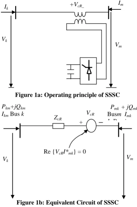
[image:3.595.300.550.45.387.2]

Improved system performance is achieved through changing the parameters of power system network using the series of FACTs controllers. Enhanced reliability or security of the system and its dynamic behavior are the advantageous enjoyed using FACTs devices. Controlling the transmission lines during power flows is considered to be the main role of FACTs devices [33, 34]. In modern power system control and operation, these control characteristics have played an important role in FACTs devices. Figure 1 indicates the components of SSSC device such as, a capacitor, a coupling transformer and an inverter. Using a coupling transformer line, the power transmission lines are connected in series altogether with SSSC device. Usually, the reactance or impedance changes in the transmission line can be regulated through inserting or generating a series voltage using SSSC device. Likewise, the point at which the connection of SSSC is made can be used to control effectively the bus voltage or transmission line flows [35].

[image:3.595.60.280.281.613.2]

Figure 1a: Operating principle of SSSC

Figure 1b: Equivalent Circuit of SSSC

The equivalent circuit of SSSC is as shown in the Figure 1b. From the equivalent circuit the power flow constraints of the SSSC can be given as

))

sin(

)

cos(

(

)

sin

cos

(

2 cR k km cR k km cR k km km km km m k kk k km

b

g

V

b

g

V

g

V

P















(5)

))

cos(

)

sin(

(

)

cos

sin

(

2 cR k km cR k km cR k km km km km m k kk k km

b

g

V

b

g

V

b

V

Q











(6)

))

sin(

)

cos(

(

)

sin

cos

(

2 cR m km cR m km cR m mk km mk km m k mk m mk

b

g

V

b

g

V

g

V

P















(7)

))

cos(

)

sin(

(

)

cos

sin

(

2 cR m km cR m km cR m mk km mk km m k mm m km

b

g

V

b

g

V

b

V

Q











(8) where km kk km kk cR km

km

mb

Z

g

b

g





1 /

,



,



km m m km

m m

g

b

g



,



Operating constraint of the SSSC (active power exchange via the DC link) is as

*

Re(

)

0 (

cos(

)

sin(

))

(

cos(

)

sin(

))

0

cR mk

k cR km k cR km k cR

m cR km m cR km m cR

PE

V I

or

V V

g

b

V V

g

b













₍₉₎

The active power flow constraint is

0

specified

mk mk

P



P



₍₁₀₎

0

specified

mk mk

Q



Q



₍₁₁₎

Where specified mk

P

Is specified active power flow.

The equivalent voltage injection

V

_cR





_cR bound constraints

are as

min max

cR cR cR

V



V



V

₍₁₂₎

max min cR cR

cR





(13)

IV. STATIC SECURITY INDEX (SSI)

From the past decades, a rapid growth is evident with the usage of fuzzy logic applications. Reasoning modes can be applied effectively using fuzzy logic (FL). Instead numbers, the words are considered to define the mapping rule of fuzzy logic. Tolerance and impression are explored using the words computed by the FL. Furthermore, the output and input spaces can be mapped effectively using FL. Nonetheless, the multi-output and multi-input systems are modeled accurately using FL tool.

Figure 2: Parallel operated fuzzy inference systems In the literature, different types of objective functions were used for optimization of power system operation. But, no one has evaluated the impact of the optimization of a particular objective function on the power system severity/security. Therefore, in order to evaluate the impact of optimization of power system operation, a fuzzy logic composite criteria based severity index is proposed in this case. Using this FL based static severity index, the

impact on network contingency ranking is also evaluated.

Vk

Pkm+jQkm

Ikm Bus k

Pmk + jQmk

Busm Imk Iij Bus i

VcR

+

ZcR

Vm

Re {VcRI*mk} = 0

Ik

Vk

+VcR_ Im

[image:3.595.313.544.517.635.2]

(4)

Adaptive Unified Differential Evolution Algorithm for Optimal Operation of Power Systems with Static

Security, Transient Stability and SSSC Device

FL based static security/severity index: As indicated in Fig

2, the parallel operated fuzzy inference systems (FIS) has adopted the severity index to obtain the total fuzzy logic composite criteria. For contingency, the static severity index is computed. When compared to the pre-fixed value, the severity index showing higher value is ranked after listing out [36].

V. OPF PROBLEM FORMULATION

Formulation of transient stability constrained standard OPF problem is as follows:

Min

f

(

u,

x

)

(14)

Subject to

g

(

u,

x

)



0

(15)

0 )

(

u,

x



h

(16)

Here, the control variables vector is indicated as

u

and the variable that corresponds to the dependent variable vector is indicated as

x

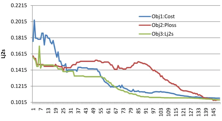
, respectively.

Objective functions: Three different forms of objective

functions included in the OPF problem are as follows: Objective Function I :

Min

f

₁=

F

_T







a

_i

P

_gi2



b

_i

P

_gi



c

_i



is the cost of generation

Objective Function II :

Min

f

₂ =

Ploss

=



 





) , ( 2 2

)

cos

2 (

j i k N k ij j i j i k l

V

g



,

is the power loss

Objective Function III :

Min

f

₃ =

Lj s

2

=



  nb g j j

L

1 2

is the

sum of squared voltage stability indices

Constraints: The OPF problem constraints are categorized

into two forms:

Equality Constraints: These constraints represent the sets of

nonlinear equations for power flows, which means,

0 )

cos(

1









 j ij ij i j

n

j i Di

Gi

P

V

Y

P





(17)

0 )

sin(

1













 j ij ij i j

n

j i Di

Gi

Q

V

Y

Q





(18)

where

P

_Gi and

Q

_Giare the real and reactive power outputs

injected at bus

i

respectively, the load demand at the same

bus is represented by

P

_Diand

Q

_Di, and elements of the bus

admittance matrix are represented by

Y

_ij and



_ij.

Inequality Constraints: These constraints that represent the

power system operational and security limits such as the bounds on the following:

Generators real and reactive power outputs

N

i

P

_Gimin



_Gi



_Gimax

,



1 ,



,

(19)

N

i

Q

_Gimin



_Gi



_Gimax

,



1 ,



,

(20) Voltage magnitudes at each bus in the network

NL

i

V

_imin



_i



_imax

,



1 ,



,

(21) Transformer tap settings

NT

i

T

i i i

,

1 ,

,

max

min





_

(22)

Reactive power injections due to capacitor banks

CS

i

Q

Ci Ci Ci

,

1 ,

,

max

min





_

(23)

Transmission lines loading

nl

i

S

_i



_imax

,



1 ,



,

(24) Voltage stability index:

NL

j

L

_j



max_j

,



1 ,



,

(25) FACTS device constraint:

min max

cR cR cR

V



V



V

SSSC voltage magnitude

(26a)

min max

cR cR cR











SSSC voltage angle

(26b) Transient stability constraint

⃒𝛿

𝑖

− 𝛿

𝐶𝑂𝐼

⃒

𝑚𝑎𝑥

≤ 𝛿

𝑚𝑎𝑥

𝑖

= 1….Ng, (27)

A system maintaining stability followed with contingency „k‟ is implied using the transient stability associated constraints as indicated in Equation (27). Power system ability is indicated using the term Transient stability index (TSI), which can be used to return back a new stable equilibrium by maintaining itself in its stable domain.

Transient stability constraints: Wide scopes of algebraic

equations are used to explain the transient stability problem of power system. For the generator, the oscillation equations derived are as follows:

𝛿

𝑖=

𝑤

𝑖

− 𝑤

0 i=1…

𝑁

𝑔 (28)

𝑀

𝑖

𝜔

= 𝜔

𝑖 0

(𝑃

𝑚𝑖

− 𝑃

𝑒𝑖

− 𝐷

𝑖

𝜔

𝑖

)

(29)

Here, the synchronous speed is indicated as

𝜔

_𝑜, for the

𝑖

𝑡𝑕 generator, the electrical output power is denoted as

𝑃

𝑐𝑖,

mechanical input power as

𝑃

_𝑚𝑖, damping constant as

𝐷

_𝑖, moment of inertia as

𝑀

_𝑖, rotor speed as

𝜔

_𝑖, and rotor angle as

𝛿

𝑖, respectively.

Likely, the center of inertia (COI) position is expressed as follows:

𝛿

𝐶𝑂𝐼 =

𝑀𝑖𝛿𝑖 𝑁 𝑔 𝑖=1

𝑀𝑖 𝑁 𝑔 𝑖=1

. (30)

Equation (31) indicates the formulation of transient stability‟s inequality constraints.

⃒𝛿

𝑖

− 𝛿

𝐶𝑂𝐼

⃒

𝑚𝑎𝑥

≤ 𝛿

𝑚𝑎𝑥

𝑖

= 1….Ng, (31)

For the

𝑖

𝑡𝑕 generator, the rotor angles maximum deviation from the COI is indicated as

⃒𝛿

_𝑖

− 𝛿

_𝐶𝑂𝐼

⃒

_𝑚𝑎𝑥 and based on the experience the maximum value allowed by the rotor angle is denoted as

𝛿

𝑚𝑎𝑥. In this study, the trial and error method is

used to determine the value of

𝛿

_𝑚𝑎𝑥. Most of the past literal works have shown different values for each system.

Fitness value computation: To the fuel cost, the state variables violations are added to determine the fitness value of an individual. Normally, using Newton-Raphson algorithm, the fuel cost value is evaluated. Consequently, for each solution, the fitness value is evaluated as follows:

ƒ 𝑥, 𝑢 = ƒ

𝑖 +

𝐾

𝑄

(𝑄

𝑔𝑖

− 𝑄

𝑔𝑖𝑙𝑖𝑚

)

2 𝑁𝑔

𝑖=1

+ 𝐾

𝑉

(𝑉

𝑖

−

𝑁𝑝𝑞 𝑖=1

𝑉𝑖𝑙𝑖𝑚)2

+

𝐾𝑠𝑖=1𝑁𝑙(𝑆𝑙− 𝑆𝑙𝑙𝑖𝑚)2

+

𝐾

_𝐿 𝑁_𝑖=1𝑝𝑞

(𝐿

_𝑗

− 𝐿

_𝑗𝑙𝑖𝑚

)

2 +

𝐾

_𝑇 𝑁_𝑖=1𝑔

(|

𝛿

_𝑖

− 𝛿

_𝐶𝑂𝐼

|

_𝑚𝑎𝑥

−

𝛿

𝑙𝑖𝑚

₎

2_.

(5)

𝑄

_𝑔𝑖𝑙𝑖𝑚 ,

𝑉

_𝑖𝑙𝑖𝑚 ,

𝑆

_𝑖𝑙𝑖𝑚 ,

𝐿

_𝑗𝑙𝑖𝑚, and

𝛿

_𝑖𝑙𝑖𝑚 are defined as follows:

𝑄

𝑔𝑖𝑙𝑖𝑚 =

𝑄

𝑔𝑖𝑚𝑎𝑥

; 𝑄

𝑔𝑖

> 𝑄

𝑔𝑖𝑚𝑎𝑥

𝑄

_𝑔𝑖𝑚𝑖𝑛

; 𝑄

𝑔𝑖

< 𝑄

𝑔𝑖𝑚𝑖𝑛

. (33a)

𝑉

𝑖𝑙𝑖𝑚 =

𝑉

_𝑖𝑚𝑎𝑥

; 𝑉

𝑖

> 𝑉

𝑖𝑚𝑎𝑥

𝑉

𝑖𝑚𝑖𝑛

; 𝑉

𝑖

< 𝑉

𝑖𝑚𝑖𝑛

. (33b)

𝐿

𝑗𝑙𝑖𝑚 =

𝐿

𝑗𝑚𝑎𝑥

; 𝐿

𝑗

> 𝐿

𝑗𝑚𝑎𝑥

𝐿

𝑗𝑚𝑖𝑛

; 𝐿

𝑗

< 𝐿

𝑗𝑚𝑖𝑛

. (34)

𝑆

_𝑙𝑙𝑖𝑚 =

𝑆

𝑙

𝑚𝑎𝑥

_{; 𝑆}

𝑙

> 𝑆

𝑙𝑚𝑎𝑥

𝑆

𝑙𝑚𝑖𝑛

; 𝑆

𝑙

< 𝑆

𝑙𝑚𝑖𝑛

. (35)

𝛿

𝑖𝑙𝑖𝑚 =

𝛿

𝑚𝑎𝑥

; ⃒𝛿

𝑖

− 𝛿

𝐶𝑂𝐼

⃒

𝑚𝑎𝑥

> 𝛿

𝑚𝑎𝑥

0: ⃒𝛿

𝑖

− 𝛿

𝐶𝑂𝐼

⃒

𝑚𝑎𝑥

< 𝛿

𝑚𝑎𝑥

. (36)

Here, the fitness function is indicated as

𝑓(𝑥, 𝑢)

. The transient stability limit, load bus voltage, the generator bus reactive power output, the slack bus reactive power output are indicated as

𝐾

_𝑇 ,

𝐾

_𝐿,

𝐾

_𝑠,

𝐾

_𝑉 and

𝐾

_𝑄, respectively. For the related variables, their upper or lower limits violations are indicated as

𝑄

_𝑖𝑙𝑖𝑚,

𝑉

_𝑖𝑙𝑖𝑚 ,

𝑆

_𝑙𝑙𝑖𝑚 and

𝐿

_𝑗𝑙𝑖𝑚, respectively. The number of load buses is indicated as

𝑁

_𝑝𝑞, respectively. The penalty value is assumed to be zero when, the constraints relay within their lower and upper limits

VI. STANDARD DIFFERENTIAL EVOLUTION Population initialization is the first step of DE algorithm. Initial population is formed through random generation of NP solutions group included in the control parametric space. Update of population from one cycle to the next cycle is performed soon after completing the initialization step. When reached maximum number of cycles, the repetition of process is stopped; otherwise, the process is continued until the termination criterion is attained. However, the mutation, crossover, and selection are the three kinds of operations used for updating the populations at each cycle or generations. Both crossover and mutation operations are applied to generate new solutions in every generation/iteration. Then, the appropriate solutions from these generated new solutions are obtained through applying the selection operation [37].

Individuals are referred to be the NP populations that are evolved using DE algorithm. In D-dimensional parametric space, the candidate solutions are encoded to achieve the

global optimum (i.e.

𝑋

_𝑖,𝐺

= 𝑋

_𝑖,𝐺1

, … . . , 𝑋

_𝑖,𝐺𝐷

, 𝑖 =

1, … . . , 𝑁𝑃

). Inside the search space, the individuals are randomized uniformly considering the maximum and minimum parametric limits

𝑋

_𝑚𝑖𝑛

= 𝑋

_𝑚𝑖𝑛1

, … . . , 𝑋

_𝑚𝑖𝑛𝐷 and

𝑋

_𝑚𝑎𝑥

= 𝑋

_𝑚𝑎𝑥1

, … . . , 𝑋

_𝑚𝑎𝑥𝐷 , respectively. For instance, at generation G=0, the

𝑖𝑡𝑕

individual containing the initial value of

𝑗𝑡𝑕

parameter is as follows:

𝑥

_𝑖,0𝑗

= 𝑥

_𝑚𝑖𝑛𝑗

+ 𝑟𝑎𝑛𝑑 0,1 ∙ 𝑥

_𝑚𝑎𝑥𝑗

− 𝑥

_𝑚𝑖𝑛𝑗

, 𝑗 =

1,2,3, … . . , 𝐷

(37)

Here, the limit [0, 1] considered for uniform distribution of random variables is indicated as

𝑟𝑎𝑛𝑑 0,1

.

Mutation Operation: Considering each individual

𝑋

_𝑖,𝐺

(target vector) in the current population, the mutant vector

𝑉

_𝑖,𝐺 is generated using the mutation operation applied by the DE algorithm after completing the initialization of population or solutions. From the below given mutation strategies, any

one of them can be selected to generate the mutant vector

𝑉

_𝑖,𝐺

= 𝑣

_𝑖,𝐺1

, 𝑣

_𝑖,𝐺2

, … . , 𝑣

_𝑖,𝐺𝐷 corresponding to each target vector

𝑋

_𝑖,𝐺 at each cycle. In DE algorithm, the commonly used mutation operation strategies are provided below:

“

𝐷𝐸/𝑟𝑎𝑛𝑑/1

”

𝑉

𝑖,𝐺

= 𝑋

_𝑟₁𝑖_,𝐺

+ 𝐹 ∙ 𝑋

_𝑟

2𝑖,𝐺

− 𝑋

𝑟3𝑖,𝐺 (38)

“

𝐷𝐸/𝑏𝑒𝑠𝑡/1

”

:

𝑉

_𝑖,𝐺

= 𝑋

_{𝑏𝑒𝑠𝑡 ,𝐺}

+ 𝐹 ∙ 𝑋

_𝑟

1𝑖,𝐺

− 𝑋

𝑟2𝑖,𝐺 (39)

“

𝐷𝐸/𝑟𝑎𝑛𝑑 − 𝑡𝑜 − 𝑏𝑒𝑠𝑡/1

”

: 𝑉

_𝑖,𝐺

= 𝑋

_𝑖,𝐺

+ 𝐹 ∙

𝑋

_{𝑏𝑒𝑠𝑡 ,𝐺}

− 𝑋

_𝑖,𝐺

+ 𝐹 ∙ 𝑋

_𝑟

1𝑖,𝐺

− 𝑋

𝑟2𝑖,𝐺 (40)

4)

“

𝐷𝐸/𝑏𝑒𝑠𝑡/2

”

:

𝑉

𝑖,𝐺

= 𝑋

𝑏𝑒𝑠𝑡 ,𝐺

+ 𝐹 ∙ 𝑋

_𝑟₁𝑖_,𝐺

− 𝑋

_𝑟

2𝑖,𝐺

+ 𝐹 ∙

𝑋

_𝑟

3𝑖,𝐺

− 𝑋

𝑟4𝑖,𝐺 (41)

5) “DE/rand/2”:

𝑉

_𝑖,𝐺

= 𝑋

_𝑟

1𝑖,𝐺

+ 𝐹 ∙ 𝑋

𝑟2𝑖,𝐺

− 𝑋

𝑟3𝑖,𝐺

+ 𝐹 ∙

𝑋

_𝑟

4𝑖,𝐺

− 𝑋

𝑟5𝑖,𝐺 (42)

Here, the indices generated are represented as

𝑟

₁𝑖

, 𝑟

₂𝑖

, 𝑟

₃𝑖

, 𝑟

₄𝑖

, 𝑎𝑛𝑑 𝑟

₅𝑖 , respectively. They are called exclusive integers generated in mutual and random manner. For each mutant vector, the random generation of these indices is performed. Vector difference is scaled using a positive control and scaling factor denoted as F. In a specific generation, the best fitness value containing individual vector is represented as

𝑋

_{𝑏𝑒𝑠𝑡 ,𝐺}.

Crossover Operation: A trial vector

𝑈

_𝑖,𝐺

=

𝑢

_𝑖,𝐺1

, 𝑢

_𝑖,𝐺2

, … . , 𝑢

_𝑖,𝐺𝐷 is generated from the mutant vector

𝑉

_𝑖,𝐺 and its relative target vector

𝑋

_𝑖,𝐺 by means of applying the crossover operation. This process is done after finishing the mutation operation. Uniform (binomial) crossover employed for the basic DE algorithm is as follows:

𝑢

_𝑖,𝐺𝑗

=

𝑣

_𝑖,𝐺𝑗

, 𝑖𝑓 𝑟𝑎𝑛𝑑

_𝑗

0,1 ≤ 𝐶𝑅 𝑜𝑟 (𝑗 = 𝑗

_{𝑟𝑎𝑛𝑑}

)

𝑥

_𝑖,𝐺𝑗

, 𝑜𝑡𝑕𝑒𝑟𝑤𝑖𝑠𝑒

𝑗 =

1,2,

…

..,𝐷.

(43) Usually, the mutant vector is observed to copy the fraction of parameter values. These values are then controlled using a significant constant called crossover rate CR relaying in the limit [0,1] (as indicated in (43). In case, if

𝑟𝑎𝑛𝑑

_𝑗

0,1 ≤

(6)

Adaptive Unified Differential Evolution Algorithm for Optimal Operation of Power Systems with Static

Security, Transient Stability and SSSC Device

Selection Operation: Best population is obtained after

employing the selection operation. Target vector

𝑓(𝑋

_𝑖,𝐺

)

is used to compare each trial vector

𝑓(𝑈

_𝑖,𝐺

)

and its relative objective function value. Compared to the target vector, the equal or less objective function value obtained by the trial vector can take place in the next cycle as an individual by replacing the target vector. If this is not the case then, the next cycle is continued with the target vector. Equation (44) indicates the selection operation.

𝑋

𝑖,𝐺+1

=

𝑈

_𝑖,𝐺

, 𝑖𝑓𝑓 𝑈

_𝑖,𝐺

≤ 𝑓 𝑋

_𝑖,𝐺

𝑋

_𝑖,𝐺

, 𝑜𝑡𝑕𝑒𝑟𝑤𝑖𝑠𝑒

(44)

After reaching the termination criterion, the repetition of the process is stopped.

VII. ADAPTIVE UNIFIED DIFFERENTIAL EVOLUTION

Standard differential evolution algorithm has been improved using the newly proposed ten various forms of mutation strategies. When quantified numerous test samples of different optimization problems, the “DE/best /1/bin” has achieved good performance compared to “DE/ rand/1 bin”. However, the ICEC96 contest has suggested using the DE/best /2/bin due to its excellent performance [38, 39]. Usage of differential evolution algorithm can cause difficulties with the existence of multiple mutation strategies. Works in [40-42] have proposed the techniques of combining different forms of multiple mutation strategies.

In this work, the differential evolution algorithm using many of the traditional mutation strategies are unified through developing a new single mutation expression. This can be expressed as follows:

𝑣

𝑖

= 𝑥

𝑖

+ 𝐹

1

𝑥

𝑏

− 𝑥

𝑖

+ 𝐹

2

𝑥

𝑟1

− 𝑥

𝑖

+

𝐹

3

𝑥

𝑟2

− 𝑥

𝑟3

+ 𝐹

4

𝑥

𝑟4

− 𝑥

𝑟5 (45)

In the current iteration (generation), the best solution identified is indicated in the right side of Eq. (45) (i.e. in second term). From the random solution, the rational invariant contributions obtained are indicated in third term [43]. As similar to the normal differential evolution algorithm, the parent solutions differences are indicated in the 4th and 5th terms.

From the best solution, the mutated solutions are diverted away using the final three terms. This helps in the improvement of exploration process of the algorithm during making decision in the parametric space. The weights

obtained are represented using four parameters such as,

F

₁,

2

F

,

F

₃and

F

₄. In order to produce a new mutant solution, the exploration and exploitation are combined using mutation expression operation. Mutation operators space is explored widely using an opportunity provided by this new expression. It is possible to achieve a new mutation strategy during

applying a differential set of parameters such as,

F

₁,

F

₂,

F

₃, and

F

₄. Compared to the most of the traditional standard differential evolution algorithms, a better optimization solution can be obtained using a unified mutation strategy.

During performing different optimization stages, various combinations of mutation strategies can be applied through adjusting the differential set of parameters at each evolution of the optimization process. Hence, the simplicity in

mathematical expressions is enjoyed in these unified mutation operations.

Different mutation strategies are used and combined using a method provided by the unified mutation strategy. Thereby, the application users have considered the selection of suitable

control parameters

F

₁,

F

₂,

F

₃, and

F

₄is a time consuming and tedious process. Performance of the algorithm is highly improved and the computational burden of the application users is reduced on selecting the control parameters using a self-adaptive method.

In past studies, a number of parameters control methods were used for the conventional differential evolution algorithm [44-48]. The proposed unified differential algorithm in this work is developed through evolving

dynamically the five control parameters

F

₁,

F

₂,

F

₃,

F

₄ and

r

C

of classical self-adaptive method. In most of the experimental tests, the good performance was achieved using this simple self-adaptive scheme.

In this study, a set of control parameters

NP

1,2,3,....

i

,

x

_i



are comprised in each individual

solution during the generation

G

of the mutation process in self-adaptive method. A new control parameter sets

𝐹

1,𝑖𝐺+1

, 𝐹

2,𝑖𝐺+1

, 𝐹

3,𝑖𝐺+1

, 𝐹

4,𝑖𝐺+1

𝑎𝑛𝑑𝐶

𝑟𝐺+1_𝑖 are computed prior to

the adaptation of unified differential evolution expressions for producing a new mutant solution.

𝐹

_{𝑗 ,𝑖}𝐺+1

=

𝐹

𝑗𝑚𝑖𝑛

+ 𝑟

𝑗 1

𝐹

𝑗𝑚𝑎𝑥

− 𝐹

𝑚𝑖𝑛

, 𝑖𝑓𝑟

𝑗 2

< 𝜏

𝑗

𝐹

_{1,𝑖𝑜𝑡 𝑕𝑒𝑟𝑤𝑖𝑠𝑒}𝐺 (46)

𝐶

𝑟𝑖

𝐺+1₌

𝐶

𝑟𝑚𝑖𝑛

+ 𝑟

3

𝐶

𝑟𝑚𝑎𝑥

− 𝐶

𝑟𝑚𝑖𝑛

, 𝑖𝑓𝑟

4

< 𝜏

5

𝐶

𝑟𝐺_{𝑖, 𝑜𝑡 𝑕 𝑒𝑟𝑤𝑖𝑠𝑒}

(47)

Maximum and minimum values of the control parameters are expressed as

𝐹

_{𝑗𝑚𝑖𝑛}

𝑎𝑛𝑑𝐹

_{𝑗𝑚𝑎𝑥} for j=1, 2, 3, 4; whereas, the uniform random values distributed in the interval [0,1] are indicated as

𝑟

_{𝑗 1}

, 𝑟

_{𝑗 2}

, 𝑗 = 1,2,3, 𝑟

₃

, 𝑟

₄ , respectively. Subsequently, the maximum and minimum cross over probability of the control parameters are denoted as

𝐶

𝑟𝑚𝑎𝑥 and

𝐶

𝑟𝑚𝑖𝑛 . For the

𝑗

𝑡𝑕 _{control parameter, the}

probability of old value and new value used is indicated as

𝜏

𝑗

,

j=1, 2,3,4,5. Notably, it is important to maintain the value

of

𝜏

_𝑗 to be smaller for further generating the new trial solutions by means of reusing the survived solutions. In this work, the value of

𝜏

𝑗 is fixed to 0.1. Also, the values 0 and 1

are fixed to

𝐹

_{𝑗𝑚𝑖 𝑛}

𝑎𝑛𝑑𝐹

_{𝑗𝑚𝑎𝑥} , respectively. The control parameters values are fixed to

𝐶

_𝑟

𝑚𝑎𝑥=1 and

𝐶

𝑟𝑚𝑖𝑛 =0. Based

on different traditional mutation strategies, the values for these parameters are selected. However, the mutant solution is generated using this new control parameter step. In between the minimum and maximum values, the initial values for the control parameters are assigned. Pseudo-code of the AuDE algorithm is indicated below as follows:

Pseudo-code of AuDE algorithm: Based on uniform

samplings distributed randomly in the interval [0,1], the initial control parameters

𝐹

₁

, 𝐹

₂

, 𝐹

₃

, 𝐹

₄

, 𝐶

_𝑟 are generated. The NP points are sampled randomly inside the feasible control parametric space

𝑥

to generate a set of initial population. Then, their

(7)

function values f(x) are evaluated. Initialize the generation number as G=0 While not attained the stopping criteria, Do: For i=1to NP (for each parent solutions target

𝑥

_𝑖): Mutation

Determine a set of control parameters (for j=1, 2, 3, and 4):

𝐹

_{𝑗 ,𝑖}𝐺+1

=

𝐹

𝑗𝑚𝑖𝑛

+ 𝑟

𝑗 1

𝐹

𝑗𝑚𝑎𝑥

− 𝐹

𝑚𝑖𝑛

, 𝑖𝑓𝑟

𝑗 2

< 𝜏

𝑗

𝐹

1,𝑖𝑜𝑡 𝑕𝑒𝑟𝑤𝑖𝑠𝑒𝐺

𝐶

𝑟𝑖

𝐺+1₌

𝐶

𝑟𝑚𝑖𝑛

+ 𝑟

3

𝐶

𝑟𝑚𝑎𝑥

− 𝐶

𝑟𝑚𝑖𝑛

, 𝑖𝑓𝑟

4

< 𝜏

5

𝐶

𝑟𝐺_{𝑖, 𝑜𝑡 𝑕 𝑒𝑟𝑤𝑖𝑠𝑒}

Using AuDE mutation strategy to determine a mutant solution vector:

𝑣

𝑖

= 𝑥

𝑖

+ 𝐹

1𝐺+1

𝑥

𝑏

− 𝑥

𝑖

+ 𝐹

2𝐺+1

𝑥

𝑟1

− 𝑥

𝑖

+ 𝐹

3𝐺+1

𝑥

𝑟2

− 𝑥

𝑟3

+ 𝐹

4𝐺+1

𝑥

𝑟4

− 𝑥

𝑟5

Crossover

Generate a new trial solution

𝑈

𝑖(

𝑢

𝑖1

, 𝑢

𝑖2

, … … .. … , 𝑢

𝑖𝐷

)

through binomial crossover scheme:

𝑢

𝑖𝑗=

𝑢

𝑖𝑗 if

𝑟𝑎𝑛𝑑

𝑖𝑗[0,1]

≤ 𝐶

𝑟𝑖

𝐺+1_{or j=}

_𝑗

𝑟𝑎𝑛𝑑 ,

Otherwise

𝑢

𝑖𝑗

= 𝑥

𝑖𝑗

Selection

For the trial solution

𝑓(𝑈

_𝑖

)

compute the objective functions If

𝑓(𝑈

𝑖

) ≤ 𝑓(𝑥

𝑖

)

then

𝑥

𝑖,𝐺+1

= 𝑈

𝑖

Else

𝑥

_𝑖,𝐺+1

= 𝑥

_𝑖,𝐺 Find For

G=G+1 End While

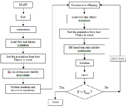
VIII. IMPLEMENTATION OF AUDE ALGORITHM FOR OPF PROBLEM

Number of populations

(N

_p

)

is significantly adopted by the natural evolution algorithm called differential evolution to attain an optimal solution through repeating the iterations. In this section, the adaptive unified differential evolution algorithm is applied to solve TSCOPF problem. Initialization, selection, and evaluation of solutions are the three most important strategies introduced by the differential evolution algorithm (DEA). However, these strategies mainly aimed for the minimization of computational time. The flow chart of the proposed AuDE algorithm for solving the TSCOPF problem is illustrated in Fig.3. Detailed explanation is provided in this section.

Using individuals (populations) to encode the control

variables: In order to withstand the TSCOPF issues, the

differential algorithm should be applied only after identifying the number of control variables from the problem that are

need to be optimized. Here,

Q

_ciindicates the shunt reactive power,

T

_ti as tap changing transformers,

V

_gi as voltage magnitudes generator, and

P

_g1is the slack unit not considered

in

P

_giknown as the outputs of the active power generator. Therefore, u can be expressed as

𝑢

𝑇= [

𝑃

_𝑔2, . . . .

𝑃

_𝑔𝑁𝑔,

𝑉

_𝑔1, . . . .

𝑉

_𝑔𝑁𝑔,

𝑇

_𝑡1, . . . .

𝑇

_𝑡𝑁𝑡,

𝑄

_𝐶1, . . . .

𝑄

_𝐶𝑁𝑐] (48)

Selecting the size of population:- Problem size is adopted

for accurate selection of the population size

(N

_p

)

.

Considering C as the control variables in most of the real world engineering problems, then obtaining optimal

solutions with

N

p



2 C

is a complex process and easier with

N

_p



20 C

condition [49]. Furthermore, the possible optimal solutions are obtained using the population size

C

5

3 N

_p





In AuDE algorithm, the populations are initialized through employing the OBL scheme. This process is done to improve the solution quality [50].

Based on Eq. (49), an individual

u

containing the control variables are generated randomly within a specific limit. However, the first iteration has used these randomly generated individuals as the root (parent) population.

𝑢

_𝑖,𝑗0 =

𝑟𝑎𝑛𝑑 0,1 ∗ 𝑢

_𝑗𝑚𝑎𝑥

−𝑢

_𝑗𝑚𝑖𝑛

+ 𝑢

_𝑗𝑚𝑖𝑛 (49)

0 min max

, ,

i j j j i j

ou



u



u



u

//opposition-based learning

Selecting

𝑁

_𝑃 fittest individuals from set the {

𝑢

_𝑖,𝑗0 ,

𝑜𝑢

_𝑖,𝑗0 } as initial population;

At the kth generation, the control variables

j

in a population

i

is indicated as

u

k_i,_j representing

}

N

.,

{1,2,3,...

i



p and

j



{1,2,3,...

.,

N

p

}

, respectively.

For the control variable

j

, their upper and lower limits are

indicated as

u

min_j and

u

max_j .

Below said procedures are followed for satisfying the

constraints in slack bust active power. Consider

P

_Las the total active load of the system,

P

_dsbe the power summed through not including the slack unit as well as dispatching from all the generators. Subsequently, the slack bus generator active power is assigned with a value obtained by means of

subtracting

P

_ds from

P

_L. In case, if the slack bus generators upper or lower limits are exceeded by the value assigned to

the slack bus active power, then the limits

P

_slackmaxor

P

_slackminare fixed to its active power. The other generators are assigned with the residual active power, proportionally.

Implementing load flow technique: In order to compute the

power flow solutions, the Newton-Raphson power flow program is implemented for each population (individual). Indices of voltage stability, line flows, load bus voltages, outputs of the reactive power are considered as the constraints of power system operation. These constraints are verified and the slack bus (independent generator) generations are calculated during evaluating the power flow solutions.

Fitness Computation: Each individual‟s quality can be

measured by evaluating every individual solution using

penalty functions included in the fitness measure

F

_i as shown below:

𝐹

_𝑖

=

1 (𝑓

_𝑖

+ K

_Q

F

_Qi

+ K

_v

F

_Vi

+ K

_S

F

_Si

+ K

_L

F

_Li

+ K

_T

F

_Ti

)

(8)

Adaptive Unified Differential Evolution Algorithm for Optimal Operation of Power Systems with Static

Security, Transient Stability and SSSC Device

𝐹

_𝑄𝑖= 𝑁_𝑙=1𝑔

(|𝑄

_𝐺𝑖𝑙

− 𝑄

_𝐺𝑖𝑙𝑙𝑖𝑚

|)

2 (51a)

𝐹

𝑉𝑖=

(|𝑉

𝑖𝑙 𝑁𝑝𝑞

𝑙=1

− 𝑉

𝑖𝑙𝑙𝑖𝑚

|)

2 (51b)

𝐹

_𝑆𝑖= 𝑁𝑙_𝑙=1

(|𝑆

_𝑙𝑖

− 𝑆

_𝑙𝑖𝑙𝑖𝑚

|)

2 (53a)

𝐹

_𝐿𝑖= 𝑁𝑝𝑞_𝑙=1

(|𝐿

_𝑗

− 𝐿

_𝑗𝑙𝑖𝑚

|)

2 (53b)

𝐹

_𝑇𝑖

=

𝑁_𝑖=1𝑔

(|

𝛿

𝑖

− 𝛿

𝐶𝑂𝐼

|

_𝑚𝑎𝑥

− 𝛿

𝑙𝑖𝑚

)

2 (54)

Here, the fuel costs

(f

_i

)

generated by the system is represented as

F

_Qi,

F

_Vi ,

F

_Si,

F

_Liand

F

_{T i}, respectively. For each individual

i

, the outputs of reactive power generators corresponding normalized violations summations, rotor angles generator, voltage stability indices, and PQ-bus voltages are also shown in Eq. (54)

𝑁

_𝑝𝑞 is the total number of PQ buses,

𝑁

_𝑔 is the total number of generator,

𝑁

_𝑙is the total number of lines;

𝑄

_𝑔𝑖𝑙𝑙𝑖𝑚,

𝑉

_𝑖𝑙𝑙𝑖𝑚,

𝑆

_𝑖𝑙𝑙𝑖𝑚,

𝐿

_𝑗𝑖𝑙𝑙𝑖𝑚and

𝛿

𝑙𝑖𝑚denote the violated upper and lower limits of the generator reactive power outputs, voltages of the load buses, line flows, voltage stability indices of load buses and generator rotor angle respectively;

K

_Q ,

K

_v

K

_S

K

_L and

K

_T are the corresponding penalty coefficients. Ultimately, if obtained higher the fitness value, then better the individual is generated.

Assessment of transient stability: Actually, the TSCOPF

optimization problems have large searching space; thereby, it is a time-consuming process to assess the transient stability constraints. Hence, during TSA computation process, the populations (individuals) with good fitness alone are allowed to determine the stable and feasible optimal solutions. This process has reduced the computational burden by not delimiting the evolutions reproduction abilities. By the fact, the fitness function has included in the transient stability to satisfy its conditions neither for satisfying the optimization objectives. Therefore, before going to the evaluation of transient stability, each individual is evaluated for the SSI values whose value is less than or equal to the specified value. During evolution, the selection process will be maintained effectively through handling the system stability in a chosen contingency using that specific individual.

Global best individual: From all generations, the best

individual obtained is indicated as

𝑢

_{𝑏𝑒𝑠𝑡}(i.e. the global best individual). To find

𝑢

_{𝑏𝑒𝑠𝑡} individuals, two individuals

𝑢

_𝑎 and

𝑢

_𝑏are compared in a particular generation,

𝑢

_𝑎 is defined” better” than

𝑢

𝑏 if matched any one of the below

given criterions:

Higher fitness value is for

u

_aand both of them are stable Higher fitness value is for

u

_aand both of them are unstable Instability is for

u

_band stability for

u

_a

Mutation operation: Different evolution algorithms that

have used few traditional mutation strategies are unified with the aid of a single mutation expression. This is expressed as follows:

𝑣

𝑖

= 𝑥

𝑖

+ 𝐹

1𝐺+1

𝑥

𝑏

− 𝑥

𝑖

+ 𝐹

2𝐺+1

𝑥

𝑟1

− 𝑥

𝑖

+

𝐹

3𝐺+1

𝑥

𝑟2

− 𝑥

𝑟3

+ 𝐹

4𝐺+1

𝑥

𝑟4

− 𝑥

𝑟5 (55)

In order to produce a new mutant solution, the exploration and exploitation are combined using mutation expression operation. Mutation operators space is explored widely using

an opportunity provided by this new expression. It is possible to achieve a new mutation strategy during applying a

differential set of parameters such as,

F

₁,

F

₂,

F

₃, and

F

₄. Compared to the most of the traditional standard differential evolution algorithms, a better optimization solution can be obtained using a unified mutation strategy.

At the time of performing different optimization stages, various combinations of mutation strategies can be applied through adjusting the differential set parameters during each evolution of the optimization process. Hence, the simplicity in mathematical expressions is enjoyed in these unified mutation operations. The proposed unified differential algorithm in this work is developed through evolving

dynamically the five control parameters

F

₁,

F

₂,

F

₃,

F

₄ and

r

C

of classical self-adaptive method. In most of the experimental tests, the good performance was achieved using this simple self-adaptive scheme.

In this study, a set of control parameters

NP

1,2,3,....

i

,

x

_i



are comprised in each individual

solution during the generation

G

of the mutation process in self-adaptive method. A new control parameter sets

𝐹

_1,𝑖𝐺+1

, 𝐹

_2,𝑖𝐺+1

, 𝐹

_3,𝑖𝐺+1

, 𝐹

_4,𝑖𝐺+1

𝑎𝑛𝑑𝐶

𝑟𝐺+1_𝑖 are computed prior to

the adaptation of unified differential evolution expressions for producing a new mutant solution.

𝐹

𝑗 ,𝑖𝐺+1

=

𝐹

𝑗𝑚𝑖𝑛

+ 𝑟

𝑗 1

𝐹

𝑗𝑚𝑎𝑥

− 𝐹

𝑚𝑖𝑛

, 𝑖𝑓𝑟

𝑗 2

< 𝜏

𝑗

𝐹

_{1,𝑖𝑜𝑡 𝑕𝑒𝑟𝑤𝑖𝑠𝑒}𝐺 (56)

𝐶

𝑟𝑖

𝐺+1₌

𝐶

𝑟𝑚𝑖𝑛

+ 𝑟

3

𝐶

𝑟𝑚𝑎𝑥

− 𝐶

𝑟𝑚𝑖𝑛

, 𝑖𝑓𝑟

4

< 𝜏

5

𝐶

𝑟𝑖, 𝑜𝑡 𝑕 𝑒𝑟𝑤𝑖𝑠𝑒

𝐺 (57)

Maximum and minimum values of the control parameters are expressed as

𝐹

_{𝑗𝑚𝑖𝑛}

𝑎𝑛𝑑𝐹

_{𝑗𝑚𝑎𝑥} for j=1, 2, 3, 4; whereas, the uniform random values distributed in the interval [0,1] are indicated as

𝑟

_{𝑗 1}

, 𝑟

_{𝑗 2}

, 𝑗 = 1,2,3, 𝑟

₃

, 𝑟

₄ , respectively. Subsequently, the maximum and minimum cross over probability of the control parameters are denoted as

𝐶

𝑟_𝑚𝑎𝑥 and

𝐶

𝑟_𝑚𝑖𝑛 . For the

𝑗

𝑡𝑕 control parameter, the

probability of old value and new value used is indicated as

𝜏

𝑗

,

j=1, 2,3,4,5. Notably, it is important to maintain the value

of

𝜏

_𝑗 to be smaller for further generating the new trial solutions by means of reusing the survived solutions.

Crossover Operation: A trial vector

𝑈

_𝑖,𝐺

=

𝑢

_𝑖,𝐺1

, 𝑢

_𝑖,𝐺2

, … . , 𝑢

_𝑖,𝐺𝐷 is generated after performing the mutation operation. In other words, this trial vector is generated through applying crossover operation to the mutant vector

𝑉

_𝑖,𝐺 and to its target vector pairs

𝑋

_𝑖,𝐺. Uniform (binomial) crossover is employed to the AuDE as follows:

𝑢

_𝑖,𝐺𝑗

=

𝑣

_𝑖,𝐺𝑗

, 𝑖𝑓 𝑟𝑎𝑛𝑑

𝑗

0,1 ≤ 𝐶𝑅 𝑜𝑟 (𝑗 = 𝑗

𝑟𝑎𝑛𝑑

)

𝑥

_𝑖,𝐺𝑗

, 𝑜𝑡𝑕𝑒𝑟𝑤𝑖𝑠𝑒

𝑗 =

1,2,

…

..,𝐷.

(58)

In case, if

𝑟𝑎𝑛𝑑

_𝑗

0,1 ≤ 𝐶𝑅

or

𝑗 = 𝑗

_{𝑟𝑎𝑛𝑑} then to the trial vector element

𝑈

_𝑖,𝐺 , the mutant vectors

𝑉

_𝑖,𝐺 jth parameter is copied by the

(9)

corresponding target vector

𝑋

_𝑖,𝐺 is considered to copy the jth mutant vector parameter. Also, considering the target vector

𝑋

_𝑖,𝐺, the trial vectors

𝑈

_𝑖,𝐺 residual parameters are copied. Condition

𝑗

_{𝑟𝑎𝑛𝑑} ensures that the trial vector

𝑈

_𝑖,𝐺 will be different from its corresponding target vector

𝑋

_𝑖,𝐺 by at least one parameter.

Verifying the boundary limits: During evaluating the

evolutionary based optimization algorithms, their unavoidable constraints are handled in numerous ways. In case, if any of the individual element in the AUDE algorithm drops its corresponding inequality constraints, then the minimum/maximum operating point is fixed based on the individual position.

Analysis of power flow to offspring individuals: Each

[image:9.595.64.278.311.492.2]

offspring individuals power flow solutions are computed using a Newton-Raphson power flow program. The slack bus generators corresponding generations are calculated during this process. Then, the fitness function is evaluated through verifying the constraints of power system operation (voltage stability indices, line flows, load bus voltages, and reactive power outputs).

Figure 3: Flow chart for solution of TS-OPF problem

Transient stability assessment: By the fact, the fitness

function has included in the transient stability to satisfy its conditions neither for satisfying the optimization objectives. Therefore, before going to the evaluation of transient stability, each individual is evaluated for the SSI values whose value is less than or equal to the specified value. During evolution, the selection process will be maintained effectively through handling the system stability in a chosen contingency using that specific individual.

Selection: A “one- to-one” selection process actually

indicates this selection scheme. Ultimately, the best

individual is selected by comparing the parent individual

𝑢

_𝑖𝑘 to its offspring individual

𝑢

′

𝑘

. In the next generation, the parent population was obtained from the previous updated population of generation „k‟ (i.e. the selected individuals).

Updating the global best individual: From the generation k,

the updated population‟s best individuals are determined and denoted as 𝑢𝑏𝑒𝑠𝑡𝑘 . When compared to 𝑢𝑏𝑒𝑠𝑡, if found the better one is 𝑢𝑏𝑒𝑠𝑡𝑘 then, using 𝑢𝑏𝑒𝑠𝑡𝑘 the term 𝑢𝑏𝑒𝑠𝑡 is replaced.

Verifying end condition: The iteration process is repeated

continuously until the end condition is attained. In this work, after satisfying the given criterion, the iteration of AuDE is

stopped: At any time a pre-determined generations are achieved, then it is possible to stop the optimization process.

IX. SIMULATION RESULTS

The IEEE test systems such as, 39-bus, New England ten-generator, and 30-bus, six-generator systems are used to test the effectiveness of proposed AuDE method. Constant impedance models of the loads and synchronous generators are modeled using the traditional generator model. Here, the simulation period is fixed to 2.0s and transient stability simulation is performed using 0.01s as integration time step. Reliability and robustness of the proposed AuDE method is verified through performing 20 trial runs for each test case. Implementation is done using MATLAB 7.8 software. The hardware components adopted for implementation are 2.0GB RAM PC, and Intel Core 2 Duo of 2 GHz.

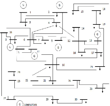
A. Results of IEEE 30-bus system

The 30-bus test system consists of a transmission network of 41 branches with interconnection of six generating units as shown in Fig. 4. However, the total real and reactive power loads in the transmission network is 283.4 MW and 126.2 MVAR respectively. Ref. [51] is used to obtain the branch and bus data. Here, off-nominal tap ratio is included in 4 transformers. For buses 10, 12, 15, 17, 20, 21, 23, 24 and 29, the shunt injections are applied. In this work, the swing bus is assumed to be bus 1. Also, it is used to consider the real power generations with its minimum and maximum limits, and cost coefficients [51]. The value 0.9 and 1.1 pu is fixed to be the minimum and maximum limits of the control variables of tap changing transformer. Conversely, the value 0.9 and 1.1 pu is fixed to be the minimum and maximum limits of voltages of generators. For load buses, their minimum and maximum voltages used are 0.95 and 1.1, respectively. Ref [52] is used to fix the limits of line flows.