Post-test implementation of TWNTN4A correction code at O.3m TCT

(1)

Rochester Institute of Technology

RIT Scholar Works

Theses

Thesis/Dissertation Collections

2001

Post-test implementation of TWNTN4A

correction code at O.3m TCT

Ryuichi Machida

Follow this and additional works at:

http://scholarworks.rit.edu/theses

This Thesis is brought to you for free and open access by the Thesis/Dissertation Collections at RIT Scholar Works. It has been accepted for inclusion in Theses by an authorized administrator of RIT Scholar Works. For more information, please [email protected].

Recommended Citation

(2)

Post-Test Implementation of

TWNTN4A Correction Code at O.3m TCT

by

Ryuichi Machida

A Thesis Submitted in

Partial Fulfillment of the

Requirement for the

MASTER OF SCIENCE

IN

MECHANICAL ENGINEERING

Approved by:

Dr. Amitabha Ghosh

Department of Mechanical Engineering

Dr. P. Venkataraman

Dr. Kevin B. Kochersberger

Dr. Satish G. Kandlikar

(Thesis Advisor)

(Graduate Committee)

(Department Head)

(3)

Permission from Author Required

Thesis Title:

Post-Test Implementation of

TWNTN4A Correction Code at O.3m TCT

I, Ryuichi Machida, prefer to be contacted each time a request for reproduction is made.

If

permission is granted, any reproduction will not be for commercial use or profit. Also,

passages in this volume must not be copied or closely paragraphed without a written

permission from the author.

If

a reader obtains any assistance from this volume, he/she must

give a proper credit in his/her own work. I can be reached at the following e-mail addresses:

(4)

Table

of

Contents

Content PageNumber

Abstract i

Acknowledgement ii

ListofFigures iii

ListofTables iv

Listof

Symbols, Subscripts,

& Abbreviations v~_vi

Chapter 1 - Introduction 1-7

Chapter 2- TWNTN4A

Theory

8-14

Chapter3- Numerical Procedure 15-24

Chapter4 - Semi-Automation 25-29

Chapter5- Results 30-55

Chapter 6

-Concluding

Remarks 56-58

References R1-R2

(5)

Abstract

Airfoil characteristics measured in a wind tunnel

typically

differ fromthose obtainedin free

airdueto the confinement of airflowin tunnel testsections andthedevelopmentof

boundary

layer on tunnel walls. Wind tunnel measured _quantities, e.g. Mach number, Reynolds

number, angle of _attack, require corrections todetermine their equivalent values in free air.

TWNTN4A is a correction program capable of _correcting wall interference effects in 2-D

wind tunnels. TWNTN4A was applied to correct over 300 data files obtained from tests

performed in 0.3m Transonic Cryogenic Tunnel

(TCT)

at NASA Langley. Data describe

Mach number range of 0.50 ~

0.82,

angle of attack ~

13,

_and Reynolds _number

3,000,000 and9,000,000. Asa new

feature,

variable grid control has been introducedto the

correction code, and semi-automatic procedure wasdeveloped toachieve volume _processing

of experimental data files. Mostof the corrected results correlated well with an interference

free viscous numerical solution given

by

Swanson/Turkel.

However,

results from variable

grid control questionedthe_validityof numerical scheme usedfor lower Mach number cases

(M =_0.50 ~

(6)

Acknowledgement

Many

havesupported and encouraged me to make this thesis possible. Special thanks goto

my parents (Motohiro and

Yoko)

and _{my brother}

(Yoshimasa)

for

helping

me in all the

possible ways

they

could. I want to thank _my advisor, Dr. Amitabha

Ghosh,

for his helpful

advice and_givingmedirectionstocomplete this thesis. Ialso wantto thank theentire

faculty

and staffinmechanical _engineering atR.I.T. fortheirsupport. Special thanksgotoall of_my

friends from Roberts Wesleyan College and mechanical _{engineering department} at R.I.T.

Their

friendship

has made _{my study in} the U.S. possible and successful.

Finally,

I want to thankRolfOrsagh atImpact

Technologies,

LLC _{for reviewing} this thesis and all the people

(7)

List

of

Figures

Figure Title Page

1.1

2.1 2.2

2.3

3.1

3.2

3.3

4.1

5.1

5.2

5.3

5.4

5.5 5.6

5.7

5.8 5.9

5.10

5.11

5.12

5.13

5.14

5.15

5.16

5.17

5.18

5.19

5.20

EffectofTunnel HalfHeighttoChord RatioversusLift Coefficient 3

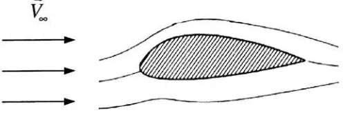
Wind Tunnel Flow 9

Free Air Flow 9

TheCorrectable Interference Transonic Wind Tunnel Concept 14

SchematicDiagramofComputational Grid(upper halfplane_only) 18 Outer

Boundary

ConditionfortheTunnel Calculation 20

Inner(Airfoil

Slit)

Boundary

ConditionoftheTunnelCalculation 20

FlowChartoftheSemi-Automatic Procedure 26

ModelandWall ConfigurationsofAdaptive Wall Test Case 32

Equivalent Inviscid

Body

on Adaptive Wall Test Case 33

Model

Cp

DistributiononAdaptive Wall Test Case 34

Lift CurveonAdaptive Wall Test Case 34

Model andWall ConfigurationonSlotted Wall Test Case 35

EquivalentInviscid

Body

onSlotted Wall Test Case 36

Model

Cp

DistributiononSlotted Wall Test Case 37

Lift CurveonSlotted Wall Test Case 37

Drag

CurveatRe 9,000,000and

C,

0on Original TWNTN4A Grids 41 Lift CurveatRe 9,000,000andM=0.50_on Original TWNTN4A Grids 42

LiftCurveatRe 9,000,000andM 0.65on Original TWNTN4A Grids 43

Lift Curve atRe 9,000,000andM 0.76on Original TWNTN4A Grids 44

Lift CurveatRe=9,000,000andM=0.80_on Original TWNTN4A Grids 45

Drag

CurveatRe 3,000,000and

Q

0onOriginal TWNTN4A Grids 47 Lift CurveatRe 3,000,000andM=_0.50_onOriginal TWNTN4A Grids 48

Lift CurveatRe*3,000,000_andM*0.65 _onOriginal TWNTN4A Grids 49

Lift CurveatRe 3,000,000andM=0.76onOriginal TWNTN4A Grids 50

Lift CurveatRe= _3,000,000_andM*0.80onOriginal TWNTN4A Grids 51

Lift CurveatRe=_9,000,000_andM 0.76onFinerGrids 53

(8)

List

of

Tables

Table Title Page

5.1

Summary

ofGiven Experimental Data Sets 30

5.2

Summary

ofFlow PropertiesontheGiven Data Sets 30

5.3

Summary

ofData Representation Symbols 31

5.4 Swanson/Turkel Shock Wave Table 31

5.5 TWNTN4A ResultonAdaptive Wall TestCase 34

5.6 TWNTN4AResulton Slotted Wall Test Case 37

5.7

Summary

ofFlow Properties onthePart1 39

5.8

Summary

ofFlow PropertiesonthePart 2 39

5.9

Summary

ofFlow Properties onthePart3 39

(9)

List

of

Symbols, Subscripts,

& Abbreviations

Symbols

b Modelspan ortestsection width b/c Model aspect ratio

c Modelchord

Cd

Drag

coefficient

Ci

Liftcoefficient

Cp

Pressurecoefficient

H Tunnel_emptysidewall

boundary

layershapefactorat model location h/c Tunnelhalfheighttochord ratio

k2

Murthy

aspect ratiofactor

M Machnumber

Re Reynoldsnumberbasedon model chord

r Positionvector

S Sidewall

boundary

layercoefficient

V

Velocity

vector

u Componentoftotal_{velocity in}x-direction v Componentoftotal_{velocity in}y-direction w Componentoftotal_{velocity in}z-direction x Stream-wise direction

(longitudinal)

y Verticaldirection

(lateral)

a Angleof attack

3

Compressibility

factor,

Vl-M2

y Ratioof specific heats

r Circulation

8*

Tunnel emptysidewall

boundary

layer displacementthickness Aa Angleof attack correction

AM Machnumbercorrection

A Coefficientoftransonicsmalldisturbanceequation (|> Perturbationpotential

cp Dimensionlessperturbationpotential O Total velocitypotential

(10)

Subscripts

F Freeair

M Model

(airfoil)

R Reference (Tunnel

Reference)

T Tunnel

W Wall

WT Wind Tunnel

oo

Infinity,

far_{away from}a model. Itindicatesthefreeair region

Abbreviations

L.E.

Leading

edge

RMS Root Mean Square

TCT Transonic Cryogenic Tunnel

(11)

Post-Test Implementation

of

(12)

Chapter 1

-

Introduction

Theconditions under which a model is tested in a wind tunnel are not the same as those in

free air. Wind tunnel measured _quantities, e.g. Mach number, Reynolds number, angle of

attack, lift coefficient,

drag

coefficient, moment _coefficient, require corrections to simulate

those that would have been measured in free air condition. In this thesis, the TWNTN4A

codeis usedtocorrect experimental data from theNASA 0.3m Transonic Cryogenic

(Wind)

Tunnel

(TCT)*

tofreeair conditions.

The presence of tunnel walls causes the difference between measurements in a

two-dimensional windtunnel andin free air. Firstofall, tunnel wall presence itself isthe root of

boundary

layer development that doesnot existin free air. Tunnel sidewall

boundary

layers

can interact with shock waves _spanning the test section at transonic speed to induce flow

separation in the model/sidewalljunction region. Airflow in wind tunnels is unlike free air

because tunnel walls influence airflow in the longitudinal and lateral directions in the test

section.Variouseffects are givenbelow:

1. Horizontal buoyancy. It is a variation in static pressure _along theaxis ofthe testsection

resulting from the

thickening

of the

boundary

layeras it progresses toward the exit and

to the resultant effectivereductionofthe flowarea. Itfollowsthat thepressure_{is usually}

progressivelymorenegative as theexit is approached, andthere is hence a

tendency

for

(13)

2. Solid blockage. The presence of a model in the test section reduces the area through

which the air must flow.

Hence,

by

_continuity and Bernoulli'sequation, it increases the

velocity of the air as _{it flows} over the model. It affects all forces and moments

measurements.

3. Wake blockage. Wake behind the model has a mean _{velocity lower} than the tunnel

stream.

According

to thelaw of_continuity,the_velocityoutside thewake must be higher

in order that a constant volume offluid _may pass through the test section. The higher

velocity in the mainstream has a lowered pressure

by

Bernoulli's principle, and this

lowered pressure puts the model in a pressure gradient and results in a _velocity

incrementatthemodel.Itaffects the

drag

measurement.

4. Streamline curvature.Thepresence of_ceilingand floorpreventsthenormal curvature of

theair stream. Themodel appears to havemore camber than _{it actually has. Airfoil in} a

wind tunnel has too much lift and moment about the quarter chord at a given angle of

attack, and

indeed,

theangle of attackis toolargeas well.

It is assumedthat errors due to _{customary failings} of windtunnel noise, tare, angularity of

flow,

local variations in velocity, and temperature fluctuation _{have been already} removed

beforewalleffects are considered.

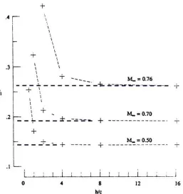
Figure 1.1 illustrates the effect of tunnel half height to chord ratio

(h/c)

versus the lift

coefficient. This quantity h/c is related to some of error factors described above. For

example, the smaller the _quantity

is,

the less area there will be at the test section (solid

blockage)

andthe closer the model andtunnel walls are (streamline curvature). There exists

(14)

number,angle of _attack, andReynolds _number;

however,

thefigure shows the measurement

error of lift coefficient in wind tunnel when the _{quantity h/c} is small. It also shows the

extreme _sensitivityoflift coefficient to the _quantity

h/c,

_particularlyin transonic flow. This

result was measuredforNACA 0012 at 1angle of attack in a

2-D,

straight wall windtunnel

[1].

+

.4 I

.3

\

"*"

--... M>=0.76

+

M-_0.70 +

+

J-_-_ ₊ M_=_0.50

1

J i_J

12 16

h/c

Figure1.1:EffectofTunnel HalfHeighttoChordRatioversusLiftCoefficient

All of above factors affect the data measured in wind tunnels and point to the need for

[image:14.544.137.394.182.455.2]

(15)

Literature Review

Windtunnelwall interferencecorrection_methodologystarted as _earlyas 1931

[2,

3,

4]. Until

the mid 1970s

[5, 6, 7],

wind tunnel data correction utilized a combination of singularities

(e.g.,

source, sink,

doublet,

vortex, etc.) and relied on simple potential flow solutions to

mathematically simulate the flow pattern about an airfoil. Most methods described tunnel

walls as

boundary

_conditions, _using also a collection of these singularities. Theoretical

models determined the form of singularities

imposing

ideal

boundary

conditions.

However,

from themid 1970s

[8, 9],

theformwas determined

by

actual pressure measurements_along

tunnel walls

during

the wind tunnel testing. _{Then using} the linearized potential flow

equations and

boundary

conditions, wall singularities and model singularities are

linearly

superimposed ordecomposedtodeterminetheirrespective strengths.

Along

with the analytical methods to correct wall

interference,

slotted and adaptive wall

transonic test sections are two mechanical developments that can _{significantly} reduce wall

interference compared to straight solid wind tunnel walls. Slotted walls suck out

boundary

layers from tunnel walls so that the horizontal

buoyancy

effects can be reduced. Adaptive

walls can form flow stream configuration on tunnel walls so that it can reduce the stream

curvature effect.

However,

in either_method,other error factorsstill affect thedatameasured

inwindtunnels.

The TWNTN4A computer programcombined the latest analytical andthe mechanical ideas

tocorrect/assesswindtunnel wallinterference. It is a_nonlinear, _transonic, small

disturbance,

(16)

for disturbances caused

by

the side wall

boundary

layer in 2-D wind tunnels. It uses a

nonlinear equationto_accurately model airflow attransonicspeed. Thecodehas asignificant

improvement over classical correction _methods, _particularly for transonic flows.

First,

the

program solves nonlinear equation

including

a higher order term to enhance the transonic

modeling.

Second,

measured data are used in both the exterior and interior

boundary

conditions.

Third,

the program accounts _{approximately for} some influence ofthe sidewall

boundary

layers. Thismethod attemptsto preservethenonlinearinteraction inthetestsection

flow

field,

including

effects of shock waves and

boundary

layers on both the model and

tunnelwalls.

BriefHistoryofTWNTN4A

The TWNTN4A application is an upgraded version of program called TWINTAN

[10]

by

Kemp. The original TWINTAN only accounted for the

top

and bottom wall interference.

Barnwell and Sewall

[11]

improved TWINTAN

by introducing

a simple model of tunnel

sidewall

boundary

layers. This new feature accounted for the additional blockage

interferencecaused

by

thereaction of sidewall

boundary

layerto the model inducedpressure

gradients. This improved program is called TWINTN4

[12],

which is a full four wall

correction scheme.

However,

this new scheme appeared to overcorrect the interference.

Murthy

[13]

explainedtheovercorrection and proposed a modification toit

by involving

the

model aspect ratio in theprogram. The TWINTN4 wasfurther improvedto accountforwall

interferencewithinatunnel

having

flexibly

adapted

top

andbottomwalls. Thisis thecurrent

(17)

In this _thesis, all the results were produced

by

TWNTN4A application, which includes the

(18)

Objective

Theobjective ofthis thesisisto:

1. Understand how the TWNTN4A computer program assesses/corrects the interference

fromwindtunnelwalls.

2.

Develop

a pre- _{and post-processor of} _TWNTN4A

program to save time

by

_replacing

manual operations.

3.

Apply

TWNTN4A program to given experimental datasets and analyze the consequent

results

by

_comparingwithSwanson/Turkel solution, which wastreatedastheinterference

freedata(the reference) becauseoftheabsence offlighttestresults.

4. Provide a new

feature,

variable grid _control, as an option so thatusers have a control of

(19)

Chapter 2

-

TWNTN4A

Theory

Although TWNTN4A is an upgraded version of

TWINTAN,

it is still basedonKemp's ideas

of transonic analysis procedure and correctable interference concept [14]. This procedure

formulatesthe

theory

of

TWNTN4A,

andthen theconceptintroduces thecriterion whenthe

procedure canbeappliedtocorrect wallinterference ina windtunnelattransonic speeds.

Transonic Analysis Procedure

Traditional methods for analysis of wind tunnel wall interference at subsonic speeds are

based on the linear superposition of elemental perturbation potentials _arising from

singularities_representing a model and tunnel walls. At subsonic flow _speed, where thewall

singularities are_clearly distinguishable from those _representing the model, thewall induced

perturbation field can be isolated without ambiguity. At transonic speed,

however,

the

nonlinear interaction among perturbations precludes such a direct definition of the

wall-induced perturbation. A transonic analysis procedure is developed here in principle, which

should yield not _onlya_rationally defined wallinduced perturbationfield but also a criterion

for assessing applicabilityof windtunnel datatoafreeairflightcondition.

Utilizing

theperturbation _velocitypotential concept , thepotential flow ina windtunnelcan

be naturallyexpressedas:

wr=VR-r+twr

(2.1)

*

(20)

Itispresumed that the

boundary

conditions neededtodefinethe windtunnel flow are known

so thata solutionfor

Qm

canbeobtained.Theequation

(2.1)

shows thewindtunnel _velocity

potential is a sum of basic tunnel potential and

(total)

perturbation potential induced

by

tunnel walls andtheairfoil (Figure2.1).

VB

y///////////////////////

^

[image:20.544.142.390.172.276.2]

////////////////////////

Figure 2.1: Wind Tunnel Flow

Now,

utilizingthesame

idea,

afree airflowconditionwithan airfoil can beexpressedas:

F=V-r+

h

(2.2)

In a free air condition, only the presence of airfoil can perturb the

incoming

flow,

which

could be angled to the

leading

edge of _airfoil, because there _{is nothing} to perturb the flow

(Figure 2.2). Theperturbation _<j)M isattributable_entirelyto theairfoil.

[image:20.544.144.392.520.602.2]

(21)

The

boundary

conditions to be imposed on the equation

(2.2)

are the analytic far field

expression forunboundedflowtogetherwith aninner

boundary

conditiondesignedtoassure

that the _resulting perturbation

<j)M

is an appropriate representation ofthe direct influence of

airfoilin a windtunnelflow.

Any

_remainingperturbationinthe tunnelflow is then attributed

to thepresenceoftunnel walls

(<j)w

),

so one_maywrite:

</>w=0m-<PM

(2.3)

Theproposed

boundary

conditiontobe imposedatthemodel and wakeiswritten as:

Iv*J=Iy"aJ

(2-4)

where the brackets denote the

discontinuity

between the upper and lower surfaces of the

model and wake oftheenclosed perturbation _velocityvector. Thestrengths ofthesource and

vortex-like singularities thatare usedtorepresentthe model are assuredtobe identical inthe

wind tunnel and free air flow. As a result of this

boundary

condition, the wall induced

velocity field defined

by

V0W

iscontinuous acrossthemodel and_wake, and_any shock wave

intersecting

the model or wake in the wind tunnel flow will be

identically

located on the

(22)

The basic purpose of wall interference assessment is to examine the _{applicability} of data

measured on the model in a wind tunnel test to free air flight. To this end, it needs to be

asked whether a free air flow exists in which the model shape and surface pressure

distribution areidentical to thosein the tunnel.Askwhetherthe_equality

VF=Vm

(2.5)

can be satisfied everywhere on the model surface.

First,

express the wall induced velocity

fieldasthecombination of even and odd(uniformand_non-uniform)parts:

Vw=V^=V^,s+V^iA

(2.6)

where the subscript S and A represent symmetric and anti-symmetric respectively.

Now,

performing mathematical manipulations:

Equation (2.

1)

=>

Vm

=

V<Pm

=VR+V<t>wr

(2-7)

Equation

(2.2)

=>

VF

=V<D

F =

V

+

V0M

(2.8)

Equation

(2.3)

=> V^. =

V^

+

V^

(2.9)

Substituting

theequation

(2.7)

and

(2.8)

intotheequation(2.5):

?+?*=?*+***

(2-10)

Substitutetheequation

(2.9)

intotheequation(2.10):

(23)

Lastly,

substituting

theequation

(2.6)

intotheequation (2.1

1),

theexpressionbecomes:

K.=V+V^>S+V^

(2.12)

Onecan set

V-=V,+V^iS

(2.13)

ifand_onlyifthesymmetric

(uniformity)

criterion

V<1>w,a=0otVw=Vw<s

(2.14)

is met everywhere onthemodel surface.

Now,

withthecriterion_above, one can _say that theequation

(2.5)

is satisfied everywhere on

themodel surface.

V_F =v_m

(2-5)

Repeated

The free air flow expressed

by

the equation

(2.2)

can now be solved

iteratively

_using the

equation

(2.13)

to update V. After convergence, the wall induced perturbation field is

defined

by

theequation(2.3). Ifthe symmetric

(uniformity)

criterion, equation

(2.14),

is met

within acceptable limits over the model surface, the tunnel data are correctable _simply

by

correctionstoMachnumber andangle of attackderived

by

_expressingtheequation

(2.13)

in

(24)

Correctable Interference

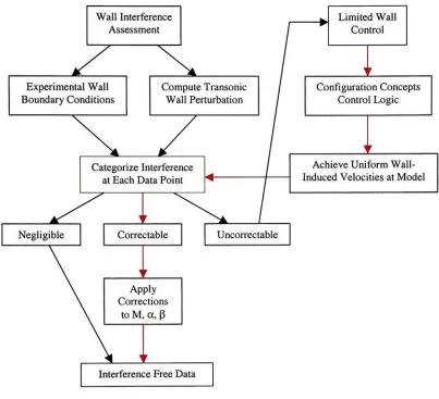
Concept

Kemp's

[14]

correctable interferenceconcept uses the flow chart, Figure 2.3. Aspart ofthis

thesis, the flow chart's red path was assumed to betrue. In other_{words, this} path presumes

that_applying wall control technologies (slotted and/or adaptive _wall) achieves uniform wall

induced velocities at _{the model,} andthen the experimentaldata is categorized as correctable

sothatTWNTN4Acorrection producesthevalidinterference free dataattheend.

This categorization

(negligible,

_correctable, _{uncorrectable)} _is related to the _uniformity

criterion discussed in the _preceding section, the equation (2.14). This thesis checks the

criterion

by

RMS

ACP

value onthe model. When thevalue was close to zero, itcategorized

the data set as negligible and/or correctable (there is no distinction between negligible or

correctable here because TWNTN4A was applied to both cases anyway). When the value

wasnot close to zero,itcategorizedthe dataset as uncorrectable. There is nobordervalueto

evaluate the closeness of zerofor theRMS

ACP

value, butthe table 5.10 (chapter

5)

_clearly

shows the distinction. Please see the end of Chapter 5 for the detailed discussion of this

criterion check.

Satisfaction of the _uniformity criterion was _usually the case

by

_applying the wall control

technologies in this project.

However,

on some _occasions, experimental data fell into the

uncorrectable _category even with the wall control technologies. Since TWNTN4A always

(25)

WallInterference

Assessment

Limited Wall

Control

Experimental Wall

Boundary

Conditions

Negligible

ComputeTransonic

Wall Perturbation

Configuration Concepts

Control Logic

Categorize Interference

atEach Data Point

AchieveUniform

Wall-Induced VelocitiesatModel

Correctable Uncorrectable

Apply Corrections

toM,a,

P

[image:25.544.66.469.67.434.2]

InterferenceFree Data

(26)

Chapter

3

-

Numerical Procedure

TWNTN4A is a _nonlinear, _transonic, small

disturbance,

potential flow program capable of

correcting wall interference effects in 2-D wind tunnels

including

2- and 4-wall correction

capabilityfordisturbancescaused

by

the side wall

boundary

layers.

TWNTN4Aperformsthree calculation cycles - tunnel

calculations, free-aircalculations, and

perturbation flow calculations. In the first cycle, the tunnel calculation employs an inverse

design procedure to determine an _effective, inviscid geometric representation of the test

model, which includes the viscous effects of the model and the interference distortions

imposed

by

thepresence ofthe tunnel walls. Inthe second_{cycle, the}free airflow aboutthis

equivalentinviscid shapeiscomputedto correcttheangle of attack andMachnumber. In the

third cycle, the free air flow is again computed _using the

body

shape obtained in the first

cycle and the corrected free stream condition with modified

boundary

conditions obtained

fromthesecond. The difference betweenthetotalperturbationfromthefirstcycle and model

perturbations obtainedinthethirdare attributableto thewalleffects.

In each calculation cycle, TWNTN4A solves the same _governingequation on thesame grid

with different sets of

boundary

conditions. The

following

describes the _governing _equation,

(27)

Governing

Equation

TWNTN4A solves 2-D small disturbancetransonic potential flow equation. It is a2-D form

of perturbation_velocity potential with airfoilinfree air.Ittakes theform of:

aA^-o₀

:>..2

where:

dx2 dy'

V '

Um

dx

2

Ul

[dx)

(3.1)

(3.2)

Thehigherordertermin is kept in theequation tomodel the transonic flow behavior

{dx)

more accurately. TWNTN4A uses a scaled

(non-dimensionalized)

perturbation potential

definedas:

<p=

UR-c

(3.3)

This dimensionless quantity allows comparisons between solutions with different values of

flow stream velocity.

Substituting

thisrelationinto theequation

(3.1)

and

(3.2)

constructsthe

TWNTN4A governingequation:

A.^?

=₀

dx2 dy2

(3.4)

"

(28)

where:

A=

l-Ml

-(y +

l).M2

.(*-)

U

dx

2 - U

\ ~y

+5

(3.5)

The_quantity

UR

isthe_velocityat

MR

, whereas

U

isthe velocityat

Mm

. Theterm 5 isthe

effect oftheside wall

boundary

layer developed

by

Barnwell andSewall

[11]

andis further

modified

by Murthy

[13]. That is:

where:

S=-2S*

(_

1 2+-MI

H R

(

k2

\

sinh(fc2

)

(3.6)

k2

=

(3.7)

Note that the two-wall correction scheme is constructed if is taken tobe zero since the

side wall term

(5)

_{simply drops}out.

Thetransonic analysis procedureintroduced inchapter2 isupdatedhere because TWNTN4A

utilizesthenon-dimensionalizedperturbation_potential,defined intheequation (3.3).

Equation

(2.1)

Equation

(2.2)

Equation

(2.3)

^_WT _T'

+(pWT

&F

=UT -c

U.

Ut

c

+_<pM

<Pw =<Pwt-<Pm

(3.8)

(3.9)

(29)

Computational

Grid

Figure3.1 shows an example computational grid usedin TWNTN4Aapplication. Thegridis

geometrically stretched forward from the

leading

edge, backward fromthe

trailing

edge, and

vertically in both directions from the slit on which the model

boundary

conditions are

imposed. The geometric _stretching rate in the vertical direction is determined such that an

intermediate gridlinecoincides withthe

top

andbottomtunnel walls. Thissame_{stretching is}

used for calculation of both tunnel and unconstrained free air

flows;

thus the differences

between thesolutionsdue todiscritizationerror are minimized. Themaximum allowable grid

sizeis 100

(longitudinal)

x 100(lateral). A largergrid configuration will be introducedatthe

end ofthischapter.

Lrpper Tunnel Wall

11

[image:29.544.81.466.319.528.2]

Slit

(30)

Three Calculation Cycles with

Boundary

Conditions

1. Tunnel Calculation

The _{tunnel calculation, the} first calculation _cycle, employs an inverse design procedure to

determine an _effective, inviscid geometric representation of _{the test model,} which includes

the viscous effects ofthe model andthe interference distortions imposed

by

thepresence of

the tunnel walls. In _{this cycle,} tunnel and model wall pressure measurements are used as

boundary

conditions on the internal

flow;

the free stream _velocity and Mach number are

specified the same as the experimental testcase. Themeasured pressure data in the form of

pressure coefficient arefirstconvertedto V2

(velocity

_squared)form_usingtheexpression:

^)=1

+ l-|l+

^-M2-C

2 "

N _r

M'

(3.H)

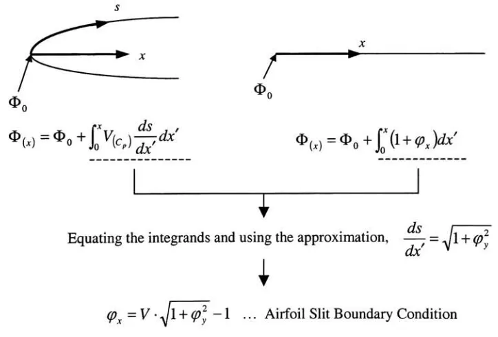
Figure3.2 and3.3 illustratetheouter andinner

boundary

conditions, respectively. The inner

boundary

condition (upperandlowerairfoil _surfaces)istransformedon a slit atthecenterline

(31)

<py

- Given

^=SAy-'

<Px=^V2-<p2y-l

<p=

^<pxAx

+_<plv

<Pyy

=

"A^

[image:31.544.74.484.43.251.2]

<P=

f,Bny'-l+~sgn(y)

Figure 3.2: Outer

Boundary

Condition fortheTunnel Calculation

Note: Wall

boundary

condition,

<px

=

-1,is from V

2 =_u

2

+

v2 =

(l

₊

(px

f

+

<p:

ds . ,

w=o+JX)^7^ dx

r

or

(x)=o+[(l+_<PxW

J

ds

as I

Equating

theintegrandsand_usingthe approximation, - =

Jl

₊

cp

\

dx

q>x

=_V

Jl

₊ (p2

-1 ... AirfoilSlit

Boundary

Condition [image:31.544.102.464.388.633.2]

(32)

Along

with these outer and inner

boundary

_{conditions, there} is an additional

boundary

condition requiredto solvethe tunnel flow calculation. It is theflow direction at thetunnel

upstream

boundary,

the vertical

(upwash)

_velocitycomponent _alongthe forward face ofthe

test section near the upper and lower

bounding

surfaces.

They

are represented

by

SLA

(upper)

& SLB

(lower)

in TWNTN4A code. In practice, these velocity components are

rarely measured, which complicates the correction process

by introducing

a global iteration

todeduce these_velocitycomponents and establishtheproper computational inflow

boundary

condition. TWNTN4A has a _capability of_calculating and _updating the vertical _velocity at

theinflowcorners_using aflowalignment criterion overtheforwardpart oftheairfoil.

Now,

the_governing equation is solved

iteratively

(characteristicsof nonlinear_equation)with

these

boundary

conditions. After the convergence, the resulting small perturbation potential

field constructs the equivalentinviscid

body

(a

body

sensed

by

the tunnel flow

field)

_using

theexpression:

2. Free Air Calculation

In the free air calculation cycle, the inviscid equivalent

body,

determined

by

the tunnel

calculation, is placedin afree air environment at an angle of attack andMach number such

that the lift is identical to that in the tunnel andthe distribution oftotal _velocitymagnitude

(33)

of_attack, known as theKutta condition. Itis represented as a _velocitypotential

jump

in the

perturbation

theory

[18]. The angle of attack is corrected to _satisfy this condition at the

trailing

edge oftheairfoilforthe_{lift corresponding}to the tunnel

flow, i.e.,

a<Pt.e.

=r

(3.13)

During

theconvergenceprocess, the free air

boundary

conditions are

incrementally

changed

in an attempt to minimize the root mean square

(RMS)

difference between the _velocity

distributioncomputedwith thefree air model andthe_{velocity distribution} obtainedfrom the

pressure coefficient data measured with the tunnel model. This requires _updating

Mm

to

minimizeE ,

i.e.,

E2=[VT2-V?}2ds=

j

'P,T

r ^P,F

MTj

ds

(3.14)

This calculation cycle solves the same _governing equation, as mentioned

before,

with outer

andinner

boundary

conditions differentfromthefirstcycle.

Analytically

afar fieldcondition

istheouter

boundary

conditionforthefree air computations. Itmust_satisfythatdisturbances

vanish at the

infinity

(about five chord length above and below from the airfoil surfaces).

Due to computer memory/storage limitations when the original TWINTAN was

developed,

an analytical formoffar field

boundary

condition (still satisfyingthe_vanishingdisturbances

requirementatthe

infinity)

isusedintheprogramand carried ontoTWNTN4A.That is:

r <p=

2n

sgn(z)+tan

(

x~\

^,.

+ y

+1

2_2

aP

x2 +

/32z

(W)

(3.15)

(34)

Klunker

[19]

defines symbols used in theequation

(3.15)

and explains it in details. On the

other

hand,

the inner

boundary

condition offree air cycle is aNeumann condition _using the

values of

<py

extracted

directly

fromthe tunnelflow solution.The

boundary

condition isthen

formed allowing foran angle of attack correction A

[10],

i.e.,

Dl-C-D'2

+

a-(<py

I

-A)

p1

=

y-P^

'

(3.16)

Bl

+C

B2

where the upper and lower signs refer to the airfoil upper and lower surfaces, respectively.

Kemp

[10]

defines symbols used in the equation

(3.16)

and explains it in details. After the

convergence, the correction quantities for angle of attack and Mach number are available

because thelift and

drag

are constrainedtomatchthose ofthetunnel case withthecorrected

angle of attack andMachnumber.

3. Perturbation Calculation

The third calculation cycle is required in order todetermine the classical type wall induced

perturbation _{velocity field. It is} to define that part of the tunnel flow perturbation that is

attributable

directly

to the airfoil. This free air solution about the model is described

by

the

equivalent, inviscid

body

determined

during

the tunnel flow calculation atthecorrectedfree

stream Mach number and angle of attack from the free air calculation. The wall induced

perturbation can betaken asthe difference betweenthe total perturbationobtainedin thefirst

calculation cycle andthemodelinducedperturbation obtainedin thethirdcalculation cycle.

(35)

is the same as in the first cycle (figure 3.3). After the convergence, TWNTN4A uses the

equation

(3.10)

to determine the wall induced perturbation _velocity potential field

by

a

simplesubtraction.

Variable Grid Control

As a new

feature,

variable grid controlhas been introducedtoTWNTN4A application.Atthe

time whenthe originalTWINTAN

[10]

was

developed,

this feature was notincluded in the

program due to the limited computer resources (memory/storage). Even

TWNTN4A,

upgraded version of

TWINTAN,

did not have this _{capability before} this project was

assigned. Thisnewfeaturestill usesthesame geometric _stretchinggridconcept,described in

the previous _section, to represent the flow

field,

but now a user can control the maximum

allowable grid size tomeet thecurrent computational fluiddynamics standardsthat use fine

grids tomodel theflow field.

Oneparameter,

MGS,

definesthe maximum grid sizein the program now.

Ideally

this value

is specified once in the whole program;

however,

it was not possible due to inconsistent

programming methodologies

(mainly

hard-coded multidimensional _array _size) employed

by

several researchers over years of program modifications. It involved considerable effort to

modify

TWNTN4A,

which still requires removals of obsolete _coding and _streamlining the

programflow ingeneral.

Along

withthe parameter, ausermust_specifyafewother variables

(e.g.,

cell

locations,

number of_cells, and cell sizein the input

file)

to generate TWNTN4A

(36)

Chapter 4

- Semi-

Automation

TWNTN4A is an iterative procedure _requiring manual pre- _and

post-processing before and

after each pass (global iteration of TWNTN4A is called pass

1,

pass

2,

and pass

3,

sequentially). Asemi-automatic procedure wasdevelopedas a part ofthisprojecttofacilitate

the _processing of a large number of experimental data files. This procedure _considerably

reducestheTWNTN4Apre- _and

post-processingtime

by

_replacingmanual operations. These

pre- _and

post-processing codes were written in script format that runs underthe

MATLAB*

interpreter (nota standalone executable).

The

following

summarizes the _capability of this procedure. The pre-processing functions

include creating a database out of experimental data files and _{selecting data} sets based on

criteria such as Mach number and Reynolds number. The pre-processor can also

iteratively

update all three passes ofTWNTN4A input files from its own output. The _{post-processing}

functions can store TWNTN4A output to database files for later analysis and can produce a

variety of figures to visualize the results. This semi-automation program produced all the

figuresshowninthis thesis.

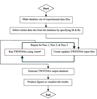
Figure 4. 1 shows a flow chart oftheTWNTN4A correction process performed

by

the semi

automatic procedure. In the

figure,

the

[blue

highlighted

boxes|

represent MATLAB based

(37)

green) is a UNIX script file. Appendix includes an example Auto#

(Auto3)

and all of

MATLAB scriptsforthisprocedure.

<^JStart^>

Make databaseout of experimentaldata files

I

Selectcertaindatasetsfromthedatabase

by

_{specifying M & Re}

1

Repeat for Pass 1,Pass 2,& Pass3

Run TWNTN4A using Auto#

t

11

Create

(update)

TWNTN4Ainput files

1

Generate TWNTN4Aoutputdatabase

Producefigurestovisualizetheresults

[image:37.544.79.478.103.511.2]

End

(38)

SampleRunofSemi-Automatic Procedure

Thissection shows a sample run of semi-automatic procedure withtheactualMATLAB user

interface. Figuresare not numberedbecauseno referenceexistsin this thesis.

Making

databaseoutof experimental data files

Be E* ! web WMow tiff

Do* * 1% (f,' "

| K| ? |Cir.aofy:|cv,ntn4a_yrfle

_*J ,|

l Si EdttfwKwrtt:em*tIMP

Wm _Jfl]*J

ii924pptH 119 E3402pp.tu4 ).J:I il92Spp.tm 119 11928pp.t4 119 il962pp.to4 119 H963.pp.C04 119 l3407pp.CO4 131 ii9e4pp.co4 ii9 Eiseepp.tui us eSllOpptu4 131 jl9ftpptrt 119 E3409pp.to4 134 z3403pp,co4 134 IlM7pJ>.CB4 119 ll963ppt4 119 5l97ppCu4 119 El968pp.to4 119 Z3411pp.cn4 134 y0LJ2pp.EO4 201

run point onrel ft 24 I 0.5036 -4

2 2 0.4971 -4

25 2 0.6020 -4 62 2 0.5007 -4 63 2 0.5989 -4 7 2 0.1983 -4 64 2 0.SSO2 -3 66 2 0.7384 -3 10 2 0.7392 -3

9 3 0.699B -3 3 2 0.694B -3 27 2 0.7O2S -3 65 Z 0.7052 -3 67 2 0.7*03 -3 66 2 0.7B48 -3 11 3 0.7575 -3 32 165 0.S981 -2

05BB 0222 0120 0120 0120 0001 991T 0600 0307 0243 0141 0088 0039 0039 0039 13B4

3026000 _1

2991000 3019000 303 6000 9121000 901,000 8946000 9036000 903SOQQ 9056000 90B7O00 9118000 3014000 30S0O00 9052000 9)01000 912000b 9067000 8900000 . <| Ready

1

Command"mkdb"

makesdatabaseout of

experimentaldata files. PorHthmuPI 1 SJMA

Selecting

certain datasetsfromthe database

by

_{specifying M & Re}

F> Edit iffew Wcfe Wjrrfow tic*?

HBP -IsJjeJ

7ICurrerrl WrwJory:_|CVmtwrtn4alD_y2fle _T]

_J

pickup

BachtReynoldsnumberrange

~3

BachnuBber: 0. 1B50 toD.5150

nuabei: 6550000to94S0000

Command"pickup"selected

certaindatasets.Machnumberis

about0.5andReynoldsnumberis

about9,000,000 inthiscase.A

userhasto_specifytheranges of Machnumber andReynolds

numberinthecode(Seethe Appendix).

.T-.Trrrrr'-w-^i

t>Ed' J> lfwtFormatg>

| tneMM U9t El962pp.tu4 119

E34Q7pp,to4 134

y0813pp.co4 2 OB

y0131pp.tw4 201

E310?pp.i:ii4 134 yQ902pp.tn4 209 y0921ppet4 209 V0131pp.tn4 201

yQ613pp.tt4 20B y0912pp.ts4 2 09

U962pp. tn4 119 El962ppto4 119 yO130pp.to4 201

l3407pp.t4 134

E3407pp.eu4 134

yO902pp.ttrt 209

y092lppto4 209 y0813pp.c4 20B

l3407pp.C<rt 134

hi MafjPfM

HEjoijsj 5007 -4. 49Q3 -4. S004 -2. 4993 -2. 5003 -1. 4994 -1. 4994 -1. 4996 -0. 5005 -0. 49B4 -0 50ZZ -0 5052 -0 .4992 -0 .5014 0 .4998 0 .4993 0 .5009 0 .5006 1 .4995 1 G120 0001 0162 0060 9B57 Z040 03 61 0204 0204 0204 0159 102 0102 0000 0000 0204 0312 9755 9956 trinf 9121000 034 6000 8976000 9965000 9980000 9007000 9979000

902 3000

(39)

Creating

(updating)

TWNTN4A input files

DZSiQHHaaVaM

f*> Ed* v* w* mb Hb

Da:_j .;; t,ft <-I wI

plp2inp Available Nacb. Muabei

? Curat* Olfactory:_|CWriwntn4\2_r _-3J

ami

kD50 k065 n076 L080

Selecta uachnimbetfromChe listabove:076

Ready

"plp2inp"

standsfor "Passl toPass2

input."

Itcreated and updatedthe

TWNTN4AinputfilesforthePass2

from Passl outputfiles

by

_selecting

theMachnumber.

rri

* t *w Favorites loots yelp

tti I | ProaramFie? t-JDnntwtrrta

aC\0_YZF1L

_1)TESTU9 QTEST 134

QTE5T20I

OTE5T20B

QTE5T2D9

GB-Ql_swnturb ! SiOmoso

ttQwoes , pMQ76

QPA5S1

I ffiOM060 !43-C] 3_RE3M

G4_MAT_DB

1_U5_PPLOT Iskfraaspace:31,861

.si _d 5flDATA4C01.DAT GflDATA1C02.DAT M DATA4CQ3.DAT WDATA4C04.DAT a) DATA1C05.DAT >]DATA4C06.DAT MDATA4C07.DAT 0DATA4C08.DAT WDATA4COT.DAT H DATA4C10.DAT MDATA4C11.DAT ]DATA4C12.DAT |W|DATA4C13.0AT W DATA4C14.DAT la]0ATA4CIS.DAT 0DATA1C16.DAT i)DATA4C17.DAT ajDATA4Cie.DAT <J ITvoe J

4 KB OAT Fie 4KB DAT Fie 4KB DAT Fie 4 KB OATFie 4KB DAT Fie 4KB DATHe 4 KB DAT Fie 4KB DAT Fie 4KB DAT FIb 4KB DAT FIb 4KB DATHe 4 KB OATFie 4KB DAT Fie 4KB DATFlc 4 KB DATFie 4KB DAT Re 4KB DATNe 4KB DATFla

etB _|gMyComputer

*l

Running

TWNTN4A_{using Auto3 (Actual}commandis

"auto3".)

JSBIJB

Auto3tasks:

1. Removed_{unnecessary files in}the

currentdirectory.

2. CompiledTWNTN4Aprogram

and executeditonthreedifferent

input files.

3. Kepttheoutputfilesina

Producing

figurestovisualizetheresults

QS?_| St, % W,1 _|_W_|

.Jfll*!

? Curort Bdcry:IC\rmtwrtivlatt_1plol

EplC_lcv

Enter Nacb.nuiibec (n050,*065, etc.):a065

EnterReynoldsnuaber [r9, r3>, etc):r9n

Command"fplt_lcv"

plottedfour lift

curvefigures,theexperimentaldata,

Passl, Pass2,andPass3. Thereare other

commandstoplot model

Cp

distribution,

(41)

Chapter 5

-

Results

The TWNTN4A computer program was applied to all of given experimental data (over 300

data sets). Because most of corrected results showed the same _trend, _only certain cases are

reported here to avoid repetitions of the same type results.

Starting

with a description of [image:41.544.56.498.421.671.2]

givendatasets, thischapter presents anddiscussesresultsfrom theTWNTN4Aprogram.

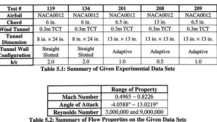
Table 5.1 summarizes the characteristics of given experimental data sets organized

by

test

numbers.Allthe testcases were conducted with NACA0012airfoil at0.3m TCT. Slottedand

adaptive walls are the two differenttunnel wall configurations. Three differentchordlengths

andtwosets oftunneldimensionmake varioustunnel half heighttochord ratios

(h/c),

which

affectthe liftcoefficient _{sensitively (See}the figure 1.1). Table 5.2 shows flow properties of

thedatasets.Datasets cover abroadrange ofMachnumber

including

transonicflow speeds.

Test# 119 134 201 208 209

Airfoil NACA0012 NACA0012 NACA0012 NACA0012 NACA0012

Chord 6 in. 6 in. 6.5 in. 13 in. 6.5 in.

WindTunnel 0.3m TCT 0.3m TCT 0.3m TCT 0.3m TCT 0.3m TCT

Tunnel

Dimension 8 in.x24 in. 8in.x24 in. 13 in.

x 13in. 13in.x 13in. 13 in.x 13 in.

Tunnel Wall

Configuration

Straight

Slotted

Straight

Slotted Adaptive Adaptive Adaptive

h/c 2.0 2.0 1.0 0.5 1.0

Table 5.1:

Summary

ofGivenExperimentalData Sets

Rangeof

Property

Mach Number 0.4965~0.8226

AngleofAttack ~

13.0219

Reynolds Number 3,000,000and9,000,000

(42)

[image:42.544.47.486.370.452.2]

Table 5.3 summarizes the legend (data representation _symbol) used in result figures shown

later. DOT

()

represents theresultfromslotted_wall, whereasASTERISK

(*)

representsthe

result from adaptive wall. The solid black line in result figures represents the comparison

data from Swanson/Turkel [20]. Itis a2-D Navier-Stokes codeto represent the state ofthe

art numerical solution on the airfoil problem. The TWNTN4A results were compared and

validated with this Navier-Stokes numerical solution. Table 5.4 was constructed from

Swanson/Turkel results. It identifies the angle of attack that causes shock wave. This is

included in result figures

by

the verticalblack lines with arrows. It is important to evaluate

TWNTN4A results _concerning shock wave formation. Good results _may not be expected

when shock wave spans windtunnel test section because ofthe interaction with the tunnel

sidewall

boundary

layerstoinduceflowseparationinthemodel/sidewalljunctionregion.

Test Number 119 134 201 208 209

Wall Configuration

Straight

Slotted

Straight

Slotted Adaptive Adaptive Adaptive

H/c 2.0 2.0 1.0 0.5 1.0

Symbol *

Table 5.3:

Summary

ofData RepresentationSymbols

AngleofAttack

0

|

1

|

2

|

3

|

4

|

5 6 7 8

0.50 Y Y

0.65 Y Y

j

|

Y Y Y Y Y

0.76 Y Y Y Y

|

' '

\

Y Y Y Y Y Y Y Y

0.80 Y Y Y Y Y Y Y Y Y Y Y Y Y

Tiible54:Swanson/Tur kelShockV/avelfable

Legend:

(43)

Sample ResultofAdaptiveWall DataSet

This section presents a sample result of_correcting wind tunnel test data from a test section

with adaptive walls. The corrections of adaptive wall data sets _generally showed the same

trend. Thus the current section summarizes most of adaptive wall test cases. To avoid

repetition andto save_{space, this thesis}does notinclude adaptive wall results on_everysingle

data set. The chosen data set has test

#201,

M =

0.7623,

_a =

1.9551,

_andRe = 8,989,000.

Figure 5.1 shows the model and wall configurations. It shows the adaptive wall

characteristic; streamlined tunnel walls to reduce the effect of streamline curvature (see the

chapter 1).

Test

#201,

M=

0.7623,

_a=

1.9551,

_Re=_8,989,000

Figure 5.1: Modeland WallConfigurationsofAdaptiveWall TestCase

TWNTN4A took about 4 seconds to converge on this data set with

170,

1274,

and 283

iterations respectively for thetunnel, free air, andperturbationcalculation cycles. This is the

average computational time anditeration numbers for a single data set on most of adaptive

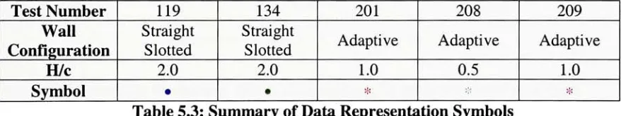
wall testcases. This testcaseusedtheoriginal coarsegrids. Thetunnelcalculation produced

an equivalentinviscid

body

shown inthe figure5.2. Black line represents theoriginal airfoil shape from the wind tunnel _testing, whereas the blue line represents the equivalent inviscid

(44)

other. This indicates the successful convergence of tunnel calculation cycle.

However,

it

raises a question at the

trailing

edge because it is not _closed, which does not _{satisfy Kutta}

condition to have either a stagnation point or a single _velocity at the

trailing

edge. Further

analysis is required on this matter. After the free air calculation cycle, the uniformity

criterion was checked

by

the RMS

Cp

difference (net

difference)

rather than at each single

point on the airfoil. The RMS

ACP

value was 0.017725 that was close to zero compared to

the value of 1.4 ~ 1.8 _on _{non-converged cases.} Thus _the _criterion _was _considered to be

satisfied.

ProgressofEquivalent inviscidBody

[image:44.544.169.369.265.431.2]

0.1 0.2 0.3 0.4 0.5 0.6 0 7 0.8 0.9 1 NormalizedCoordinates,x/c

Figure 5.2: Equivalent Inviscid

Body

onAdaptiveWall TestCase

Distribution ofmodel pressure coefficient is plottedin the figure 5.3. Blue points represent

Cp

distribution from the wind tunnel testing, whereas the TWNTN4A corrected result is

plotted in green. The lower airfoilsurfaceis in an excellent agreement withSwanson/Turkel

(45)

noticeably

inthe liftcurveplot, figure 5.4. The arrowin thefigureindicates thedirection of

theTWNTN4Acorrection.Theright sidedotisthewind_{tunnel test result,}andtheleftoneis

from TWNTN4Acorrection.

Model Pressure CoefficientDistribution LiftCurveof anAdaptive Wall Data Set

0.1 0.2 0.3 0.4 0.5 0.6 0.7 0.8 0.9 1 NormalizedCoordinates,x/c

0 2 4

AngleofAttack,a

Figure5.3:

Model

Cp

Distributionon

AdaptiveWall TestCase

Figure 5.4:

LiftCurveonAdaptiveWallTest Case

Uncorrected Pass 1

Mach Number 0.7623 0.7544

AngleofAttack

[deg.]

1.9551 1.5684

LiftCoefficient 0.3564 0.3612

Drag

Coefficient 0.0203 0.0206 [image:45.544.50.491.161.478.2]

MomentCoefficient -0.0015 -0.0015

[image:45.544.45.505.460.561.2]

(46)

Sample ResultofSlottedWall DataSet

This section is _very similar to the previous section. It presents a sample result on a slotted

wall _{test case,} which can be applied to most of other slotted wall data sets because ofthe

similartrend resultedin theTWNTN4A application. Thechosen datasethas test

#119,

M=

0.7603,

a =

2.0060,

and Re = 9,107,000. _Figure _5.5 _shows _the _model _and wall

configurations onthis testcase. Tunnel walls are straightlines unlikethe adaptivewallcase.

There are plenums on walls toremove the sidewall

boundary

layers (toreduce theeffect of

horizontal buoyancy).

Test

#119,

M=

0.7603,

_a=

2.0060,

Re =9,107,000

Figure5.5: Modeland Wall Configurationon SlottedWall TestCase

The TWNTN4A was _{globally iterated} on slotted wall test cases. One of input

boundary

conditions, SLA and SLB (described in chapter

3),

is always zero on straight tunnel walls.

This permits the global iteration of TWNTN4A program to obtain better results. In this

thesis, theTWNTN4A was _globally applied three times

(Passl, Pass2,

and

Pass3)

on all of

(47)

Here,

the TWNTN4A program took the average of 3 ~ 4 _seconds _{computational} time to

converge on all the passes. Iteration numbers are Passl =

{331, 607,

108},

Pass2 =

{334,

504, 107},

Pass3 =

{336, 402,

106}

for the _{tunnel, free} _air, and perturbation calculation

cycles, respectively. The tunnel calculation computedthese equivalent

body

shapes on each

pass shown in the figure 5.6. Black line represents the original airfoil shape from the

experiment. The blue line is for

Passl,

green is for

Pass2,

and red is for Pass3.

They

are all

veryclose to theactual _shape,which indicatesthesuccessful calculation andconvergenceof

thefirstcycle.

ProgressofEquivalent InviscidBody

0.1 0.2 0.3 0.4 0.5 0.6 0.7 0.8 0.9 1 NormalizedCoordinates,x/c

Figure 5.6: Equivalent Inviscid

Body

onSlotted Wall TestCase

The RMS

Cp

difference was again checked to confirm the satisfaction of the _uniformity

criterion. The firstpasshadtheRMS

ACP

=

0.030192,

_the_secondpasshad

0.029123,

andthe

thirdpassresultedin 0.028297.

They

are close enoughtobezero comparedtonon-converged

cases. Figure 5.7 shows the model

Cp

distribution on this test case. The black line is from

Swanson/Turkel results. The first pass resultis on _{green, the} second is on _red, andthe third

(48)

some agreement to Swanson/Turkel results

(showing

the _superiority of adaptive wall

technology);

however,

it is still in a good agreement to Swanson/Turkel results _considering

the presence of normal shock wave on the upper airfoil surface. Table 5.6 summarizes the

result on this test case.

Again,

the TWNTN4A corrected the angle of attack (about 1

different from the tunnel _measurement) more than other properties. Figure 5.8 shows the

directionofTWNTN4Acorrection on aliftcurve.

-1.5

Model Pressure Coefficient Distribution LiftCurveof aSlotted Wall Data Set

0 0.1 0.2 0.3 0.4 0.5 0.6 0.7 0.8 0.9 NormalizedCoordinates,x/c

Figure5.7:

Model

Cp

Distributionon

SlottedWallTest Case

0.8

0.6 /

0.4

CJ-0.2

y* .

0

1

5

-0.2

-0.4

-0.6

-4 -2 0 2 4 6 8

AngleofAttack,a

Figure 5.8:

IJft CurveonSlottedWall TestCase

Uncorrected Pass 1 Pass2 Pass 3

Mach Number 0.7603 0.7545 0.7492 0.7449

AngleofAttack

[deg.]

2.0060 1.6542 _j 1.2903 0.9116

Lift Coefficient 0.2518 0.2543 0.2566 0.2585

Drag

Coefficient 0.0130 0.0131 0.0132 0.0133

MomentCoefficient 0.0043 0.0043 0.0043 0.0043

[image:48.544.46.496.220.561.2]

(49)

Collectionsof_TWNTN4Aresults (Summary)

The

following

section presents alarge number ofTWNTN4A correction results. The semi

automatic procedure (chapter

4)

was utilizedtoprocessthis largenumberofdatasets. There

are two types of plot used to present_{the results,}

drag

curve andlift curve.

Drag

coefficient

versusMach number curveis usedtodescribeMach number corrections fora given nominal

chord Reynolds number and lift coefficient. Lift coefficient versus angle of attack curve is

used todescribe angle of attack corrections. Verticallines and arrows onlift curves indicate

thepresence of shock wave (SeeTable5.4). Referto table 5.3 forthelegendusedonfigures

presentedhere.

There are three parts in this section. The first part is a collection of results with the

TWNTN4A original grids atRe = 9,000,000. The_{second part} _is _{also with}_the _{original grids}

butatRe =_{3,000,000. The} _third_part_has_{results on}_Re _9,000,000 _with_fine_{grids generated}

by

the variable grid control. Each part flow properties are summarizedin the table

5.7, 5.8,

and5.9. Part 1 and2havethesame nominalMachnumbers:

0.50, 0.65, 0.76,

and0.80.Part 3

is thesame asPart 1 and2 exceptthat the lower Mach number cases (0.50 and

0.65)

are not

shown. Thereason will be discussed inthepart. Shockwave regionisfrom Swanson/Turkel

(50)

Parti

Drag

Curve

MachNumber Reynolds Number LiftCoefficient

Figure 5.9 0.4850~0.8032

8,550,000~9,450,000

[+5%of

9,000,000]

=₀

Lift Curve

Mach Number Reynolds Number ShockWave Region

(a)

Figure 5.10 0.4850-0.5150

[3%of

0.5001

8,550,000~9,450,000

[5%of

9,000,000]

a< &7.0

< a

Figure 5.11 0.6305

~0.6695

[3%of

0.650]

8,550,000~9,450,000

[5%of

9,000,000]

a < &3.0

< a

Figure 5.12 0.7573

~0.7627

[0.35%of

0.760]

8,550,000~9,450,000

[5%of

9,000,000]

a<-1.0&1.0<a

Figure 5.13 0.7968

~0.8032

[0.40%of

0.800]

8,550,000~9,450,000

[5%of

9,000,000]

Any

degree

Part2

LiftCurve

Part3

Lift Curve

Table5.7:

Summary

ofFlow PropertiesonthePart1

Drag

Curve

Mach Number Reynolds Number LiftCoefficient

Figure5.14 0.4850~0.8032

2,850,000-3,150,000

[5%of

3,000,000]

=₀

(a)

Figure 5.15 0.4850-0.5150

[3%of

0.500]

2,850,000-3,150,000

[5%of

3,000,000]

a < &7.0

< a

Figure5.16 0.6305

- 0.6695

[3%of

0.650]

2,850,000-3,150,000

[5%of

3,000,000]

a < &3.0

<a

Figure 5.17 0.7573

- 0.7627

[0.35%of

0.760]

2,850,000-3,150,000

[5%of

3,000,000]

a<-1.0&1.0<a

Figure5.18 0.7968

~0.8032

[0.40%of

0.800]

2,850,000-3,150,000

[5%of

3,000,000]

Any

degree

Table 5.8:

Summary

ofFlow PropertiesonthePart2

(a)

Figure5.19 0.7573

- 0.7627

r0.35%of

0.760]

2,850,000-3,150,000

[image:50.544.52.494.69.536.2]

(51)

Part 1 fRe 9.000.000^

Figure 5.9 shows the

drag

curves on each pass. The uncorrected TWNTN4A data (wind

tunnel measured _quantities) are in reasonable agreement with Swanson/Turkel result. There

is a

tendency

tocollapseintoone point (Rememberthat theremust_{be only}one valid value at

given Mach number, angle of _attack, and Reynolds number) on Mach number ~

0.50;

however,

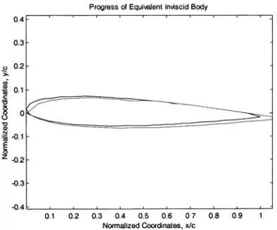
higher Machnumber pointsdonotshow muchimprovementon passtopass.

Figure 5.10 through 5.13 show the lift curves for different Mach numbers. In all

figures,

adaptive wall test cases are _{already in} good agreement with Swanson/Turkel result before

applying theTWNTN4Acorrection. This showsthe _superiorityof adaptive wall technology.

After the first correction, adaptive wall cases did not show much movement on

figures;

however,

most of slotted wall test cases moved toward Swanson/Turkel comparison curve.

After the second correction, slotted wall data sets are in excellent agreement with

Swanson/Turkel results. Liftcurve slopes arealmost identicalto thecomparison curves. Itis

surprisingto see in the figure 5.13 thatTWNTN4A corrects data sets with such high Mach

number(shockwave mustbe_present)at_{moderately high}angle of attack.

It seemed that the third correction was not needed on these cases. The thirdpasses showed

the overcorrection of TWNTN4A program. Notice that high angle of attack cases did not

show _{any improvement} on lower Mach number cases. It is apparent that shock wave was

formed at these high angle of attacks; therefore, it is less

likely

the TWNTN4A program

(52)

Parti

Uncorrected TWNTN4A Data Points TWNTN4ACorrected-_The_{First Pass}

0.65 0.7 0.75 MachNumber,M

TWNTN4A Corrected-_The_{Second Pass} TWNTN4ACorrected

-The Third Pass

[image:52.544.57.483.67.418.2]

(53)

Parti

UncorrectedTWNTN4AData Pomls /*

4-0.8 '

0.6

-U-0.4 _/ l

-I

02

5 o

-0.2

/

"

-0.4 "

TWNTN4A Corrected-The First Pass

0 2 4 6 8 10 12

AngleofAttack,a

2 4

AngleofAttack,a

TWNTN4A Corrected

-The Second Pass

' _\

0.8 '

0.6 /

-""0.4

E a

1 0.2

B

o +/

-0.2

/

-0.4_\_/

TWNTN4A Corrected

-The Third Pass

2 4 6

AngleofAttack,a

1

0.8

0.6

O-0.4

c .9?

I 0.2

s o

-0.2

-0.4

-06

4

*/ *

2 4 6

AngleofAttack,a

[image:53.544.55.476.69.419.2]

(54)

Parti

Uncorrected TWNTN4A Data Points

0.8

0.6 /^

'

0.4 o-I 0.2 o

/ '

S-o,

-0.4

-0.6

-0.8 i

_,

TWNTN4ACorrected

-The First Pass

-2-1012345678 AngleofAttack,a

0.6

/S*

0.4

o-y

I 0.2

1

"-0.2

-0.4

-0.6

-0.8

-3 -2 -1 01 2345678

AngleofAttacka

TWNTN4A Corrected-_{The Second Pass}

0 12 3 4 5 AngleofAttack,a

TWNTN4A Corrected-_{The Third Pass}

0.8

-0.6 .yS

0.4

O-S 0.2 u

-1

-0.2

/ ~

-0.4 '

-0.6 '

[image:54.544.59.481.69.424.2]

-4 -3 -2 -1 0 1 2 3 4 5 AngleofAttack,a

(55)

Parti

0.8

Uncorrected TWNTN4AData Points

0.6 0.4

A

*. O-0.2 / -0.2 . -0.4 ;

/

-0.6 --0.8

-4-3-2 1 0 1 2 3 4 AngleofAttack,a

TWNTN4ACorrected

-TheFirst Pass

0.6

A

* '

' 0.4 */ * U-0.2 * y / . 1 0

&

3-0.2 -0.4 / -0.6

5 6 7 -4-3-2 1 0 12 3 4 5 AngleofAttack,a

0.8

TWNTTN4A Corrected-The Second Pass

0.6 0.4 / . -O-0.2 B

1

%-0.2 0.4

A

-0.6

TWNTN4A Corrected-_{The Third Pass}

0.6 /. ' 0.4 _'/ "-0.2 6 8 -0.2

-04"

/

-0.6

-4-3-2-1012345 AngleofAttack,a

[image:55.544.52.475.67.416.2]

(56)

Parti

Uncorrected TWNTN4A Data Points TWNTN4ACorrected-The First Pass

TWNTN4ACorrected-_The_{Second Pass} TWNTN4ACorrected

-The ThirdPass

10 12 3

[image:56.544.58.471.69.420.2]

AngleofAttack,a

(57)

Part2 (Re 3.000.0001

Drag

curves shownin thefigure 5.14are off

by

0.002

(Cd)

fromthe Swanson/Turkelresults.

Corrected results do not show much

improvement;

rather the correction is in the _wrong

direction. Green and Newman

[21]

obtained the similar results and pointed out that a large

span-wise variation of

Cd

was

detected,

whichTWNTN4Aprogramdoes notaccountfor.

Figure 5.15 through 5.18 show lift curves. There were not enough adaptive wall test cases

available atRe = 3,000,000 from _data_files _supplied

by

NASA. Slotted wall datasets show

improvement from TWNTN4Aon each pass.Thesametype ofdiscussion asthe part 1 holds

here. It takes TWNTN4A correction twice or three times to match with Swanson/Turkel

computational results.

Again,

high angle of attack datacases showed no movement on the

(58)

Part 2

Uncorrected TWNTN4A Data Points TWNTN4A Corrected

-The First Pass

0.55 0.6 0.65 0.7 0.75 0.8

MachNumber,M

0.5 0.55 0.6 0.65 0.7 0.75 0.8 0.6

MachNumber,M

TWNTN4A Corrected

-The Second Pass TWNTN4A Corrected

-TheThird Pass

0.55 0.6 0.65 0.7 0.75 MachNumber,M

[image:58.544.47.470.59.408.2]

).5 0.55 0.6 0.65 0.7 0.75 0.8 0.85 0.9 MachNumber,M

(59)

Part2

UncorrectedTWNTN4A Data Points

0.8

^

: t 0.6 / "-0.4 i i 2 / ' -3 0 -0.2 */ -0.4 -0.6 i

-4-3-2-1 0 1 2 3 4 5 6 7 8 9 10 11 12 AngleofAttack,a

TWNTN4A Corrected

-The First Pass

/ t 0.8 0.6

/

U-0.4 /. e a> 0.2

I

/v 5 o -0.2 -0.4 /

--3 -2 -1 0 1 2 3 4 5 6 7 8 9 10 11 12 AngleofAttack,a

TWNTN4ACorrected-_{The Second Pass}

0.8 0.6 O-0.4 I I 0.2

8

o -0.2 -0.4 -0.6 / _: A ** ' A -4-3-2-101234567

AngleofAttack,a

8 9 10 11 12

TWNTN4A Corrected-