Object search by manipulation

White Rose Research Online URL for this paper:

http://eprints.whiterose.ac.uk/95177/

Version: Accepted Version

Article:

Dogar, MR, Koval, MC, Tallavajhula, A et al. (1 more author) (2014) Object search by

manipulation. Autonomous Robots, 36 (1). pp. 153-167. ISSN 0929-5593

https://doi.org/10.1007/s10514-013-9372-x

[email protected]

https://eprints.whiterose.ac.uk/

Reuse

Unless indicated otherwise, fulltext items are protected by copyright with all rights reserved. The copyright

exception in section 29 of the Copyright, Designs and Patents Act 1988 allows the making of a single copy

solely for the purpose of non-commercial research or private study within the limits of fair dealing. The

publisher or other rights-holder may allow further reproduction and re-use of this version - refer to the White

Rose Research Online record for this item. Where records identify the publisher as the copyright holder,

users can verify any specific terms of use on the publisher’s website.

Takedown

If you consider content in White Rose Research Online to be in breach of UK law, please notify us by

(will be inserted by the editor)

Object Search by Manipulation

Mehmet R. Dogar · Michael C. Koval · Abhijeet Tallavajhula · Siddhartha S. Srinivasa

Received: date / Accepted: date

Abstract We investigate the problem of a robot search-ing for an object. This requires reasonsearch-ing about both perception and manipulation: some objects are moved because the target may be hidden behind them, while others are moved because they block the manipulator’s access to other objects. We contribute a formulation of the object search by manipulation problem using vis-ibility and accessvis-ibility relations between objects. We also propose a greedy algorithm and show that it is optimal under certain conditions. We propose a sec-ond algorithm which takes advantage of the structure of the visibility and accessibility relations between ob-jects to quickly generate plans. Our empirical evalu-ation strongly suggests that our algorithm is optimal under all conditions. We support this claim with a par-tial proof. Finally, we demonstrate an implementation of both algorithms on a real robot using a real object detection system.

1 Introduction

Imagine looking for the salt shaker in a kitchen cabinet. Upon opening the cabinet, you are greeted with a clut-tered view of jars, cans, and boxes—but no salt shaker. It must be hidden near the back of the cabinet, com-pletely obscured by the clutter. You start searching for it by pushing some objects out of the way and moving

Mehmet R. Dogar·Michael C. Koval·Siddhartha S. Srini-vasa

The Robotics Institute, Carnegie Mellon University 5000 Forbes Avenue, Pittsburgh, PA, USA Tel.: +1-412-973-9615

E-mail:{mdogar,mkoval,siddh}@cs.cmu.edu Abhijeet Tallavajhula

Indian Institute of Technology Kharagpur E-mail: [email protected]

others to the counter until, eventually, you reveal your target.

Humans frequently manipulate their environment when searching for objects. If robotic manipulators are to be successful in human environments, they require a similar capability of searching for objects by removing the clutter that is in the way. In this context, clutter removal serves two purposes. First, removing clutter is necessary to gain visibility of the target. Second, it is necessary to gain access to objects that would be oth-erwise inaccessible.

Prior work has addressed the issues of interacting with objects to gain visibility and accessibility as sepa-rate problems. Work on thesensor placement(Espinoza et al 2011) and search by navigation (Ye and Tsotsos 1995,1999;Shubina and Tsotsos 2010;Sjo et al 2009;

Ma et al 2011; Anand et al 2013) problems focuses on moving the sensor to gain visibility. One canoni-cal example of the sensor placement problem is the Art Gallery problem (de Berg et al 2008), which would be equivalent to instrumenting the cabinet with enough sensors to guarantee that the salt shaker is visible. Sim-ilarly, the search by navigation problem would involve moving a mobile sensor through the cabinet to search for the target.

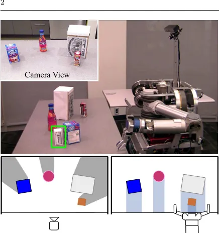
Camera View

Fig. 1 An example of the object search problem on a real robot. The robot is searching for a target object (highlighted by the bounding box) on the table, but its view is occluded (drawn as gray regions) by other objects. The robot must remove these objects to search for the target. Objects may block the robot’s access to other objects.

(Gupta and Sukhatme 2012; Kaelbling and Lozano-Perez 2012) without reference to optimality. One of these works uses a generative model of object-object co-occurrence and spatial constraints (Wong et al 2013) to guide the robot’s search, which is similar to the prior distribution we introduce in §8. Other related work includes exploring the environment with the goal of building three-dimensional models of novel objects using maximally informative actions (van Hoof et al 2012).

One of our key insights is that the object search by manipulation problem requires simultaneously rea-soning about both perception and manipulation. Some objects are moved because they are likely to hide the target, while others are moved only because they pre-vent the manipulator from accessing other objects in the scene.

Fig. 1 shows a scene in which both situations oc-cur. In this figure, HERB (Srinivasa et al 2012)—a robotic platform designed by the Personal Robotics Lab at Carnegie Mellon University—is searching for the white battery pack hidden on a cluttered table. HERB uses its camera to detect and localize objects. As Fig.1-Top shows, HERB is initially unable to detect the battery pack because it is occluded by the blue Pop-Tart box. From HERB’s perspective, the battery pack could be hiding in any of the occluded regions shown in Fig. 1

-Left. With no additional knowledge about the location of the target, HERB must sequentially remove objects from the scene subject to the physical limitations of its manipulator until the target is revealed. For example, Fig. 1-Right shows that HERB is unable to grasp the large white box without first moving the brown juice-box out of the way.

In this paper, we formally describe the object search by manipulation problem by defining theexpected time to find the target as a relevant optimization criterion and the concept ofaccessibility andvisibility relations (§2). Armed with these definitions, we are able to pro-pose and analyze algorithms for object search by ma-nipulation. We make the following theoretical contribu-tions:

Greedy is sometimes optimal:We prove that, under an appropriate definition of utility, the greedy approach to removing objects is optimal under a set of conditions, and provide insight into when it is suboptimal (§3). The connected components algorithm:We intro-duce an alternative algorithm, called theconnected com-ponents algorithm, which takes advantage of the struc-ture of the scene to approach polynomial time com-plexity on some scenes (§5). Our extensive experiments show that this algorithm produces optimal plans under all situations, and we present a partial proof of opti-mality.

Finally, we demonstrate both algorithms on our robot HERB (§6.1 and §6.2) and provide extensive experi-ments that confirm the algorithms’ theoretical proper-ties (§6).

The interplay between visibility and accessibility has revealed deep structure in the object search problem, structure that we were able to identify and exploit to derive the connected components algorithm. We discuss several extensions in§7,§8, and§9. We discuss limita-tions and future work in§10. We believe that our algo-rithms are a step towards enabling robots to perform complex manipulation tasks under high clutter and oc-clusions.

2 Object Search by Manipulation

We start with a scene that is comprised of a known, static world populated with the set of movable objects

with known geometry, but unknown pose. For the re-mainder of this paper, we study a specific variant of the problem in which the target is the only hidden object, i.e.O=Oseen[ {target}. We discuss the presence of other hidden objects in§9.

The robot searches for the target by removing ob-jects fromOseen until the target is revealed to its sen-sors. As objects are removed, fewer objects remain in the scene, which we denote bys✓ Oseen.Oseen refers to the initial set of visible objects and does not change as objects are removed. We define the order in which objects are removed as anarrangement.

Definition 1 (Arrangement) An arrangement of the set of objectsois a bijectionAo:{1, . . . ,|o|} !owhere

Ao(i) is theith_{object removed.}

Additionally, we define Ao(i, j) as the sequence of theith_{through thej}th_{objects removed by arrangement} Ao.

Given an arrangementAo that reveals the target, the expected time to find the target is

E(Ao) =

|o| X

i=1

PAo(i)·TAo(1,i) (1)

wherePAo(i) is the probability that the target will be

revealed after removing objectAo(i) andTAo(1,i)is the

time to move all objects up to and includingAo(i). Our goal is to find the arrangement A⇤

Oseen that

minimizesE(A⇤

Oseen); i.e. reveals the target as quickly

as possible.

2.1 Visibility

When the robot removes a set of objects from the scene it reveals a set of candidate poses of the target object that were previously occluded. Theserevealed configu-rations are defined intarget’s configuration spaceC.

Definition 2 (Revealed Configurations) The set of candidate target poses Co|s ✓ C revealed by re-moving objectso✓s from a scene containing objects

s✓ Oseen.

The probability of revealing the target after remov-ing ofroms is determined by the volume ofCo|s. We

call this therevealed volume of those objects.

Definition 3 (Revealed Volume) The volumeVo|s revealed by removing objects o✓s from a scene con-taining objectss✓ Oseen is

Vo|s=

Z

x2Co|s

P0(x)dx (2)

A

B

C

V

V

V

V

(a) Initial Scene

B

C

V

V

(b)ARemoved

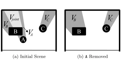
Fig. 2 (a) An example of a scene containing a joint sion. Occlusions are drawn as dark gray and the joint occlu-sions as light gray. (b) The scene afterAis removed.

whereP0(x) is a prior distribution over the pose of the

target object.

We assume thatP0(x) is uniform for the remainder

of this discussion to simplify our examples. We discuss the general case of using a non-uniformP0(x) to encode

semantic knowledge about the scene in§8.

Additionally, we will drop the scenesfrom this no-tation whenever it is obvious from the context. For ex-ample in Fig.2awe writeVAinstead of the more verbose

V{A}|{A,B,C}. Similarly, instead of using VAo(i,j)|Ao(i,|o|)

to refer to the volume revealed between theith_andjth

steps of an arrangement, we will simply useVAo(i,j).

In Fig.2awe show the revealed volumes of objects in an example scene1_.V

joint is jointly occluded by object

AandB, and isnot included in eitherVA orVB. This is becauseVjoint will not be revealed if onlyA or onlyB is removed from the scene.

In Fig.2bwe showVB afterAis removed from the scene in Fig.2a. SinceAis no longer in the scene,VBnow includesVjoint. Similarly, VA would expand to include

VjointifBwas the first object removed from the scene. Regardless of the order in whichAandBare removed, the revealed volume of{A,B}isV{A,B}=VA+VB+Vjoint.

In the most general case, an arbitrary number of objects can jointly occlude a volume. In that case, the volume would be revealed only after all of the occluding objects are removed from the scene.

Given an arrangementAOseenwe compute the

prob-ability that thetargetwill be revealed at theith _step

using the revealed volume

PAOseen(i)=

VAOseen(i)

VOseen

(3)

1 _{We use two-dimensional examples, e.g. Fig.2, throughout}

k

k

A

B

C

V

V

V

A

B

C

V

V

V

(a) Initial Scene

k

k

k

B

C

V

B

V

B

C

V

B

V

(b)ARemoved

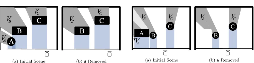
Fig. 3 A scene where the greedy algorithm performs sub-optimally due to an accessibility constraint.

2.2 Accessibility

The manipulator uses a motion planner to grasp an ob-ject and remove it from the scene. To achieve this, the object must beaccessibleto the manipulator. Accessi-bility is blocked by other visible objects, and also by the occluded volume, which the manipulator is forbidden to enter.

Definition 4 (Accessibility Constraint) There is anaccessibility constraint from an objectAto objectB

ifAmust be removed for the manipulator to accessB. Any arrangement of objects in a scene must respect the objects’ accessibility constraints. For example, in Fig. 1-Right, the access to the big box is blocked by the smaller box in front of it.

We identify the accessibility constraints using a mo-tion planner, which returns a manipulator trajectory for each object in the scene. The manipulator trajec-tory for an object sweeps a certain volume in the space (illustrated as light blue regions in Fig.1). Objects that penetrate the swept volume result in accessibility con-straints. Additionally, objects for which the occluded volume penetrates the swept volume also result in ac-cessibility constraints.

We also use the manipulator trajectory for an object

A to computeTA by estimating the time necessary to execute the trajectory on the robot. Since there is only a single action for each object,TAis constant for a given scene and does not depend on the sequence in which objects are removed.

3 Utility and Greedy Search

In this section, we discuss a greedy approach to solving the object search by manipulation problem.

While the overall goal is to minimize the amount of time it takes to find the target, a greedy approach re-quires a utility function to maximize at every step. The faster the robot reveals large volumes, the sooner it will

A

B

C

V

V

V

(a) Initial Scene

C

V

B

V

(b)ARemoved

Fig. 4 A scene where the greedy algorithm performs sub-optimally due to a visibility constraint.

find the target. Using this intuition, we define the util-ity of an object similar to the utilutil-ity measures defined for sensor placement (Ye and Tsotsos 1995; Espinoza et al 2011).

Definition 5 (Utility) Theutility of an objectA is given by

U(A) =VA

TA

This measure naturally lends itself to greedy search. A greedy algorithm for our problem ranks the accessi-ble objects in the scene based on their utility and the removes highest utility object. This results in a new scene, whereby the algorithm repeats until the target is revealed. In the worst case, this continues until all objects are removed.

Unsurprisingly, it is easy to create situations where greedy search is suboptimal. Consider the scene in Fig.3. In this scene,VB&VC> VA. For the sake of simplicity we assume that the time to move each object is similar, henceU(C)> U(A). AsBis not accessible, the greedy al-gorithm comparesU(A) andU(C) and chooses to move

C first, producing the final arrangement C ! A ! B. However, moving the lower utility A first is the opti-mal choice because it reveals VB faster (Fig. 3b), and gives the optimal arrangementA!B!C. It is easy to see that greedy can be made arbitrarily suboptimal by adding more and more objects with utilityU(C) to the scene.

We present a second example of greedy’s subopti-mality in Fig.4. In this scene, all objects are accessible,

The examples in Fig. 3and Fig. 4 may suggest a

k-step lookahead planner for optimality. However, the problem is fundamental: one can create scenes where arbitrarily many objects jointly occlude large volumes, or where arbitrarily many objects block the accessibility to an object that hides a large volume behind it.

Surprisingly, however, it is possible to create non-trivial scenes where greedy search isoptimal. We define the requirements of such scenes in the following theo-rem.

Theorem 1 In a scene where all objects are accessi-ble and no volume is jointly occluded, a planner that is greedy over utility minimizes the expected time to find the target.

Proof Suppose that A⇤ _{is a minimum expected time}

(i.e. optimal) arrangement. For anyi, 1i <|Oseen|, we can create a new arrangement,A, such that theith

and (i+ 1)th_{objects are swapped; i.e.A(i) =A}⇤_{(i+ 1)}

andA(i+ 1) =A⇤_{(i).Amust be a valid arrangement}

because all objects are accessible.

No volume is jointly occluded, so the revealed vol-ume of all objects will stay the same after the swap; i.e.

VA⇤_(i)=V_A(i+1)andV_A⇤_(i+1)=V_A(i). Since the rest of the two arrangements are also identical, using Eq.1and Eq.3, we can compute the difference betweenE(A) and

E(A⇤_{) to be:}

E(A)−E(A⇤_{) =V}

A⇤_(i)·T_A⇤_(i+1)−V_A⇤_(i+1)·T_A⇤_(i). (4)

E(A⇤_{) is optimal, therefore E(A)−E(A}⇤_{) ≥ 0}

and

VA⇤_(i)

TA⇤_(i)

≥VA⇤(i+1) TA⇤_(i+1)

,

which is simplyU(A⇤_(i))≥U(A⇤_{(i+1)). Hence, the}

op-timal arrangement consists of objects sorted in weakly-descending order by their utilities.

There can be more than one weakly-descending or-dering of the objects if multiple objects have the same utility. To see that all weakly-descending orderings are optimal, the same reasoning can be used to show that swapping two objects of the same utility does not change the expected time of an arrangement. ut

This result is rather startling. The greedy algorithm is incredibly efficient in terms of computational com-plexity. At each step, the algorithm finds the accessi-ble object with maximum utility in linear time. In a scene ofnobjects, this results in a total computational complexity of O(n2_{). We show in §5 that the}

worst-case complexity of the optimal search isO(n2₂n_{). The} theorem, however, shows that there are scenes in which greedy is optimal. We shall show in§6that these scenes

do occur surprisingly regularly even with randomly gen-erated object poses. However, as we have shown above, the greedy algorithm can also produce arbitrarily sub-optimal results.

In the next section we present an algorithm based on A-Star search, which is always optimal but has ex-ponential computational complexity. Then, in §5 we present a new algorithm which approaches the polyno-mial complexity of the greedy algorithm, yet maintains optimality in the general case as shown by our empirical evaluations in§6.

4 A-Star Search Algorithm

In this section we present an optimal algorithm for solv-ing the object search by manipulation problem. We first formulate the problem as a deterministic single-source shortest path problem. We then find the optimal solu-tion by executing an A-Star search with an admissible heuristic.

Formulating this problem as a deterministic single-source shortest path problem is possible only because of special structure in the problem. The optimal policy always removes objects from the scene in a determinis-tic order (i.e. an arrangement) until the target is found. See§Afor a derivation of this fact from a formulation of the problem as a Markov decision process.

4.1 Single-Source Shortest Path Problem

Define a directed acyclic graph G = (N, E, c) with nodesN✓2Oseen_{, edgesE✓ O}

seen⇥ Oseen, and cost function c : E !R+_{. A node s 2 N is the set}

visi-ble objects remaining in the scene. The directed edge (s, s\ {a})2Eremoves objectafrom scenes.

Consider the single-source shortest path problem in

GwithOseenas the start node and;as the goal node. Let edges exist between nodessands0_{if they differ by}

a single object and if that object is accessible ins. Ev-ery path from the start to the goal removes all objects from the scene in a different order and corresponds to a different arrangement.

Furthermore, each edge (s, s\ {a})2Ehas cost

c(s, s0_{) =}

✓ _V

a|s

VOseen ◆

TOseen\s0

whereTOseen\s0 is the total time required to reachs 0₌

The sum of the edge costs along any path from the start to the goal is exactly Eq. 1. In other words, the cost of a path in this graph is equal to the expected time to find the target while following corresponding arrangement. Therefore, the minimum-cost inG corre-sponds the optimal arrangementA⇤

Oseenthat minimizes

E(A⇤ Oseen).

4.2 Admissible Heuristic

The single-source shortest path problem can be solved using several well-known algorithms. We use the A-Star search algorithm (Hart et al 1968) with an admissible heuristic to efficiently find the optimal solution. A-Star is optimal if its heuristic is admissible, i.e. does not overestimate the cost from a state to the goal.

Suppose we start at the arbitrary node

s={a1, a2, . . . , an}and the minimum-cost path to the goal is given by the sequence of actions [a1, a2, . . . , an].

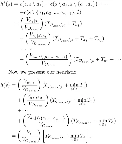
Then, the optimal cost-to-go is

h⇤(s) =c(s, s\a1) +c(s\a1, s\ {a1, a2}) +· · ·

+c(s\ {a1, a2, ..., an−1},;)

=

✓ _V

a1|s

VOseen ◆

(TOseen\s+Ta1)

+

✓ Va2|s\a1

VOseen ◆

(TOseen\s+Ta1+Ta2)

+· · ·

+

✓_V

an|s\{a1,...,an−1}

VOseen ◆

(TOseen\s+Ta1+· · ·+Tan).

Now we present our heuristic,

h(s) =

✓ Va1|s

VOseen ◆

(TOseen\s+ min_a 2sTa)

+

✓ Va2|s\a1

VOseen ◆

(TOseen\s+ min

a2sTa) +· · ·

+

✓_V

an|s\{a1,...,an−1}

VOseen ◆

(TOseen\s+ min_a 2sTa)

=

✓ Vs

VOseen ◆ 

TOseen\s+ min_a 2sTa

& .

Sinceh(s)h⇤_{(s),h(s) is admissible. Intuitively,h(s)}

optimistically reasons that: (1) we execute the minimum-time action and (2) it reveals all of the remaining vol-ume. Since h(s) is admissible, A-Star is optimal and will return the minimum-cost path.

4.3 Computational Complexity

Running an A-Star search on a graph withnnodes and

medges has a worst-case complexity ofO((m+n) logn).

!

B

A

C

D

E

F

Fig. 5 Left: An example scene. Volumes occluded by a single object are shown in dark gray, joint occlusions are shown in light gray, and swept volumes are shown in light blue. Right: The corresponding graph with three connected components.

Algorithm 1: Object Search With Connected Components

1 {c1, c2, ..., cm} FindConnectedComponents 2 foreachconnected component_cido

3 A⇤

ci AStar(ci) 4 A⇤

Oseen [ ] 5 repeat

6 bag ;

7 foreachcomponent arrangementA⇤

ci do 8 forj 1to|ci|do

9 bag.Add(Aci(1, j)) 10 seq arg max

A2bag U(A)

11 Addseqto the end ofA⇤ Oseen 12 Removeseqfrom theA⇤

ci it belongs 13 untilall objects are in the plan 14 returnA⇤

Oseen

Unfortunately, the graph constructed for a scene of size

n=|Oseen|has up to 2nnodes and no more thann2n edges, resulting in a worst-case complexity ofO(n2₂n_). Our experimental results (§6) confirm that A-Star ap-proaches this worst-case bound in practice and it is in-tractable to run this algorithm on large scenes.

5 Connected Components Algorithm

The structure of the object search problem becomes more clear once we represent the visibility and accessi-bility constraints of a scene as a graph. Each node of this graph corresponds to an object in the scene. There is an edge between the nodesAandBif:

– Ais blocking the access toB, or vice versa; or – AandBare jointly occluding a non-zero volume. An example scene and the corresponding graph is in Fig.5.

For example, there are three connected components in Fig.5:{A,B,C},{D}, and{E,F}.

A key insight is that the objects in a connected component do not affect the utility of the objects in another connected component. Hence, we can perform an optimal search, e.g. using A-Star, to solve the ar-rangement problem for a connected component inde-pendently and then merge the solutions to produce a complete arrangement of the scene.

It is non-trivial to merge arrangements of multiple connected components. The complete plan may switch from one connected component to the other and then switch back to a previous component. Our algorithm provides an efficient greedy way to perform this merge. The examples in Fig.3 and Fig. 4 show that the utility of a single object is not informative enough to achieve general optimality with a greedy algorithm. In-stead, we consider the utility of removing multiple ob-jects from the scene.

Definition 6 (Collective Utility)Thecollective util-ity of a set of objectsois given by

U(o) =Vo

To

A general greedy approach which considers the col-lective utility of all possible sequences of all sizes in the scene would quickly become infeasible as the number of such sequences is O(|o|!). In our case, we take ad-vantage of the fact that we have optimal plans for each connected component in which the objects are already sorted. We then need to compute collective utilities of only the prefixes (i.e. the firstkobjects wherekranges from 1 to the size of the connected component) of these optimal sequences.

We present our algorithm in Algorithm1that uses the collective utility of sequences from connected com-ponents to generate an arrangement of the complete scene. It first identifies the connected components in the scene (Line 1). Then it finds the optimal arrange-ment internal to a connected component using A-Star search (Line 3). It then merges these arrangements iter-atively by finding the maximum utility2_{prefixes of the}

optimal arrangements of the connected components. In §6we show that Algorithm1 generates the op-timal result in all scenes we tried it on and it uses a fraction of the time A-Star requires on the complete scene. We present a partial proof of our algorithm’s op-timality in the appendix.

2 _{In the rare event that that multiple sequences share the}

maximum utility, the algorithm breaks the tie by choosing the sequence with the maximum utility prefix recursively.

5.1 Complexity of the Connected Components Algorithm

The connected components algorithm divides the set of objects into smaller sets, runs A-Star on each con-nected component, and then merges the plans for each component. If the scene has no constraints, then there is one object per connected component and this algorithm reduces to the greedy algorithm. Conversely, if the con-straint graph is connected, this algorithm is equivalent to running A-Star on the full scene. Therefore, the per-formance of this algorithm ranges fromO(n2_{), the}

per-formance of the greedy algorithm, toO(n2₂n_{), the}

per-formance of A-Star, depending upon the size of the con-nected components. Geometric limitations put an upper bound on the number of accessibility and joint occlu-sion constraints that are possible in a given scene, so it is unlikely that any scene will exercise the worst case performance. These performance gains will be most sig-nificant on large scenes in which objects are spatially partitioned, e.g. on different shelves in a fridge, but will be modest on small, densely packed scenes.

6 Experiments and Results

We investigated the performance of the different algo-rithms through extensive experiments in simulation and on a real robot. We implemented the greedy, A-Star, and connected components algorithms in OpenRAVE (Diankov and Kuffner 2008). We also implemented a baseline algorithm which randomly picks an accessi-ble object and removes it from the scene. We evalu-ated these algorithms on randomly generevalu-ated scenes. Each scene containednobjects—half juice bottles and half large boxes—that were uniformly distributed over a wide 1.4⇥0.8 m workspace. None of the generated scenes contained hidden objects and the planner used a motion planner based on the capabilities of a sim-ple manipulator. The manipulator was only capable of moving straight, parallel to the table and at a constant speed of 0.1 m/s.

In our implementation, we assume that thetarget

rests stably on the workspace and C = SE(2). We approximate C with a discrete set of configurations

˜

C ⇢ C. Next, we compute a discrete approximation of each set of revealed configurations ˜Co|s={x2C˜:

Ω(x|s\o)^¬Ω(x|s)}using the visibility criterionΩ(x|s) that returns whether x 2 C is visible in the scene s. Finally, we computeVo|sby approximating the integral

overCo|sin Eq.2with a summation over ˜Co|s. In

princi-ple, our framework supports any deterministic visibility criterionΩ:C⇥2Oseen! {_0,1}_{. However partial views}

4 6 8 10 12 Number of Objects

0 5 10 15 20 25 30 35 40 45 E x p ec ted D u ra ti on (s ) A* Components Greedy Random

4 6 8 10 12 Number of Objects

10−2 10−1 100 101 102 103 Planning Time (s)

4 6 8 10 12 Number of Objects 1 2 3 4 5 6 7 8 9 10 11 12 S iz e of L a rg es t C om p on en t 0 25 50 75 100 125 150 175 200 225

Fig. 6 Performance of the random, greedy, A-Star, and connected component planners as a function of number of objects. All results are averaged over approximately 400 random scenes and are plotted with their 95% confidence interval. The planning times are presented in log-scale, where the confidence intervals are also plotted as log-scale relative errors (Baird 1995). The relationship between scene size and the size of the largest connected component is also plotted as a two-dimensional histogram.

4 6 8 10 12

Number of Objects

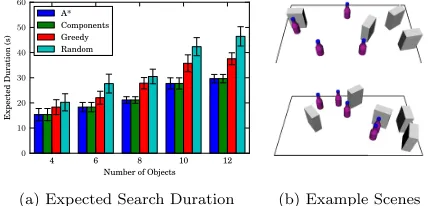
0 10 20 30 40 50 60 E x p ec ted D u ra ti on (s ) A* Components Greedy Random

(a) Expected Search Duration (b) Example Scenes

Fig. 7 (a) 95th_{percentile of expected time to find the target}

(b) Two example scenes where greedy performed poorly. The black lines denote the workspace boundary.

our implementation considers the target at a certain pose visible if and only if it is entirely visible. This is implemented by sampling points on the surface of the target, raytracing from the sensor to each point, and verifying that no rays are occluded.

We present results from scenes with 4, 6, 8, 10, and 12 objects in Fig.6along with the 95% confidence in-tervals. We conducted approximately 400 simulations for each different number of objects, resulting a in to-tal of 2000 different scenes. The data in Fig.6ashows that the greedy algorithm becomes increasingly sub-optimal as the number of objects increases. All three algorithms significantly outperform the random algo-rithm, which serves as a rough upper bound for the ex-pected search duration. Unfortunately, the optimality of A-Star comes with the cost of exponential complex-ity in the number of objects. This complexcomplex-ity causes the planning time of A-Star to dominate the other planning times shown in Fig.6b(note the logarithmic scale).

While still optimal in all 2000 scenes, the connected components algorithm achieves much lower planning times than A-Star. By running A-Star on smaller sub-problems, the connected components algorithm is

expo-nential in the size of the largest connected component,

k, instead of the size of the entire scene. Fig.6cshows that k ⇡n/2 for n  8 and increases when n = 10, causing the large increase in planning time between

n = 8 and n = 10 in Fig. 6b. With fixed computa-tional resources, these results show that the connected components algorithm is capable of solving most scenes of size 2nin the amount of time it would take A-Star to solve a scene of size n. For sparse scenes, the con-nected components algorithm achieves optimality with planning times that are comparable those of the greedy algorithm.

One surprising results of our experiments is that, while greedy is not optimal in the general case, it does remarkably well on average. We found that in 50% of the 2000 different scenes, the greedy algorithm pro-duced the optimal sequence. Our explanation for greedy’s performance is that the geometry of our workspace en-forces a tradeoff between the volume occluded by an object and the number of objects that block its accessi-bility: For an object to occlude a large volume it must be near the front of the workspace, which makes it un-likely that multiple objects can be placed in front of it.

To see the greedy’s worst-case behavior, we plotted the expected time to find the target for the 5% of scenes where greedy performed worst in Fig. 7a. Across all the scenes, the worst performance was 2.04 times the expected duration of the optimal sequence. We show two example scenes where greedy performs poorly in Fig.7b. Both scenes include small bottles blocking ac-cess to large boxes. There is very little volume hidden behind the bottles, so the boxes are—suboptimally— removed late in the plan.

with the extra actions the robot needs to execute due to the greedy algorithm’s suboptimality. In a setting where action executions are fast and greedy is nearly optimal, one should use the greedy algorithm. If action executions are slow and greedy plans are increasingly suboptimal (e.g. in environments with a large number of objects), one should use the connected-components algorithm.

6.1 Real Robot Implementation

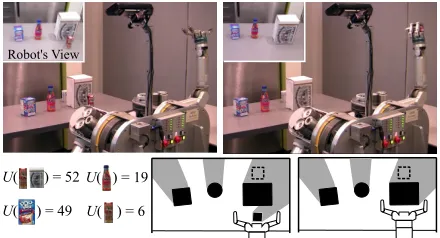
We implemented the greedy and connected components algorithms on our robot HERB. We used HERB’s cam-era and the MOPED (Martinez et al 2010) system to detect and locate objects in the scene. We present an example scene where HERB successfully found the tar-get object using the greedy algorithm in Fig.8. In this scene the target object, a battery pack, is hidden be-hind the large box, which also occludes the largest vol-ume. Since the large box is inaccessible, the greedy planner compares the utilities of the other three ob-jects, and removes the largest utility object at each step. Even though the large box is hiding a large volume, the greedy planner removes it last, resulting in a long task completion time.

In Fig.9the scene is the same but HERB uses the connected components algorithm. There are three con-nected components in this scene{BlueBox},{Bottle}, and{LargeBox,SmallBox}. The connected components algorithm considers the collective utilities of multiple objects from each connected component, including both

U(SmallBox) and U(SmallBox,LargeBox). The utility ofSmallBoxis very small compared with the other im-mediately accessible objects, but combined with the

LargeBox, their utility is large enough that the algo-rithm removesSmallBoxas the first object. It then re-moves the large box and finds the target object. We present the actual footage of these experiments at

http://youtu.be/i06GBj1iDOo.

6.2 Performance in Human Environments

Objects are not distributed randomly in real human en-vironments: they display a structure specific to human clutter. We conducted a simple evaluation of our plan-ner by creating scenes which are similar in structure to human clutter.

For this evaluation we identified three different places where a robot might need to search for an object by manipulation: a bookshelf, a cabinet, and a fridge. We captured images of the natural clutter in these

envi-Table 1 Planning and Execution Times

Total Time Planning Execution Shelf 132.7s 16.1s 116.6s Cabinet 94.6s 26.1s 68.5s Fridge 242.0s 16.7s 225.3

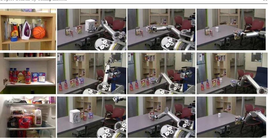
ronments in our lab. We display these images as the leftmost column in Fig.10.

Limitations of our robot’s perception system and the difference between the sizes of a human arm/hand and our robot’s manipulator prevented us from run-ning our planner directly on these scenes. Therefore, we constructed new scenes that are scaled up to the dimensions of HERB’s manipulator and consist of ob-jects that our perception system can reliably detect. We attempted to faithfully mimic the relative size and configuration of objects in the original scenes as much as possible. We hid the target object randomly in the occluded portion of the table.

We present snapshots from our robot’s search for the target as the rows of Fig.10. All plans were auto-matically generated by the connected components al-gorithm and HERB successfully found the target in all three scenes. Tab. 1 shows the planning time, execu-tion time, and the total time it took the robot to find the object. Note that execution time is the dominating factor, emphasizing the importance of generating short plans when searching for objects with a real robot.

7 Planning to Place Objects

The robot must place an object down before picking up another one. If the robot is allowed to place the object at a new pose where it creates new visibility or accessibility relations, then the object search problem becomes a version ofreconfiguration planning which is known to be NP-Hard (Wilfong 1988). We avoid this complexity by placing objects only at poses that do not create new accessibility or visibility relations.

Our formulation requires us to compute the time it takes to manipulate an object before we decide the arrangement. We use fixed placement poses on a nearby empty surface to satisfy this constraint. We found this to be a reasonable strategy in practice: Even when the robot is working in a densely crowded cabinet shelf, there is usually a nearby counter or another shelf to place objects on.

Robot's View

!( ) = 49

!( ) = 19

!( ) = 6

!( ) = 19

!( ) = 6

!( ) = 6 !( ) = 90

Fig. 8 Greedy planner. We present the utility of all accessible objects at each step. The pose of the target (unknown to the robot) is marked with dashed lines in the illustration.

Robot's View

!( ) = 49

!( ) = 19

!( ) = 6

!( ) = 52

Fig. 9 Connected-components planner. The utilities of all prefixes from each connected component are presented at each step.

safely use this volume. In particular, for an arrangement

AOseen, objectAOseen(i) can be placed where:

– it avoids penetratingVAOseen(i+1,|Oseen|),

– it avoids occludingVAOseen(i+1,|Oseen|),

– it avoids blocking access to the objects

AOseen(i+ 1,|Oseen|),

– it avoids colliding the placement poses of the objects

AOseen(1, i−1).

In Fig. 11we illustrate each of these constraints and the remaining feasible placement poses for an object.

Surprisingly, certain scene structures lead to very simple and fixed placement strategies. For example, in a scene where there are no accessibility relations and no joint occlusions (where the greedy algorithm is op-timal), an object can be placed where it was picked up: the robot lifts an object, looks behind it, and places it back. This strategy respects the constraints listed above.

8 Encoding Semantic Knowledge

All of our examples of the object search by manipula-tion problem assume that the target is equally likely

to be found anywhere in the workspace. However, hu-man environments are not random: sehu-mantic knowl-edge about the environment provides useful information about where a hidden object may be found. For exam-ple, a can of soda is more likely to be in the refrigerator than in the dish washer.

There are several existing techniques for learning co-occurrence probabilities objects (Kollar and Roy 2009;

Wong et al 2013) in real environments. We can

natu-rally incorporate this type of semantic knowledge into the prior distributionP0(x). The prior distribution changes

the volume revealed by each target and can be directly exploited by same the greedy, A-Star, and connected components algorithms described above.

For example, suppose that the robot is searching for a bottle of mustard in the refrigerator. Fig.12ashows an example of this scenario where the refrigerator con-tains a small bottle of ketchup K and two large food containersAandB. The mustardMis hidden behind the bottle of ketchup. Assuming that the robot has no prior over the location of the mustard,VA, VB&VK. Assuming

TA =TB =TK, the optimal arrangement with no prior distribution is A ! B ! K because U({A,B}) > U(K) andU(B)> U(K).

However, this plan ignores important semantic knowl-edge about the scene: mustard is more likely to be found near ketchup than the containers of food. This knowl-edge causes P0(x), shown in Fig. 12b, to be peaked

around K. This prior influences the revealed volumes such that VK & VA, VB, the opposite relationship as above. This prior knowledge changes the optimal ar-rangement toK!A!BbecauseU(K)>U({A,B}) and reveals the mustard more quickly.

9 Replanning for Hidden Objects

ob-Fig. 10 Example executions on scenes inspired by real human environments. Scenes are inspired from a cluttered human shelf (top), a cabinet (center), and a fridge (bottom).

Fig. 11 An example illustrating placement contraints. (a) In this scene the small box is moved to the left and then the large box is picked up. Now the planner must place the large box. The large boxcannotbe placed where (b) it will penetrate the volume which is not explored yet; (c) it will occlude the volume which is not explored yet; (d) it will block access to the objects which are not moved yet; (e) it will collide with the new poses of the objects which are already moved. (f) The combined placement constraints for the large box.

K

V

A

B

V

V

(a) Refrigerator Scene (b) Prior DistributionP0(x)

Fig. 12 Example scene where semantic knowledge influences the optimal order of removing objects. The robot is search-ing for the mustard (dotted circle) and has a strong prior distribution that it is near the ketchup (K).

jects in addition to the target. However, objects must be smaller than the target object to avoid the danger of the arm colliding with an hidden object while search-ing for the target. If this condition holds, then one can simply re-execute the planner on the remaining objects whenever an hidden object is revealed. This strategy is

Fig. 13 Example of replanning on a scene with two hidden objects. Each replanning stage is shown as a separate frame along with the corresponding plan. Hidden objects are shown as semi-transparent and the workspace bounds are indicated by a black line.

Fig.13shows an example of replanning on a scene containing six objects. Two objects, shown as semi-transparent in the figure, are initially hidden and are revealed once the occluding objects are removed. The robot begins by executing the connected components planner on a scene containing the four visible objects. After executing the first two actions in that plan, the robot detects that a new object has been revealed and replans for the remaining objects. In this case, the opti-mal ordering is unchanged and the newly-revealed ob-ject is simply appended to the existing plan. After ex-ecuting another action, the second hidden object is re-vealed and the robot must replan a second time. This time, order of the optimal sequence is changed by the addition of the hidden object and it would be subopti-mal to continue executing the previous plan.

10 Future Work

We are excited about exploring this problem deeper and relaxing some of the simplifying assumptions in future work.

Integrated Motion PlanningWe use a motion plan-ner for the manipulator that is conceptually decoupled from finding the optimal arrangement. However, there are aspects of the object search problem that can be integrated into the motion planning process. For exam-ple, there may be multiple trajectories for grasping an object that require differing numbers of objects to be moved out of the way. In this respect, we are excited about studying how a more complex motion planner, e.g. one returning a minimum-constraint violation tra-jectory (Hauser 2012), can be integrated into our sys-tem. The object search formulation can also take into account the motion of moving from one object to the next one, trying to minimize the time spent in between. This can make the object search problem similar to the

traveling agent problem (Moizumi and Cybenko 2001) where the latencies between nodes produced are pro-duced by a motion planner.

Improved Perception Model.Our framework allows for any sensor model. We will explore relaxing the con-servative requirement of the entire target being visible to other perceptual models that address partial visibil-ity.

Integrated Sensor Planning. Aside from reaching to objects, the robot does not move its base in our cur-rent implementation. Through combining the ability of search by manipulation with sensor planning, the robot can find targets faster. Sensor planning would include working with multiple camera poses and planning for the base when searching for a target in a larger envi-ronment.

{A,B,C} B A

C

{B,C}

{A,C}

{A,B} ... ...

A

C ...

...

found

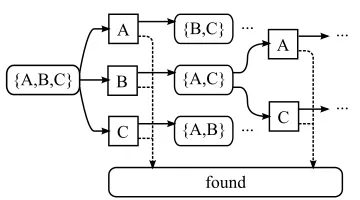
Fig. 14 Transition graph of the of the object search MDP. States (rounded rectangles) are sets of visible objects and actions (squares) correspond to removing an object from the scene. Each action has a probability of revealingtargetand transitioning intofound.

A Formulation as a Markov Decision Process

In this section, we formulate the object search problem as a Markov decision process (MDP) and show that the opti-mal policy minimizes the expected time to find the target. Next, we show that the MDP is deterministic and that each policy corresponds to an arrangement. This provides insight into how the A-Star search algorithm can be used to find the optimal policy for a stochastic problem.

A MDP is the four-tuple (S, A, Γ, R) whereSis the state space,Ais the action space,Γ(s0_{|s, a) is the transition model,} andR(s, a) is the reward function (Kaelbling et al 1996).

For the object search problem, the state s 2 2Oseen_[

{found}is the set of visible objects remaining in the scene and an absorbing goal state foundthat corresponds to the target being visible. The scene starts with all objects present s0=Oseenand the robot sequentially chooses an objecta2 sto remove. After removinga, we transition to the successor states0_{according to}

Γ(s0_{|s, a) =}

(

1−Va|s

Vs :s

0_{=s\ {a}} Va|s

Vs :s

0_=found

and receive reward R(s, a) = −Ta. This process continues until there is a transition intofoundand the MDP terminates with zero reward. Fig.14shows a graphical depiction of the state transition graph for a scene with three objects{A,B,C}

and no accessibility relations.

A policyπ: S !Aspecifies which action π(s) to take when in states. In the case of the object search problem,π dictates which object to remove from the scene at each step. We wish to find the optimal policyπ⇤ _{that maximizes the} sum of expected future rewardE[P|Oseen|

t=1 R(st, at)]. Any policyπ induces the value function Λπ _{: S !}

R, whereΛπ_{(s) is the sum of expected future reward from} start-ing in state sand following π to termination.3 _{The value}

function of the optimal policyπ⇤_{satisfies the Bellman} equa-tion

Λπ⇤(s) = max a2A

X

s0_2S

Γ(s0_{|s, a)}h

R(s, a) +Λπ⇤(s0₎i

, (5)

which recursively relates the value of stateswith that of its successors (Kaelbling et al 1996).

We can take advantage of the structure of the object search problem to reduce the Bellman equation to a simpler

form. First, the object search problem has a sparse transi-tion model:Γ(s0_{|s, a) = 0 for alls}0_{62 {s\a,found}. Second,} Λπ

(found) = 0 for the absorbing goal state. Using these ob-servations, we can simplify Eq.5to

Λπ⇤(s) = max a2s

h

R(s, a) +Γ(s\ {a}|s, a)Λπ⇤

(s\ {a}) +Γ(found|s, a)Λπ⇤

(found)i = max

a2s



−Ta+

✓

1−Va|s

Vs

◆

Λπ⇤

(s\ {a})

)

,

which, surprisingly, has the same form as the value function of a deterministic MDP. This agrees with our earlier intuition: while the outcome the object search problem is stochastic, the optimal order of removing objects is completely deterministic.

In fact,π is equivalent to an arrangement Aπ Oseen that

specifies an open-loop order in which to remove objects. Dur-ing execution objects are removed accordDur-ing toAπ

Oseen until

the target is revealed and the robot halts (i.e. transitions to

found). This equivalence is what enables us to formulate the object search problem as a deterministic search in§4.

B Optimality of Connected Components

We present a partial proof of optimality for Algorithm1. We state a property of the collective utility as a lemma.

Lemma 1 Given an arrangementAo, U(Ao(1,|o|))≥U(Ao(1, k)) =) U(Ao(k+ 1,|o|))≥U(Ao(1,|o|))

In other words, if the utility of the complete arrangement is larger than the utility of the firstkobjects, then the utility of the last|o| −k objects must be larger than the utility of the complete arrangement.

Proof We are given that

VAo(1,k)+VAo(k+1,|o|)

TAo(1,k)+TAo(k+1,|o|)

≥VAo(1,k)

TAo(1,k)

Rearranging yields

VAo(k+1,|o|)·TAo(1,k)≥VAo(1,k)·TAo(k+1,|o|)

Adding VAo(k+1,|o|)·TAo(k+1,|o|) to both sides and

rear-ranging, we get VAo(k+1,|o|)

TAo(k+1,|o|)

≥VAo(1,k)+VAo(k+1,|o|)

TAo(1,k)+TAo(k+1,|o|)

u t

Theorem 2 Given an optimal arrangement of a sceneA⇤_,

for any two adjacent sequence of objects in the arrangement

A⇤_{(i, j)andA}⇤_{(j+ 1, k), whereij < k, if there are}

nei-ther accessibility constraints nor joint occlusions between the objects in the two sequences (i.e. if the sequences are from different connected components), then the utility of the for-mer sequence is greater than or equal to the utility of the latter sequence:U(A⇤_{(i, j))≥U(A}⇤_{(j+ 1, k)).}

Proof The proof proceeds similar to the proof of Theorem1. We create a new arrangementAthat is identical to A⇤ ex-cept that the two adjacent sequences are swapped:

A(i, i+k−j) =A⇤_{(j+ 1, k) and}

A(i+k−j+ 1, k) =A⇤_{(i, j).Amust be a valid arrangement} since we are given that no object inA⇤_{(i, j) is blocking} ac-cess to A⇤_{(j+ 1, k). Then we can compute the difference} E(A)−E(A⇤_{) to be:}

j

X

l=i

✓_V

A⇤₍l)

VOseen

·TA⇤₍j+1,k)

◆

−

k

X

l=j+1

✓_V

A⇤₍l)

VOseen

·TA⇤₍i,j)

◆

SinceA⇤_{is optimal,E(A)−E(A}⇤_{)≥0. After canceling} out the common terms and rearranging, we are left with

j

P

l=i VA⇤₍l)

TA⇤₍i,j)

≥

k

P

l=j+1

VA⇤(l)

TA⇤₍j+1,k)

Simply,U(A⇤_{(i, j))≥U(A}⇤_{(j+ 1, k)). ut} We state a lemma and leave its proof to future work.

Lemma 2 The relative ordering of objects in the optimal arrangement of a connected component will be preserved in the optimal ordering for the complete scene. Formally, ifA⇤ c

is the optimal arrangement for a connected componentc, and

A⇤

ois the optimal arrangement ofo, such thatc✓o, then i < j =) A⇤−1

o (A⇤c(i))<A⇤−o 1(A⇤c(j))

where1i, j |c|, andA⇤−1

o returns the index of an object

in the arrangementA⇤ o.

Finally we can prove that the connected components al-gorithm is optimal.

Theorem 3 Let’s say we are givenmconnected components of a set of objects,o, and we are also given an optimal ar-rangement for each connected componentAcifori= 1, . . . , m.

Let’s say we computed the utility of all sequences of objects in the formAci(1, j)for alli= 1, . . . , mandj= 1, . . . ,|ci|,

and foundAc⇤(1, j⇤)to have the maximum utility. Then an

optimal arrangement forostarts withAc⇤(1, j⇤).

Proof Assume that the optimal arrangement A⇤

o does not start withAc⇤(1, j⇤). We will prove that this is not possible.

Given an arrangement ofo, we can view it as a series of partitions, where each partition consists of a contiguous sequence of objects from the same connected component. Due to Lemma2, each such partition inA⇤

o can be represented as subsequences of the connected component arrangements

Aci. In particular, we are interested in two partitions of the

optimal arrangement ofo:

A⇤

o= [Ac0(1, j0). . .Ac⇤(k, l). . .]

wherec0_{is one of the connected components, and 1j}0_{ |c}0_|.

Ac⇤(k, l) is the partition that includes the objectAc⇤(j⇤),

hencekj⇤_{l. We know thatA}

c⇤(1, j⇤) has the maximum

utility of all the sequences in the formAci(1, j) whereci is

any connected component andj= 1, . . . ,|ci_{|. Then,} U(Ac⇤(1, j⇤))> U(Ac⇤(1, k−1)) (6)

and also

Using Lemma1and Eq.6, we get U(Ac⇤(k, j⇤))> U(Ac⇤(1, j⇤))

Then from Eq.7,

U(Ac⇤(k, j⇤))_{> U}(A_c0(1, j0)) (8)

Considering the utilities of all the partitions inA⇤ oup to

Ac⇤(k, l), we know that they should be ordered in descreasing

order of utility and be larger thanAc⇤(k, j⇤) (Theorem2):

U(Ac0(1, j0))> ... > U(Ac⇤(k, j⇤))

which contradicts Eq.8. ut Acknowledgements Special thanks to the members of the Personal Robotics Lab at Carnegie Mellon University for in-sightful comments and discussions. This material is based upon work supported by NSF-IIS-0916557 and NSF-EEC-0540865.

References

Anand A, Koppula HS, Joachims T, Saxena A (2013) Contextually guided semantic labeling and search for three-dimensional point clouds. International Journal of Robotics Research 32(1):19–34

Baird D (1995) Experimentation: An introduction to mea-surement theory and experiment design. Prentice-Hall (Englewood Cliffs, NJ)

Ben-Shahar O, Rivlin E (1998) Practical pushing planning for rearrangement tasks. IEEE Transactions on Robotics and Automation 14:549–565

van den Berg JP, Stilman M, Kuffner J, Lin MC, Manocha D (2008) Path planning among movable obstacles: A proba-bilistically complete approach. In: In International Work-shop on the Algorithmic Foundations of Robotics, pp 599– 614

de Berg M, Cheong O, van Kreveld M, Overmars M (2008) Computational Geometry: Algorithms and Applications. Springer

Chen P, Hwang Y (1991) Practical path planning among movable obstacles. In: IEEE International Conference on Robotics and Automation

Diankov R, Kuffner J (2008) OpenRAVE: A Planning Archi-tecture for Autonomous Robotics. Tech. Rep. CMU-RI-TR-08-34, Robotics Institute

Dogar M, Srinivasa S (2012) A planning framework for non-prehensile manipulation under clutter and uncertainty. Autonomous Robots 33(3):217–236

Espinoza J, Sarmiento A, Murrieta-Cid R, Hutchinson S (2011) Motion Planning Strategy for Finding an Object with a Mobile Manipulator in Three-Dimensional Envi-ronments. Advanced Robotics

Gupta M, Sukhatme G (2012) Interactive perception in clut-ter. In: The RSS 2012 Workshop on Robots in Clutter: Manipulation, Perception and Navigation in Human En-vironments

Hart PE, Nilsson NJ, Raphael B (1968) A formal basis for the heuristic determination of minimum cost paths. IEEE Transactions On Systems Science And Cybernetics 4(2):100–107

Hauser K (2012) The minimum constraint removal problem with three robotics applications. In: Workshop on the Al-gorithmic Foundations of Robotics (WAFR)

van Hoof H, Kroemer O, Ben Amor H, Peters J (2012) Max-imally informative interaction learning for scene explo-ration. In: IEEE/RSJ International Conference on Intel-ligent Robots and Systems, IEEE, pp 5152–5158 Hopcroft J, Tarjan R (1973) Algorithm 447: efficient

algo-rithms for graph manipulation. Communications of the ACM 16(6)

Kaelbling L, Lozano-Perez T (2012) Unifying perception, es-timation and action for mobile manipulation via belief space planning. In: IEEE International Conference on Robotics and Automation

Kaelbling LP, Littman ML, Moore AW (1996) Reinforcement learning: A survey. Journal of Artificial Intelligence Re-search

Kollar T, Roy N (2009) Utilizing object and object-scene context when planning to find things. In: IEEE In-ternational Conference on Robotics and Automation Ma J, Chung TH, Burdick J (2011) A probabilistic framework

for object search with 6-dof pose estimation. International Journal of Robotics Research 30(10):1209–1228 Martinez M, Collet A, Srinivasa S (2010) MOPED: A

Scal-able and Low Latency Object Recognition and Pose Es-timation System. In: IEEE International Conference on Robotics and Automation

Moizumi K, Cybenko G (2001) The traveling agent problem. Mathematics of Control, Signals, and Systems (MCSS) 14(3):213–232

Ota J (2009) Rearrangement planning of multiple movable objects by a mobile robot. Advanced Robotics pp 1–18 Overmars MH, Nieuwenhuisen D, Nieuwenhuisen D, Frank

A, Overmars H (2006) An effective framework for path planning amidst movable obstacles. In: In International Workshop on the Algorithmic Foundations of Robotics Shubina K, Tsotsos J (2010) Visual search for an object in a

3d environment using a mobile robot. Computer Vision and Image Understanding pp 535–547

Sjo K, Lopez D, Paul C, Jensfelt P, Kragic D (2009) Object search and localization for an indoor mobile robot. Jour-nal of Computing and Information Technology pp 67–80 Srinivasa S, Berenson D, Cakmak M, Collet Romea A, Dogar M, Dragan A, Knepper RA, Niemueller TD, Strabala K, Vandeweghe JM, Ziegler J (2012) Herb 2.0: Lessons learned from developing a mobile manipulator for the home. Proceedings of the IEEE 100(8):1–19

Stilman M, Schamburek JU, Kuffner J, Asfour T (2007) Ma-nipulation planning among movable obstacles. In: IEEE International Conference on Robotics and Automation Wilfong G (1988) Motion planning in the presence of movable

obstacles. In: Proceedings of the Fourth Annual Sympo-sium on Computational Geometry, pp 279–288

Wong LL, Kaelbling LP, Lozano-P´erez T (2013) Manipulation-based active search for occluded ob-jects. In: IEEE International Conference on Robotics and Automation

Ye Y, Tsotsos J (1995) Where to look next in 3d object search. In: IEEE International Symposium on Computer Vision Ye Y, Tsotsos J (1999) Sensor planning for 3d object search.