Improved methodology for the automated classification of periodic variable stars

Improved methodology for the automated classification of periodic

variable stars

J. Blomme,

L. M. Sarro,

F. T. O’Donovan,

J. Debosscher,

T. Brown,

M. Lopez,

P. Dubath,

L. Rimoldini,

D. Charbonneau,

E. Dunham,

G. Mandushev,

D. R. Ciardi,

J. De Ridder

and C. Aerts

1_{Instituut voor Sterrenkunde, Katholieke Universiteit Leuven, Celestijnenlaan 200D, B-3001 Leuven, Belgium} 2_{Dpt. de Inteligencia Artificial, UNED, Juan del Rosal, 16, 28040 Madrid, Spain}

3_{California Institute of Technology, 1200 E. California Blvd. Pasadena, CA 91125, USA} 4_{Las Cumbres Observatory Global Telescope, Goleta, CA 93117, USA}

5_{Department of Physics, University of California, Santa Barbara, CA 93106, USA}

6_{Departamento de Astrof´ısica, Centro de Astrobiolog´ıa (INTA-CSIC), PO Box 78, E-28691 Villanueva de la Ca˜nada, Spain} 7_{Geneva Observatory, Chemin d’ ´Ecogia 16, CH-1290 Versoix, Switzerland}

8_{Harvard–Smithsonian Center for Astrophysics, 60 Garden Street, MA 02138, USA} 9_{Lowell Observatory, 1400 W. Mars Hill Road, Flagstaff, AZ 86001, USA} 10_{NASA Exoplanet Science Institute/Caltech, Pasadena, CA 91125, USA}

11_{Department of Astrophysics, IMAPP, Radboud University Nijmegen, PO Box 9010, 6500 GL Nijmegem, the Netherlands}

Accepted 2011 July 18. Received 2011 July 18; in original form 2010 October 2

A B S T R A C T

We present a novel automated methodology to detect and classify periodic variable stars in a large data base of photometric time series. The methods are based on multivariate Bayesian statistics and use a multistage approach. We applied our method to the ground-based data of the Trans-Atlantic Exoplanet Survey (TrES) Lyr1 field, which is also observed by theKepler

satellite, covering∼26 000 stars. We found many eclipsing binaries as well as classical non-radial pulsators, such as slowly pulsating B stars,γDoradus,βCephei andδScuti stars. Also a few classical radial pulsators were found.

Key words: methods: data analysis – methods: statistical – techniques: photometric.

1 I N T R O D U C T I O N

In recent years there has been a rapid progress in astronomical in-strumentation giving us an enormous amount of new time-resolved photometric data, resulting in large data bases. These data bases contain many light curves of variable stars, both of known and unknown nature. Well-known examples are the large data bases re-sulting from theCoRoT(Fridlund et al. 2006) andKepler(Gilliland et al. 2010) space missions, containing respectively∼100 000 and

∼150 000 light curves so far. The ESAGaiamission, expected to be launched in 2012, will monitor about one billion stars during five years. Besides the space missions, also large-scale photometric monitoring of stars with ground-based automated telescopes de-liver large numbers of light curves. The challenging task of a fast and automated detection and classification of new variable stars is therefore a necessary first step in order to make them available for further research and to study their group properties.

Several efforts have already been made to detect and classify variable stars. In the framework of the CoRoT mission, a

_{E-mail: [email protected]}

cedure for fast light-curve analysis and derivation of classifica-tion parameters was developed by Debosscher et al. (2007). That algorithm searches for a fixed number of frequencies and over-tones, giving the same set of parameters for each star. The variable stars were then classified using a Gaussian classifier (Debosscher et al. 2007, 2009) and a Bayesian network classifier (Sarro et al. 2009).

In this paper, we present a new version of this method to detect and classify periodic variable stars. In contrast to the previous versions, the new automated methodology only uses significant frequencies and overtones to classify the variables with it giving rise to less con-fusion, especially when dealing with ground-based data. In order to be able to deal with a variable number of parameters, we also in-troduce a novel multistage approach. This new methodology offers much more flexibility. We applied this method to the ground-based photometric data of the Trans-Atlantic Exoplanet Survey (TrES) Lyr1 field, covering about∼26 000 stars. The classification algo-rithm considers various classes of non-radial pulsators, such as

2 A N E W M E T H O D O L O G Y

2.1 Variability detection

To detect and extract the variables we performed an automated frequency analysis on all time series. The algorithm first checks for a possible polynomial trend up to order 2 and subtracts it, as it can have a large detrimental influence on the frequency spectrum through aliasing. The order of the trend was determined using a classical likelihood-ratio test. Although the coefficients of the trend are recomputed each time a new oscillation frequency is added to the fit, the order of the trend remains fixed.

After detrending, the algorithm searches for significant frequen-cies and overtones in the residuals, using Fourier analysis. The algorithm searches for the frequency with the highest amplitude in the discrete Fourier transform and checks if this period is signif-icant, using the false alarm probability (Horne & Baliunas 1986; Schwarzenberg-Czerny 1998). Note that a detected frequency peak can be significant but unreliable. Reliability is checked through pre-specified frequency intervals that are not trustworthy (e.g. around multiples of 1 c/d for ground-based data). Unreliable frequencies are pre-whitened, but flagged as ‘unreliable’ and are not used for classification. If the frequency is the first significant reliable fre-quency, then the algorithm checks whether half of this frequency is also significant and reliable. In this case, the original new frequency is replaced with half of this frequency to better model the binary light curves. In a next step, the algorithm searches for significant overtones, using the likelihood-ratio test, to model possible non-sinusoidal variations (like those of RR Lyr stars). This procedure is repeated as long as significant frequencies are found. These fre-quenciesνn can be used to make a harmonic best fit to the light curve of the form

f(t)= K

i=0

ai(t−t0)i

+

N

n=0

M

m=1

bn,msin (2πνnm(t−t0))

+cn,mcos (2πνnm(t−t0)), (1)

with 0≤K≤2 the order of the trend, andN, the number of signif-icant frequencies, determined using the false alarm probability and M≥1, the number of harmonics, determined using the likelihood-ratio test.

The frequency analysis method used by Debosscher et al. (2007) performs well on properly reduced satellite data for which it was designed, but not on noisier ground-based data, as many insignifi-cant frequencies and overtones can degrade the performance of the classifier.

2.2 The classifier

The aim of supervised classification is to assign to each variable target a probability that it belongs to a particular pre-defined vari-ability class, given a set of observed parameters. This set of parame-ters (also called attributes) is obtained from the variability detection pipeline described above and contains frequencies, amplitudes and phase differences. The classifier relies on a set of known examples, the so-called training set, of each class that needs to represent well the entire variability class.

We used a novel multistage approach, where the classification problem is divided into several sequential steps. This classifier

par-titions the set of given variability classesCi, into two or more parts: C(1)_{, C}(2)_,

. . .. This simplifies the classification by degrading the level of detail to a smaller number of categories. Each of these partitionsC(i)_{, which can contain several variability classes, is then}

again splitted intoC(i,1)_,C(i,2)_{,. . ., which in turn can be partitioned}

intoC(i,j ,1)_,C(i,j ,2)_{, and so on, each time specializing the}

classifi-cation until each subpartition contains only one variability class. These partitions can be represented in a tree.

This approach offers several advantages compared to a single-stage classifier. The main advantage of this approach is that in each stage a different classifier and a different set of attributes can be used. This is important as attributes carrying useful information for the separation of two classes can be useless or even harmful for dis-tinguishing other classes. In each stage, informationless attributes for the separation of the classes of interest can be removed, thereby significantly reducing possible confusion. In addition, it is also pos-sible to have a variable number of attributes. This allows us to make different branches for mono- versus multi-periodic pulsators. In this way we do not need a fixed set of attributes, thereby avoiding the introduction of spurious frequencies or overtones, which was sometimes the case in Debosscher et al. (2007). As already men-tioned, this too is important as insignificant attributes can degrade the performance of the classifier.

We took each of the classifier nodes in the multistage tree as a Gaussian mixture classifier. The Gaussian mixture classifier is based on the general law of Bayes:

P(C=ci|A=a)=

L(A=a|C=ci)P(C=ci)

Nc

i=1L(A=a|C=ci)P(C=ci)

, (2)

withNc the number of different classes. These classes can corre-spond to the variability classes (e.g._βCep, SPB,_{. . .}), but as the Gaussian mixture classifier is used at the nodes in the multistage classifier, a class in this context may also correspond to a group of variability classes relevant for a particular node.P(C=ci|A=

a) is the a posteriori probability of the target belonging to classci given the observational evidencea, and is the goal of the classifi-cation problem.L(A=a|C=ci) is the conditional likelihood of an attribute setagiven that it belongs to variability classci.P(C=ci) is the a priori probability of a target belonging to classci. As no reliable prior values for variability classes are known yet, we used a uniform prior.

In previous versions of the classifier, the likelihood was approx-imated as a single Gaussian. Some of the variability classes, how-ever, are not well modelled by a single Gaussian. An example of this is shown in Fig. 1, in which multiple components are clearly preferable.

The likelihood is now approximated as a finite sum of multivariate Gaussians:

L(A=a|C=ci)= Mi

k=1

αkφk(a|μk, k), (3)

where

φk(a|μk, k)=

1 (2π)Na/2|

k|1/2

×exp

−1

2(a−μk) −1

k (a−μk)

, (4)

with Mi the finite number of Gaussian components of class ci,

For each node of the multistage tree, the set of variability classes is partitioned. The best attributes are selected for that node and the classifier is trained, meaning that the Gaussian mixture for each class is determined. To do so, we used the expectation-maximization (EM) method (see e.g. Gamerman & Migon 1993). Given a vari-ability class, the unknowns are the number of Gaussian components of each class, the prior probability to belong to a particular compo-nent, and the mean vectorsμkand covariance matrices kof each component. The EM algorithm is an iterative method for calculat-ing maximum likelihood estimates of parameters in probabilistic models, where the model depends on unobserved latent variables. EM alternates between performing an expectation (E) step, which computes the E of the log-likelihood evaluated by using the current estimate for the latent variables, and a maximization (M) step, which computes parameters maximizing the expected log-likelihood found in the E step. These parameter estimates are then used to determine the distribution of the latent variables in the next E step. Given the number of Gaussian componentsNc, the remaining unknowns in the model can be determined by using this procedure. The actual number of components is determined using the Bayesian informa-tion criterion (BIC), which is a criterion for model selecinforma-tion among a set of parametric models with different number of parameters. We obtained three components in the example in Fig. 1 using BIC. The Akaike information criterion (AIC) gives the same number of com-ponents. This solution turns out to be very stable when changing initial values, in the sense that the EM algorithm always converges to the same solution.

2.3 Automated classification

Once the classifiers in each node are trained, the targets can be classified. In each node we assign a probability to each target that it belongs to a particular class relevant for that node. In order to obtain the final probability for each variability class we multiply the probabilities along the corresponding root-to-leaf path using

the chain rule of conditional probability. Let C(k,j ,...,l,n,m) _{be the}

subpartition that contains only classCi. The probability that the targetTbelongs toCiis thus given by

P(T ∈Ci|{Ai})

=P(C(k,j ,...,n,m)_|C(k,j ,...,n)_{)· · ·}

P(C(k,j)_|C(k)₎

P(C(k)₎

, (5)

where we dropped ‘T ∈’ and the observed attributes{Ai}on the right-hand side of the equation, for the sake of notational simplicity. We retain the most probable class assignment for a given variable star of unknown type and label it according to the Mahalanobis distance.

Note that the denominator in equation (2) enforces the target to belong to one of the pre-defined classes, although the target can be

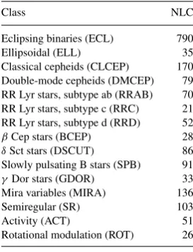
Table 1. The variability classes taken into account in the multistage tree, with the number of light curves (NLC) used to define the classes.

Class NLC

Eclipsing binaries (ECL) 790

Ellipsoidal (ELL) 35

Classical cepheids (CLCEP) 170 Double-mode cepheids (DMCEP) 79 RR Lyr stars, subtype ab (RRAB) 70 RR Lyr stars, subtype c (RRC) 21 RR Lyr stars, subtype d (RRD) 52

βCep stars (BCEP) 28

δSct stars (DSCUT) 86

Slowly pulsating B stars (SPB) 91

γDor stars (GDOR) 33

Mira variables (MIRA) 136

Semiregular (SR) 103

Activity (ACT) 51

Rotational modulation (ROT) 26

Figure 1. Gaussian mixture in the two-parameter space (log (ν1), log (a)) for the classical Cepheids in the training set estimated by the expectation-maximization

very far from the class centres in attribute space. For that reason it is important to include an outlier detection step to flag possible wrong predictions. Debosscher et al. (2009) approximated a training class with a single Gaussian, and computed the Mahalanobis distance of a target to the centre of the class as an outlier indicator. For the multistage approach with multidimensional Gaussians, we use the

following extension of the Mahalanobis distance:

d=(_a−_μ) −1(_a−_μ)_, (6)

withathe attribute vector of the target andμthe centre of mass of the Gaussian mixture. The total variance is defined as the sum of

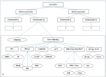
Figure 2. Multistage decomposition. The subtree represented in the S box is not replicated for simplicity.

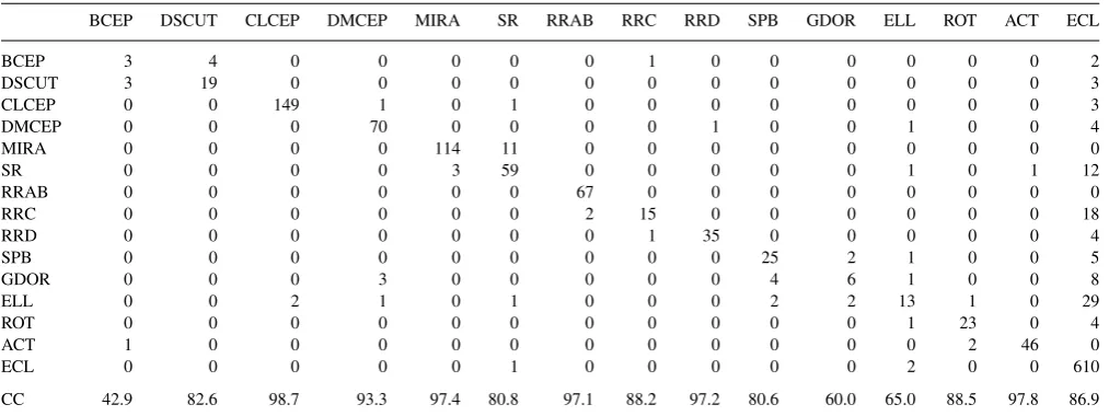
Table 2. The confusion matrix for the multistage tree applied on the training set objects with at least two harmonics for the first frequency. Each stellar variability class in each node is modelled by a finite sum of multivariate Gaussians. The last line lists the correct classification (CC) for every class separately. The average correct classification is 94.2 per cent.

BCEP DSCUT CLCEP DMCEP MIRA SR RRAB RRC RRD SPB GDOR ELL ROT ACT ECL

BCEP 5 3 0 0 0 0 0 0 0 0 0 0 0 0 0

DSCUT 2 19 0 0 0 0 0 1 0 0 0 0 0 0 0

CLCEP 0 0 147 0 0 1 0 0 0 0 0 0 0 0 0

DMCEP 0 0 1 71 0 0 0 0 0 0 0 0 0 0 1

MIRA 0 0 0 0 109 5 0 0 0 0 0 0 0 0 0

SR 0 0 0 0 8 61 0 0 0 0 0 2 1 0 1

RRAB 0 0 0 0 0 0 67 0 0 0 0 0 0 0 0

RRC 0 0 0 0 0 0 2 13 0 0 0 0 0 0 0

RRD 0 0 0 0 0 0 0 0 34 0 0 0 0 0 0

SPB 0 0 0 0 0 0 0 0 0 19 3 1 0 0 0

GDOR 0 0 0 3 0 0 0 0 0 6 6 0 0 0 1

ELL 0 0 0 1 0 1 0 0 1 0 1 13 0 0 9

ROT 0 0 0 0 0 0 0 0 0 0 0 0 22 0 1

ACT 0 0 0 0 0 0 0 0 0 0 0 0 0 46 0

ECL 0 1 3 0 0 5 0 3 1 6 0 4 3 1 690

the intracomponent variances and the intercomponent variance:

≡ 1

Nc Nc

k=1

k+ 1

Nc Nc

k=1

(μk−μ)(μk−μ), (7)

whereμk is the mean vector of each of theNc Gaussian compo-nents. If, and only if, the distance is above a certain threshold, the outlier flag will be set to indicate that the target does not seem to belong to any of the pre-defined classes. This distance is a multidi-mensional generalization of the one-dimultidi-mensional statistical distance (e.g. distance to a mean value of a Gaussian in terms of the standard deviation). For this reason, a value of the distance thresholdd=3 is chosen.

2.4 Training the classifier

In order to train the classifier, we computed the attributes of the training set objects, which were taken fromHipparcos, OGLE and

CoRoT, with the variability detection pipeline, described in Sec-tion 2.1. We only computed up to two significant frequencies with each up to three harmonics, which in our experience is sufficient for classification purposes. Since the quality of the classification results depends crucially on the quality of the training set, we checked all the light curves and phase plots in this set. The variability classes we took into account are listed in Table 1. We carefully set up the multistage tree, which is given in Fig. 2. Applying clustering tech-niques onCoRoTdata, Sarro et al. (2009) managed to identify new classes. In view of theKeplermission, two of these classes, stars with activity and variables due to rotational modulation, are taken into account in the multistage tree. A detailed description of these two classes can be found in Debosscher et al. (2010).

In each node, we manually selected the best attributes to distin-guish the classes considered in that node. In order to evaluate the significance of an attribute we measured the information gain and gain ratio with respect to each class (Witten & Frank 2005). Based on these results we selected the best attributes in terms of highest

Table 3. The confusion matrix for the multistage tree applied on the training set objects with at least two harmonics for the first frequency. Each stellar variability class in each node is modelled by a single Gaussian. The last line lists the correct classification (CC) for every class separately. The average correct classification is 92.7 per cent.

BCEP DSCUT CLCEP DMCEP MIRA SR RRAB RRC RRD SPB GDOR ELL ROT ACT ECL

BCEP 5 3 0 0 0 0 0 0 0 0 0 0 0 0 0

DSCUT 1 18 0 0 0 0 0 0 0 0 0 0 0 0 0

CLCEP 0 0 148 0 0 1 0 0 0 0 0 0 0 0 1

DMCEP 0 0 0 71 0 0 0 0 0 0 0 1 0 0 2

MIRA 0 0 0 0 114 10 0 0 0 0 0 0 0 0 0

SR 0 0 0 0 3 55 0 0 0 0 0 0 0 0 14

RRAB 0 0 0 2 0 0 67 0 0 0 0 0 0 0 0

RRC 1 0 0 0 0 0 2 14 0 0 0 0 0 0 1

RRD 0 0 0 0 0 0 0 0 32 0 0 0 0 0 0

SPB 0 0 0 0 0 0 0 0 0 19 2 1 0 0 0

GDOR 0 0 0 2 0 0 0 0 0 7 8 0 0 0 2

ELL 0 0 1 0 0 1 0 0 0 1 0 15 0 0 15

ROT 0 0 0 0 0 2 0 0 0 1 0 0 23 0 1

ACT 0 0 0 0 0 0 0 0 0 0 0 0 0 47 0

ECL 0 2 2 0 0 4 0 3 4 3 0 3 3 1 666

CC 71.4 78.3 98.0 94.7 97.4 75.3 97.1 82.4 88.9 61.3 80.0 75.0 88.5 100.0 94.8

Table 4. The confusion matrix for a single-stage classifier applied on the training set objects with at least two harmonics for the first frequency. Each stellar variability class is modelled by a single Gaussian. The last line lists the correct classification (CC) for every class separately. The average correct classification is 89.3 per cent.

BCEP DSCUT CLCEP DMCEP MIRA SR RRAB RRC RRD SPB GDOR ELL ROT ACT ECL

BCEP 3 4 0 0 0 0 0 1 0 0 0 0 0 0 2

DSCUT 3 19 0 0 0 0 0 0 0 0 0 0 0 0 3

CLCEP 0 0 149 1 0 1 0 0 0 0 0 0 0 0 3

DMCEP 0 0 0 70 0 0 0 0 1 0 0 1 0 0 4

MIRA 0 0 0 0 114 11 0 0 0 0 0 0 0 0 0

SR 0 0 0 0 3 59 0 0 0 0 0 1 0 1 12

RRAB 0 0 0 0 0 0 67 0 0 0 0 0 0 0 0

RRC 0 0 0 0 0 0 2 15 0 0 0 0 0 0 18

RRD 0 0 0 0 0 0 0 1 35 0 0 0 0 0 4

SPB 0 0 0 0 0 0 0 0 0 25 2 1 0 0 5

GDOR 0 0 0 3 0 0 0 0 0 4 6 1 0 0 8

ELL 0 0 2 1 0 1 0 0 0 2 2 13 1 0 29

ROT 0 0 0 0 0 0 0 0 0 0 0 1 23 0 4

ACT 1 0 0 0 0 0 0 0 0 0 0 0 2 46 0

ECL 0 0 0 0 0 1 0 0 0 0 0 2 0 0 610

information gain and gain ratio, which make sense from an astro-physical point of view. In practice ‘random’ attributes can show structure, even if they are not supposed to. The attributes we know by theory that should be random variables were excluded in order to avoid overfitting. In each node the classifier was then tested using stratified 10-fold cross-validation (see e.g. Witten & Frank 2005). In stratifiedn-fold cross-validation, the original sample is randomly partitioned intonsubsamples. Of thensubsamples, a single one is retained as the validation data for testing the model, and the remain-ingn−1 subsamples are used as training data. The cross-validation process is then repeatedntimes (the folds), with each of then sub-samples used exactly once as the validation data. Then thenresults from the folds are combined to produce a single estimation. Each fold contains roughly the same proportions of the class labels. We kept the attributes giving the best classification results, not only in terms of correctly classified targets, but also in terms of accu-racy measured by the area under the ROC curve (Witten & Frank 2005). The higher the area under the ROC curve, the better the test is.

Stratified 10-fold cross-validation was also applied on the mul-tistage tree as a whole. When only the first frequency and its main amplitude are available, poor results are obtained because there is simply too little information available for classification. When we leave out those examples and only use the training examples for which we have more information, very good results are ob-tained as can be seen in Table 2. Only 5.8 per cent of the training examples is wrongly classified. When we replace the variability classes models by single Gaussians, we have a worse result with 7.3 per cent of wrong predictions (see Table 3). When we also use only one stage, 10.7 per cent of the training examples are mis-classified (see Table 4). We can thus conclude that our multistage classification tree with Gaussian mixtures at its nodes is a significant improvement.

3 A P P L I C AT I O N T O T R E S DATA

3.1 The TrES Lyr1 data set

We analysed 25 947 light curves in the TrES Lyr1 field. TrES is a network of three 10-cm optical telescopes searching the sky for transiting planets (Alonso et al. 2007; O’Donovan 2008). This network consisted of Sleuth (Palomar Observatory, Southern Cal-ifornia), the PSST (Lowell Observatory, Northern Arizona) and STARE (Observatorio del Teide, Canary Islands, Spain), as TrES now excludes Sleuth and STARE, but includes WATTS. The TrES Lyr1 field is a 5◦.7×5◦.7 field, centred on the star 16 Lyr and is part of theKepler field (Alonso et al. 2007). Most light curves have about 15 000 observations spread with a total time-span

Table 5. Overview of the classification results using two dif-ferent cut-off values for the highest class probabilityp. A generalized Mahalanobis distanced<3 to the most probable class is taken as defined in equation (6).

Class(es) p>0.5 p>0.75

Eclipsing binaries (ECL) 158 130

Ellipsoidal (ELL) 571 214

Classical cepheids (CLCEP) 3 2

Double-mode cepheids (DMCEP) 0 0

RR-Lyr stars, subtype ab (RRAB) 2 2

RR-Lyr stars, subtype c (RRC) 4 4

RR-Lyr stars, subtype d (RRD) 0 0

βCep orδSct stars (BCEP/DSCUT) 842 720 SPB orγDor stars (SPB/GDOR) 914 453

Mira variables (MIRA) 0 0

Semiregular (SR) 8 5

of approximately 75 d. A small fraction has less than 5000 ob-servations with a total time-span of around 62 d. Obob-servations are given in either the Sloan r (Sleuth) or the Kron–Cousins R magnitude (PSST) and the meanRmagnitude ranges from 9.2 to 16.3.

3.2 Classification of variable stars

3.2.1 Results of the variability detection

With the use of the variability detection algorithm, described in Section 2.1, we searched for frequencies in the range 3/Ttot to 50

c/d, with Ttot the total time-span of the observations in days. In

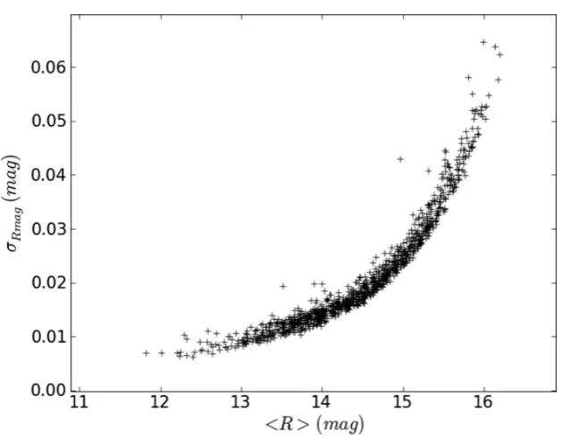
order to avoid the problem of daily aliasing in an automated way, small frequency intervals around multiples of 1 c/d were flagged as ‘unreliable’. Using a false alarm probability ofα=0.005 (the null hypothesis of only having noise in the light curves is rejected when P< α, withPthe probability of finding such a peak in the power spectrum of a time series that only contains noise), about 18 000 objects were found non-constant. The stars for which we could not

find significant frequencies were used to determine the rms level of the time series as a function of the mean magnitude, which is plotted in Fig. 3, indicating to what level we can detect variability. The upward trend can be explained in terms of photon noise.

3.2.2 Classification results

We used the multistage tree presented in Section 2.4, where we excluded the stars with activity and variables with rotational mod-ulation. As already mentioned, these classes were included in the multistage tree in view of theKeplermission. However, we do not expect to find good candidates in the ground-based data of TrES Lyr1 as these classes are characterized by low amplitudes. The clas-sification algorithm was able to detect many good candidate class members. By candidate we mean a target belonging to the class with the highest class probability above two different cut-off values pmin=0.5 and 0.75 and with a generalized Mahalanobis distance

d< 3 to that class. A quick visual check of the light curves and phase plots of the targets with a distance above 3 showed that a

large fraction of light curves suffers from instrumental effects. The results of the classification are listed in Table 5.

As withCoRoT, the main objective of TrES was the search for planets. We do not find many long period variables, Cepheids and RR Lyr among its targets. The total time-span of the light curves is also too short to be able to detect Mira type variables.

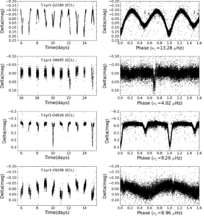
3.2.3 Eclipsing binaries and ellipsoidal variables

Irrespective of the observed field on the sky, we should always find a number of eclipsing binaries and ellipsoidal variables. Light curves of eclipsing binaries are very different from those of pulsating stars and therefore generally well separated using the phase differences between the first three harmonics of the first frequency. Most de-tected candidate binaries have therefore a very high probability (>90 per cent) of belonging to the ECL class. We found about 158 reliable eclipsing binaries. Some good examples of eclipsing binary light curves are shown in Fig. 4. It is remarkable that, although

eclipses are not always easily seen in the light curve, they clearly show up in the phase plot and are detected by the classification algorithm.

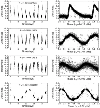
3.2.4 Monoperiodic pulsators

Despite the fact that Cepheids and RR Lyr are easy to distinguish from other classes due to their large amplitudes, almost no good candidates were found. Examples of the few candidates found are shown in Fig. 5.

3.2.5 Multiperiodic pulsators

As no colour information was available, confusion betweenβCep andδSct stars occurs, because of overlapping frequency ranges. For this reason we merged these two classes into a single class. It is possible that, for the same target, these classes have similar

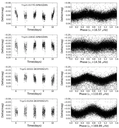
Figure 6. Left-hand column: some TrES Lyr1 light curves of non-radial pulsators. Right-hand column: the corresponding phase plots, made with the detected frequency.

probabilities below 0.5, but add up to a value well above 0.5. Sim-ilarly, we could often not make a clear distinction betweenγ Dor and SPB stars, because they show similar gravity-mode spectra. This problem may be solved by adding supplementary information like temperature, colours or a spectrum, not only for the targets but also for the training sets. Although frequencies around multiples of 1 c/d have been set unreliable, especially theγDor and SPB classes suffer from the combination of daily aliasing and instrumental ef-fects. For this class, a visual inspection of the light curves and phase plots was needed. Fig. 6 shows some good examples of non-radial pulsators.

4 D I S C U S S I O N A N D C O N C L U S I O N S

In contrast to previous classification methods for time series of photometric data (e.g. Debosscher et al. 2007) we now only use significant frequencies and overtones as attributes, giving rise to

less confusion. We are able to statistically deal with a variable number of attributes using the multistage approach developed here. Another advantage of this approach is that the conditional prob-abilities in each node can be simplified by dropping one or more attributes that are not relevant for a particular node. Moreover, in each node, a different classifier can be chosen. In this paper we only used the Gaussian mixture classifier, but also other methods like e.g. Bayesian nets can be used, which gives more flexibility. Finally, the variability classes were better described by a finite sum of multivariate Gaussians.

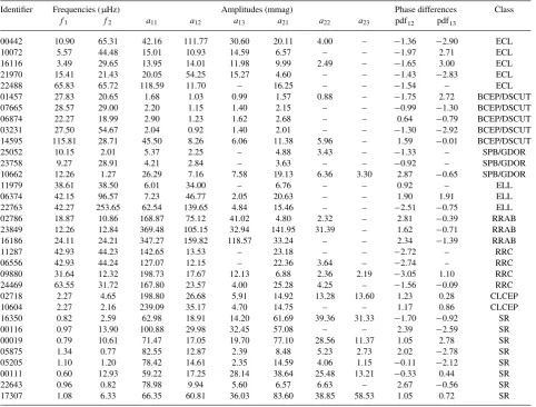
Table 6. The results of the supervised classification applied to the TrES Lyr1 data base. The first column contains the identifiers of the TrES Lyr1 objects. For each object, the first two frequencies, each with three harmonics, are given. Phase differences for the first frequency are also given. Details of these attributes can be found in Debosscher et al. (2007). The last column gives the most probable class according to the classification. The full version of this table is available with the online version of the article (see Supporting Information).

Identifier Frequencies (µHz) Amplitudes (mmag) Phase differences Class

f1 f2 a11 a12 a13 a21 a22 a23 pdf12 pdf13

00442 10.90 65.31 42.16 111.77 30.60 20.11 4.00 – −1.36 −2.90 ECL

10072 5.57 44.48 15.01 10.93 14.59 6.57 – – −1.97 2.71 ECL

16116 3.49 29.65 13.95 14.01 11.98 9.99 2.49 – −1.65 3.00 ECL

21970 15.41 21.43 20.05 54.25 15.27 4.60 – – −1.43 −2.83 ECL

22488 65.83 65.72 118.59 11.70 – 16.25 – – −1.54 – ECL

01457 27.83 20.65 1.68 1.03 0.99 1.57 0.88 – −1.75 2.72 BCEP/DSCUT

07665 28.57 29.00 2.20 1.15 1.40 2.15 – – −0.99 −1.30 BCEP/DSCUT

06874 22.27 18.99 2.90 1.23 1.62 2.68 – – 0.64 −0.79 BCEP/DSCUT

03231 27.50 54.67 2.04 0.92 1.40 2.01 – – −1.30 −2.92 BCEP/DSCUT

14595 115.81 28.71 45.50 8.26 6.06 11.38 5.96 – 1.59 −0.01 BCEP/DSCUT

25052 10.15 2.01 5.37 2.25 – 4.88 3.43 – −1.33 – SPB/GDOR

23758 9.27 28.91 4.21 2.84 – 3.63 – – −0.92 – SPB/GDOR

10662 12.26 1.27 26.29 7.16 7.58 19.13 6.36 3.30 2.87 −0.65 SPB/GDOR

11979 38.61 38.50 6.01 34.00 – 6.76 – – 0.92 – ELL

06374 42.15 96.57 7.23 46.77 2.05 20.63 – – 1.90 1.91 ELL

22763 42.27 253.65 62.54 139.65 4.84 15.46 – – −2.51 −0.75 ELL

02786 18.87 10.86 168.87 75.12 41.02 4.80 2.32 – 2.81 −0.39 RRAB

23849 12.26 12.84 369.48 105.15 32.94 141.95 31.39 – 1.62 −0.71 RRAB

16186 24.11 24.21 347.27 159.82 118.57 33.24 – – 2.34 −1.39 RRAB

11287 42.93 44.23 142.65 13.53 – 23.18 – – −2.72 – RRC

06556 42.93 44.24 127.07 12.15 – 22.36 3.64 – −2.74 – RRC

09880 31.64 12.32 198.73 17.67 12.13 6.88 2.36 2.19 −3.05 1.10 RRC

24469 63.55 31.72 167.80 23.57 4.00 25.28 4.25 – −1.56 −0.09 RRC

02718 2.27 4.65 198.80 26.68 5.91 14.92 13.28 13.60 1.23 0.28 CLCEP

10604 2.27 2.16 239.09 35.17 4.70 14.75 – – 1.17 0.86 CLCEP

16350 0.82 2.59 62.98 18.91 14.20 61.69 39.36 31.33 −1.70 −0.92 SR

00116 0.97 13.90 100.88 29.98 32.45 57.08 – – 2.39 −2.59 SR

00019 0.79 10.61 71.47 17.05 19.70 77.10 28.56 11.37 1.05 2.78 SR

05875 1.34 0.77 82.55 12.87 2.39 8.48 5.23 2.73 2.02 −2.78 SR

05205 1.10 1.20 78.42 14.61 2.35 14.59 4.06 1.15 −0.11 −2.12 SR

00111 0.60 12.93 59.22 17.25 28.14 38.64 25.48 13.21 −0.33 0.44 SR

22643 0.96 0.82 78.98 9.94 5.60 6.57 6.63 – 2.67 −0.56 SR

17307 1.08 6.33 66.35 60.81 36.03 83.60 38.85 58.53 1.05 0.72 SR

non-radial pulsators we also mention the detection of binary stars and some classical radial pulsators. The results of this classification will be made available through electronic tables. A small sample is given in Table 6. See the Supporting Information for the full results.

AC K N OW L E D G M E N T S

The research leading to these results has received funding from the European Research Council under the European Community’s Sev-enth Framework Programme (FP7/2007-2013)/ERC grant agree-ment no. 227224 (PROSPERITY), the Research Council of K. U. Leuven (GOA/2008/04), from the Fund for Scientific Research of Flanders (G.0332.06), the Belgian Federal Science Policy Of-fice (C90309: CoRoT Data Exploitation, C90291 Gaia-DPAC) and the Spanish Ministerio de Educaci´on y Ciencia through grant AYA2005-04286. Public access to the TrES data was provided to the through the NASA Star and Exoplanet Database (NStED, http://nsted.ipac.caltech.edu).

R E F E R E N C E S

Aerts C., Christensen-Dalsgaard J., Kurtz D. W., 2010, Asteroseismology. Springer-Verlag, Berlin (ISBN 978-1-4020-5178-4)

Alonso R. et al., 2007, in Afonso C., Weldrake D., Henning Th., eds, ASP Conf. Ser. Vol. 366, Transiting Extrasolar Planets Workshop. Astron. Soc. Pac., San Francisco, p. 13

Debosscher J. et al., 2007, A&A, 475, 1159 Debosscher J. et al., 2009, A&A, 506, 519

Debosscher J., Blomme J., Aerts C., De Ridder J., 2010, A&A, submitted

Fridlund M., Baglin A., Lochard J., Conroy L., 2006, eds, ESA SP-1306, The CoRoT Mission: Pre-Launch Status. ESA, Noordwidjk

Gamerman D., Migon H., 1993. J. R. Statistical Soc. Ser. B, 55, 629 Gilliland R. L. et al., 2010, PASP, 122, 131

Horne J. H., Baliunas S. L., 1986, ApJ, 302, 763

O’Donovan F., 2008, PhD thesis, California Institute of Technology, Pasadena, California

Sarro L. M., Debosscher J., L´opez M., Aerts C., 2009, A&A, 494, 739 Schwarzenberg-Czerny A., 1998, MNRAS, 301, 831

S U P P O RT I N G I N F O R M AT I O N

Additional Supporting Information may be found in the online ver-sion of this article:

Table 6.The results of the supervised classification applied to the TrES Lyr1 data base.

Please note: Wiley-Blackwell are not responsible for the content or functionality of any supporting materials supplied by the authors. Any queries (other than missing material) should be directed to the corresponding author for the article.