Identifcation of correlation between 3D surfaces using data mining techniques: a case study of predicting springback in sheet metal forming

(1)

Data Mining Techniques: A Case Study of Predicting

Springback in Sheet Metal Forming

Thesis submitted in accordance with the requirements of the University of Liverpool for the degree of Doctor in Philosophy

by

Subhieh El Salhi

Faculty of Science

Department of Computer Science

(2)

(3)

Din Al Salhi, my greatest inspiration of all.

(4)

This thesis presents data mining research work undertaken in the context of identi-fying correlations between 3D surfaces. More specifically, this research is directed at predicting distortions (referred to as springback) in sheet metal forming. The main ob-jective was to identify a mechanism that “best” serves to both capture effectively 3D geometrical information while at the same time allowing for the generation of effective predictors (classifiers). To this end, three distinct 3D surface representation techniques are proposed based on three different concepts. The first technique, the Local Geom-etry Matrices (LGM) representation, is founded on the idea of Local Binary Patterns (LBPs), as used with respect to image texture analysis, whereby surfaces are defined in terms oflocal neighbourhoodssurrounding individual points in a 3D surface. The second technique, the Local Distance Measure (LDM) representation, is influenced by the obser-vation that springback is greater further from edges and corners, consequently surfaces are defined in terms of distance to the nearest edge or corner. The third technique, the Point Series (PS) representation, is founded on the idea of using a spatial “linearisation” with which to represent surfaces in terms of point series curves. The thesis describes and discusses each of these in detail including, in each case, the theoretical underpin-ning supporting each representation. A full evaluation of each of the representations is also presented. As will become apparent, the PS technique was found to be the most effective. The presented evaluation was directed at predicting springback, in the context of the Asymmetric Incremental Sheet Forming (AISF) manufacturing process, in such a way that an enhanced version of the desired 3D surface can be proposed intended to minimise the effect of springback. For the evaluation two flat-topped, square-based, pyramid shapes were used. Each pyramid had been manufactured twice using Steel and twice using Titanium. In addition this thesis presents some idea on how the springback prediction mechanism can be incorporated into an “intelligent process model”. The evaluation of this model, by manufacturing corrected shapes, established that a sound prediction framework, incorporating the 3D surface representation techniques espoused in this thesis coupled with a compatible classification technique, had been established.

(5)

This thesis is the end of my three year journey to get my Ph.D degree in Computer Science. First and foremost, all praise be to Allah, the Most Gracious and Most Merciful, for giving me the power, the strength and the patience to overcome all tests that came my way and for blessing me with those wonderful people who have believed that my efforts will be fruitful by the end of my Ph.D journey.

I am deeply indebted to my Supervisor, Professor Frans Coenen, who has offered me the chance to work under his supervision and who has supported me with his invaluable assistance, care and guidance throughout my Ph.D research. He has been always there to listen, discuss and suggest research ideas. Through his extraordinary experience, he has taught me not only to be a good student but also a good researcher and an intellectual person. He has enlightened my way by his inspiration and endless efforts on how to explain and present academic work simply and clearly. He has been always not only a great mentor but also a real friend. He was the most perfect resource which inspired me and enriched my experience making me the person that I am today. He was the best supervisor any one could hope for, and more. It has been a pleasure and an honour to have been supervised by him.

My deepest appreciation and gratitude to my second supervisor Dr. Clare Dixon for her assistance, constructive suggestions, insightful comments, feedback and research ideas. Besides my supervisors, I would also like to extend my gratitude to my assessor committee; Professor Trevor J.M. Bench-Capon, Dr. Boris Konev and Dr. Muhammad Khan for their evaluation, constructive comments and feedbacks. I would also like to thank staff at Tecnalia (Spain) and IBF (Germany) for their support in providing test data and the manufacturing of corrected shapes, in particular: Dr. Mariluz Penalva Oscoz and Dr. Asun Rastrero from Tecnalia, and David Baily from IBF.

Beside the facilities that have been provided by the Department of Computer Science, the kindness of people that characterises the department to be the perfect place to work in, I am also grateful to the staff at the department for helping me in numerous ways. Thanks also go to my fellow PhDs who stood by my side, provided me with incredible support and have been always there for me when I needed them. In particular, Puteri N. E. Nohuddin, Matias Fernando Garcia, Kwankamon Dittakan, Wen Yu, Latifa Al-Abdulkarim, Maduka Attamah, Jeffery Raphael and Eric Schneider.

It is very difficult for me to find the right words to express my gratitude to my parents, Dr. “Moh’d Faraj” Al Salhi and Basema Abu Zer. They not only have raised

(6)

Without their support and encouragement, this work would not have been started. I would like also to thank my sisters and brothers; Mayssa, Amer, Shaima, Fatima, Alaa El Deen, Alaa and Leena for their faith in me and my ability to accomplish my Ph.D tasks professionally and also for their continuous love and respect.

My literary skills are powerless to express my respect, love and appreciation to my husband, Moneef Al Qaisi for the patience, support and persistent confidence he provided me with. He has been always my best friend my confidant and my role model. I am blessed to share my life with him. His love and kindness are foundation stones for all that I am and currently have.

My sincere acknowledgements would not be complete without true thanks to my angels Khaled, Tala and Ahmad. I am blessed to have such wonderful kids in my life. I could not have coped with the pressures of life without their love and hugs. I owe them so much; they have always inspired me to work harder, smarter and to utilise my time effectively. They have always been the source of my strength to keep reaching for the best. I hope that they will be proud of me when they realize what my Ph.D years have entailed.

(7)

Abstract iv

Acknowledgements v

1 Introduction 1

1.1 Overview . . . 1

1.2 Motivation . . . 3

1.3 Research Question and Related Issues . . . 4

1.4 Contributions . . . 6

1.5 Research Methodology . . . 7

1.6 Published Work . . . 8

1.7 Thesis Organisation . . . 10

1.8 Summary . . . 11

2 Background, Related Work and The Application Domain 12 2.1 Introduction . . . 12

2.2 Application Domain: Asymmetric Incremental Sheet Forming (AISF) . . 13

2.2.1 Overview of Springback . . . 14

2.3 Knowledge Representation and Data Mining . . . 18

2.3.1 Decision Tree . . . 19

2.3.2 Rule-Based Classifiers . . . 22

2.3.3 Bayesian Classifiers . . . 24

2.3.4 Artificial Neural Network . . . 25

2.3.5 k-Nearest Neighbour . . . 27

2.3.6 Dynamic Time Warping (DTW) . . . 28

2.4 3D Surface Representation Techniques . . . 33

2.4.1 Mathematical Representation . . . 33

Parametric Representations . . . 34

Implicit Representations . . . 35

2.4.2 Mesh (Polygonisation) Representations . . . 36

2.4.3 Other 3D Surface Representation Techniques . . . 37

2.4.4 Overview of Critical Feature Techniques . . . 38

2.5 Evaluation Criteria . . . 40

2.6 Summary . . . 42

(8)

3.1 Introduction . . . 44

3.2 The Representation and Springback Prediction (RASP) Framework . . . . 45

3.3 Grid Representation . . . 46

3.4 Springback Calculation Mechanism . . . 47

3.4.1 Normal Calculation . . . 48

3.4.2 Intersection Point Calculation . . . 48

3.4.3 Error (Springback) Calculation . . . 51

3.5 Discretising process . . . 54

3.6 Evaluation Data Sets . . . 55

3.7 Summary . . . 59

4 Local Geometry Matrix Representation (LGM) 62 4.1 Introduction . . . 62

4.2 The Local Geometry Matrix (LGM) . . . 63

4.3 Experiments and Evaluation . . . 67

4.3.1 Identifying whether the δz or θ LGM representation is the most effective . . . 68

4.3.2 Identification of the best value ford(grid size) . . . 68

4.3.3 Identification of best label size (|L|) . . . 69

4.3.4 Identification of the best LGM model . . . 72

4.3.5 Identification of the most appropriate classification algorithms . . 72

4.3.6 Training and testing the classifier on a different data set . . . 75

4.3.7 Run Time Analysis . . . 76

4.4 Summary . . . 78

5 Local Distance Measure (LDM) Representation 80 5.1 Introduction . . . 80

5.2 Effect of proximity of Critical Points on Springback . . . 81

5.3 The LDM Mechanism . . . 83

5.3.1 Critical Point Detection . . . 83

5.3.2 Distance Calculation . . . 86

5.4 LDM Detailed Examples . . . 88

5.5 Combining The LDM Model with The LGM Model . . . 90

5.6.1 Best value forξ . . . 92

5.6.2 Identification of the best value ford(grid size) . . . 92

5.6.3 Best number of labels (|L|) . . . 93

5.6.4 Best LDM model . . . 94

5.6.5 Training and testing the classifier on a different data sets . . . 95

5.7 Run Time Analysis . . . 97

5.8 Summary . . . 100

6 Point Series Representation 103 6.1 Introduction . . . 103

6.2 Point Series Representation . . . 104

6.3 The Prediction Framework Mechanism . . . 105

(9)

6.4 Evaluation . . . 112

6.4.1 Discretised vs Real Point Series Representation . . . 113

6.4.2 The Effect of Grid Size . . . 114

6.4.3 The Effect of Neighbourhood Size . . . 117

6.4.4 The Nature of the Linearisation: all Points vs key Points Repre-sentation . . . 119

6.4.5 Generalisation . . . 119

6.5 Run Time Evaluation . . . 121

6.6 Summary . . . 123

7 Statistical Comparison Between the Proposed 3D Representations 126 7.1 Overview of Statistical Performance Comparison . . . 126

7.2 Friedman Statistical Test . . . 127

7.3 Using the Same Data Set for Statistical Comparison . . . 130

7.4 Using Different Data Sets for Statistical Comparison . . . 132

7.6 Summary . . . 135

8 Identified Springback Error Application 138 8.1 Introduction . . . 138

8.2 Corrected Cloud Generation Mechanism . . . 139

8.3 Evaluation of Formed Parts . . . 141

8.3.1 Steel Manufactured Shapes (GS and MS) . . . 141

8.3.2 Titanium Based Shapes . . . 147

8.4 Summary . . . 147

9 Intelligent Process Model 149 9.1 Introduction . . . 149

9.2 Single Pass IPM . . . 149

9.3 Iterative IPM . . . 151

9.6 Summary . . . 159

10 Conclusion and Future Research Works 162 10.1 Inroduction . . . 162

10.2 Summary . . . 162

10.3 Main Findings and Contributions . . . 164

10.4 Future Work . . . 166

A Error Visualisation for Gonzalo and Modified Pyramids 168 B Discretised Results for PS Representation Technique 186 C AUC Calculation based on Mann-Whitney-Wilcoxon. 191

(10)

References 198

(11)

2.1 The main themes of the Thesis: Sheet Metal Forming (AISF in particular),

Data Mining (classification in particular) and 3D Surface Representation. . . 12

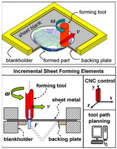
2.2 The AISF process. The basic elements of AISF are the metal forming force F, the tool speedv and the spin angular speed w. [114]. . . 14

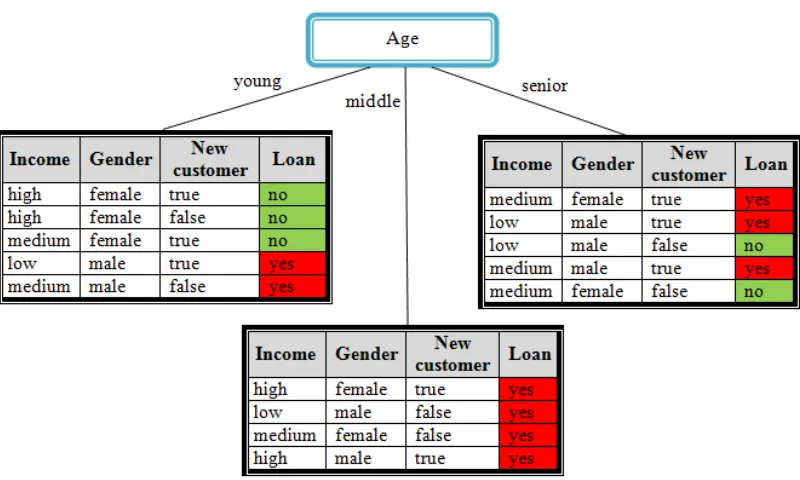
2.3 The three subsets of the data set Dobtained after splitting with respect to the different attribute values: young,middle and senior. . . 22

2.4 The DT classifier for the data setD presented earlier in Table 2.1. . . 23

2.5 A typical Perceptron Example. . . 26

2.6 A warping path, P, that satisfies the (i) Boundary, (ii) Monotonicity and (iii) Step size conditions. . . 29

2.7 A warping path, P where theboundary condition is violated. . . 29

2.8 A warping path, P where themonotonicity condition is violated. . . 29

2.9 A warping path, P where thestep size condition is violated. . . 29

2.10 Different warping paths can be defined between two point series A and B. Theoptimal warping path is in red colour. The distance values stored in the adjacent cells {M(i−1, j), M(i, j−1), M(i−1, j−1)} (shaded block) are used to identify the value ofM(i, j) elements (black and red points). . . 32

2.11 An example of the Sakoe-Chiba band windowing concept withw = 3. Only the shaded elements are considered when determining the optimum warping path. . . 32

2.12 A parametric surface. . . 34

2.13 Confusion matrix. . . 41

2.14 Four different example ROC curves (A, B, C and D). Curve C is the curve produced as a result of simply guessing. Curve A is said to dominate B, C and D since A is above and to the left of B, C and D. However, B and D do not dominate each other therefore the AUC is a convenient way to compare their performance [135]. . . 43

3.1 Schematic describing the Representation And Springback Prediction (RASP) Framework. . . 45

3.2 Typical grid structure for a point cloud (red grid centres indicate the corner grid squares). . . 47

3.3 ~v and~u vector configurations, indicated in red, that maybe used for normal calculation. Note that a clockwise direction is used so that all normals point in the same direction. . . 49

3.4 Error (springback) calculation (E) between Gin and Gout defined as the distance between the pointPi onGin to where the normal ofPi cutsGout at Pint. . . 50

(12)

angle between them is (θ = 180◦). Therefore, the error E, in this case, is assigned a negative (−) sign. However, the angle between the normal~nand

−−−→

PiPint on the right hand example is θ= 0◦ which means that both vectors

run parallel in the same direction and as a result the error is assigned a + sign. . . 52 3.6 Gonzalo (left) and Modified (right) Pyramids. . . 57 3.7 Side sections of Gonzalo (left) and Modified (right) Pyramids. . . 57 3.8 Different views for the GSV1Gin point cloud using grid size d= 1mm. . . . 60

3.9 Different views for the MSV1Gin point cloud using grid size d= 1mm. . . . 60

4.1 Level one neighbourhood model. The eight closest surrounding neighbours (Pi coloured in red) for the grid square are considered and represented using

a 3×3 LGM (P0 is the centre point coloured in black). . . 63

4.2 Level two neighbourhood model. The eight surrounding neighbours (Pi

coloured in red) for the grid square that are “one step away” are consid-ered and represented using a 3×3 LGM (P0 is the centre point coloured in

black). . . 63 4.3 The composite model founded on a 5×5 LGM to represent the surrounding

neighbourhood (Pi coloured in red) of P0 coloured in black. . . 64

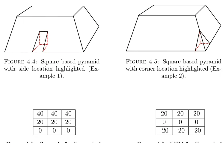
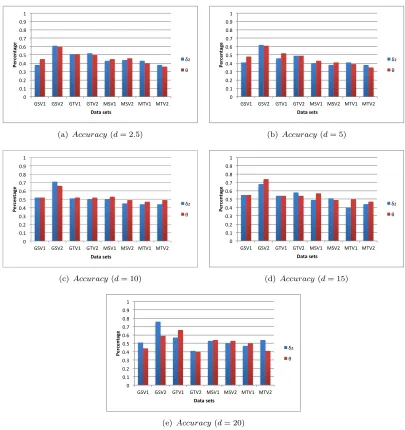
4.4 Square based pyramid with side location highlighted (Example 1). . . 65 4.5 Square based pyramid with corner location highlighted (Example 2). . . 65 4.6 Comparison of theδzandθLGM representations in terms of accuracy, with

respect to the eight test data sets using: different grid sizes, |L| = 3, C4.5 and the composite LGM model. . . 69 4.7 Comparison of the δz and θ LGM representations in terms of AUC, with

respect to the eight test datasets, using: different grid sizes, |L|= 3, C4.5 and the composite LGM model. . . 70 4.8 Comparison of different values ofd in combination with the LGM model in

terms of AUC, with respect to the eight datasets, using: |L|= 3, C4.5 and the composite LGM model coupled withδz values. . . 71 4.9 Comparison of different values of |L| in combination with the LGM model,

in terms of accuracy and AUC, with respect to the eight datasets, using: d= 10, C4.5 and the composite LGM model coupled withδz values. . . 73 4.10 Comparison of the three variations of LGM model, in terms of accuracy and

AUC, with respect to the eight datasets, using: d= 10, |L|= 3, C4.5 and δz values. . . 74 4.11 Comparison of use of different classifiers with the LGM model, in terms of

accuracy and AUC, with respect to the eight datasets, usingd= 10,|L|= 3 C4.5 and the composite LGM model coupled withδz values. . . 75

(13)

and C4.5 classification algorithm. . . 77

4.13 The run time for d= 2.5 for the different data sets. . . 78

4.14 The run time for d= 5 for the different data sets. . . 78

5.1 An example shape represented in terms of a point cloud. . . 81

5.2 Colour coding used in Figure 5.3. . . 82

5.3 2D-plot showing springback distribution over a shape (MSV1): (a) magni-tude only, (b) magnimagni-tude and direction (d= 2.5). . . 82

5.4 The effect of different d values on critical point detection using ξ = 9 and the GSV1 data set. . . 85

5.5 The effect of different ξ values on critical point detection usingd= 2.5 and the GSV1 data set. . . 86

5.6 Region growing example using Algorithm 5.2 where the closest critical point is located within the level two neighbourhood. . . 87

5.7 Example of a hemisphere shape for a given point p0 with four Level one neighbourhood pointsp1,p2,p3and p4 each associated with its own normal, ~ n1,n~2,n~3 and n~4 respectively. . . 89

5.8 Accuracy and AUC results obtained for the LDM model, using different values for d with respect to the eight test datasets (using |L| = 3 and the C4.5 classification algorithm). . . 93

5.9 Accuracy and AUC results obtained for the LDM model using different values for|L|with respect to the eight evaluation datasets (using d= 2.5 and the C4.5). . . 94

5.10 AUC and Accuracy results to identify the best LDM model using|L|= 3 and a range of grid size{2.5,5,10} with respect to the eight evaluation datasets (using the C4.5 classification algorithm). . . 96

5.11 The AUC and Accuracy results produced when generating a classifier on one data set and applying it to another using the LDM model (|L|= 3,d= 2.5 and the C4.5 classification algorithm). . . 98

5.12 The AUC and Accuracy results produced when generating a classifier on one data set and applying it to another using the LDM+ composite LGM model (|L|= 3, d= 10 and the C4.5 classification algorithm). . . 99

5.13 Run time for LDM model using d = {2.5,5,10,15,20} with respect to the eight data sets GSV1, GSV2, GTV1, GTV2, MSV1, MSV2, MTV1 and MTV2.100 5.14 Run time for LDM + composite LGM using d={2.5,5,10,15,20}. . . 101

6.1 Example of a spiral linearisation for a 5×5key PS representation. . . 105

(14)

in shaded area). The indices of the lower and upper boundary are coloured in green. The optimal DTW path is indicated using dark shading with red text. The path commences at M(0,0) and ends at M(11,11). The DTW value is located in M(11,11) and is equivalent to 13 in this case. . . 107 6.3 The AUC and Accuracy results produced when generating a classifier on

one data set and applying it to another using n = 3, the key point PS representation and d= 5. . . 122 6.4 Recorded run time (s) for both theall point and thekey point PS

represen-tation usingn= 3 and d= 5. . . 123 6.5 Recorded run time (s) for both theall point and thekey point PS

represen-tation usingn= 5 and d= 5. . . 123 6.6 Recorded run time (s) for both theall point and thekey point PS

represen-tation usingn= 7 and d= 5. . . 123 6.7 Run time (in seconds) for 3×3 PS representation usingd={2.5,5,10,15,20}

with respect to the eight data sets GSV1, GSV2, GTV1, GTV2, MSV1, MSV2, MTV1 and MTV2. . . 124

7.1 Theχ2 _{distribution. The shaded area is equal to}_α _{and denoted by}_χ2

α, and

represents the region of rejection. The p-value is the area under curve right of the calculatedχ2_F. . . 130 7.2 The average rank (µi) associated with CD value for the classifiers generated

using the same data set. . . 133 7.3 The average rank (µi) associated with CD value for the classifiers generated

using different data sets. . . 135 7.4 The critical values for Chi-Square (χ2) [66]. . . 137

8.1 Corrected Cloud Generation Mechanism. . . 140 8.2 Springback distribution with respect to the shapes manufactured using Cin

cloud (left) and Ccorr (right) for the GS shape and an error scale of ±6 mm. 141

8.3 Springback distribution with respect to the shapes manufactured using Cin

cloud (left) and Ccorr (right) for the GS shape and an error scale of ±4 mm. 142

(left) andCcorr (right) for the GS shape and an error scale of±3 mm. . . 142

(left) andCcorr (right) for the MS shape and an error scale of±6 mm. . . . 143

(left) andCcorr (right) for the MS shape and an error scale of±4 mm. . . . 144

cloud (left) and Ccorr (right) for the MS shape and an error scale of ±3 mm. 144

(15)

8.9 The uncompleted MT shape manufactured up to the point where fractures occurred. . . 148

9.1 Single Pass IPM. . . 150 9.2 Iterative IPM. . . 151 9.3 A average absolute diff values and the average springback distribution of

Cpred for the GSV1 using d= 10 mm. . . 158

9.4 The average absolutediff values and the average springback distribution of Cpred for GSV1 usingd= 1 mm. . . 158

9.7 The average absolutediff values and the average springback distribution of Cpred for GTV1 usingd= 10 mm. . . 159

9.11 The average absolutediff values and the average springback distribution of Cpred for MSV1 using d= 10 mm. . . 160

9.15 The average absolutediff values and the average springback distribution of Cpred for MTV1 usingd= 10 mm. . . 161

9.19 The run time analysis (in seconds) for the eight data sets using d= 10 mm with respect ton= 12 iterations. . . 161

(16)

A.1 The Error scale used to describe both the absolute and the directed error (springback) distribution for the Gonzalo and Modified pyramid shapes. . . . 169 A.2 The absolute error visualisation for the Gonzalo Steel V1 (GSV1) pyramid

for different grid sizes (d). . . 170 A.3 Thedirected error visualisation results for Gonzalo Steel V1 (GSV1) pyramid

for different grid size (d). . . 171 A.4 The absolute error visualisation results for the Gonzalo Steel V2 (GSV2)

pyramid for different grid sizes (d). . . 172 A.5 The directed error visualisation results for the Gonzalo Steel V2 (GSV2)

pyramid for different grid sizes (d). . . 173 A.6 The absolute error visualisation results for the Modified Steel V1 (MSV1)

pyramid for different grid sizes (d). . . 174 A.7 The directed error visualisation results for the Modified Steel V1 (MSV1)

pyramid for different grid sizes (d). . . 175 A.8 The absolute error visualisation results for the Modified Steel V2 (MSV2)

pyramid for different grid sizes (d). . . 176 A.9 The directed error visualisation results for the Modified Steel V2 (MSV2)

pyramid for different grid sizes (d). . . 177 A.10 Theabsoluteerror visualisation results for the Gonzalo Titanium V1 (GTV1)

pyramid for different grid sizes (d). . . 178 A.11 Thedirected error visualisation results for the Gonzalo Titanium V1 (GTV1)

pyramid for different grid sizes (d). . . 179 A.12 Theabsoluteerror visualisation results for the Gonzalo Titanium V2 (GTV2)

pyramid for different grid sizes (d). . . 180 A.13 Thedirected error visualisation results for the Gonzalo Titanium V2 (GTV2)

pyramid for different grid sizes (d). . . 181 A.14 Theabsoluteerror visualisation results for the Modified Titanium V1 (MTV1)

pyramid for different grid sizes (d). . . 182 A.15 Thedirectederror visualisation results for the Modified Titanium V1 (MTV1)

pyramid for different grid sizes (d). . . 183 A.16 Theabsoluteerror visualisation results for the Modified Titanium V2 (MTV2)

pyramid for different grid sizes (d). . . 184 A.17 Thedirectederror visualisation results for the Modified Titanium V2 (MTV2)

pyramid for different grid sizes (d). . . 185

(17)

2.1 A labeled training data set consists of 14 records. Four attributes are used to describe the data set while the Loan attribute used to label the record

with either Yes label (coloured in red) orNo label (coloured in green). . . . 22

3.1 Discretisation Table for a given example. . . 55

3.2 Statistics concerning the width (W) (mm), length (L) (mm), height (H) (mm), area (A) (mm2), number of points (N) and density with respect to theCin point clouds for each of the evaluation data sets. . . 58

3.3 Statistics concerning the width (W) (mm), length (L) (mm), height (H) (mm), area (A) (mm2), number of points (N) and density with respect to theCout point clouds for each of the evaluation data sets. . . 59

3.4 Number of records generated for the Gonzalo and Modified pyramids using different values of d . . . 59

4.1 Z matrix for Example 1. . . 65

4.2 LGM for Example 1. . . 65

4.3 Z matrix for Example 2. . . 65

4.4 LGM for Example 2. . . 65

4.5 Sample feature vectors for the Gonzalo pyramid data using|L|=|LE|= 3 and the level one neighbourhood model . . . 67

4.6 Sample feature vectors for the Modified pyramid data using|L|=|LE|= 3 and the level two neighbourhood model . . . 67

4.7 Sample feature vectors for the Modified pyramid data using|L|=|LE|= 7 and the composite neighbourhood model . . . 67

4.8 Summary results for the obtained AUC and accuracy values (as ranges) for different grid sizes d={2.5,5,10,15,20}. . . 70

5.1 Statistical information for the proposed critical point detection technique with respect to the evaluation data sets. . . 89

5.2 The level one neighbourhood point coordinates, normals (ni) and the angles (θ◦_i) between the normal of the centre grid point p0 and the neighbouring normals. . . 90

5.3 Number of features and the generated feature vector forpi. . . 91

5.4 Number of attributes (including the error class) for each LDM model using a range of label sizes. . . 91

5.5 The tolerance value ξ associated with different grid sizes d . . . 92

6.1 Accracy and AUC results using discretised error (springback) labels, the 5×5 key point PS technique, d={2.5,5,10,15,20} mm, TCV, and the Gonzalo pyramid datasets. . . 115

(18)

pyramid datasets. . . 116 6.3 The Accuracy results obtained usingreal error (springback) values, the key

point PS representation with n = {3,5,7}, d= {2.5,5,10,15,20} mm and TCV. . . 117 6.4 The AUC results obtained usingreal error (springback) values, thekey point

PS representation withn={3,5,7},d={2.5,5,10,15,20}mm and TCV. . . 118 6.5 Occurrences of the best accuracy results obtained using the 3×3, 5×5

and 7×7key point PS representation, d={2.5,5,10,15,20}and real error (springback) values. . . 118 6.6 Occurrences of the best AUC results obtained using the 3×3, 5×5 and

7×7 key point PS representation, d = {2.5,5,10,15,20} and real error (springback) values. . . 119 6.7 The accuracy and AUC results whenn= 3 (key vsall point variations). . . 120 6.8 The accuracy and AUC results whenn= 5 (key vsall point variations). . . 120 6.9 The accuracy and AUC results whenn= 7 (key vsall point variations). . . 120

7.1 The best parameter settings for the proposed techniques (variations) with respect to each 3D representation technique. . . 129 7.2 The best AUC results for the proposed techniques (variations) using the same

data sets for training and testing with respect to each 3D representation technique. . . 132 7.3 The best AUC results for the proposed techniques (variations) using different

data sets for training and testing the generated classifier with respect to each 3D representation technique. . . 135

8.1 Basic Notation used in this chapter. . . 139 8.2 Springback statistical information (provided by IBF) for the GS shapes

man-ufactured usingCin and Ccorr, (year experiment was conducted included in

parenthesis). . . 144 8.3 Springback statistical information (provided by IBF) for the MS shapes

man-ufactured usingCin andCcorr. (Year experiment was conducted included in

parenthesis.) . . . 145 8.4 Statistical information concerning the LE label set used to describe the

springback values with respect to GS shape manufactured using Ccorr. . . 146

8.5 Statistical information concerning the LE label set used to describe the

springback values with respect to MS shape manufactured usingCcorr. . . . 147

9.1 An example on the iterative IPM process for a given shape where the average predicted error (e) and the average absolute difference between theCpredand

theCin (diff) are recorded for six iterationsn= 6. . . 155

(19)

datasets for d= 10 mm andd= 1 mm. . . 158

B.1 Discretised attributes with descretised error labels for Gonzalo pyramid using 5×5 key PS technique. . . 187

B.2 Discretised attributes with descretised error labels for Modified pyramid us-ing 5×5 key PS technique. . . 188

B.3 Real attribute values with discretised error labels for Gonzalo pyramid using 5×5 key PS technique and by usingdifferent data sets. . . 189

B.4 Discretised error labels for Modified pyramid using 5×5 key PS technique and by usingdiferent data sets. . . 190

C.1 The values (Group ID) of different combinations ofR and S based on Hand et al. [95]. . . 192

C.2 Data sets example. . . 193

C.3 The M W W(c1|c2) value. . . 194

C.4 The M W W(c2|c1) value . . . 194

C.6 The M W W(c3|c1) value . . . 195

C.8 The M W W(c3|c2) value . . . 196

C.9 The overall AUC value for the given data sets. . . 197

(20)

Introduction

1.1 Overview

Data mining is the process of extracting useful information from data. The discipline has emerged as a response to the global increase in the amount of data that is available for analysis, facilitated by corresponding technical advances in the ways that we are able to collect and store data. The term data mining has been popularly used as a synonym for Knowledge Discovery in Databases (KDD) by some researchers such as [74, 191], while others view data mining as a sub-process within KDD such as [62, 63, 93, 94]. In this latter case KDD is viewed a multi stage process that includes elements of data pre-processing and post processing of results (as well as the central data mining process). In this thesis the latter view has been adopted. Currently data mining encompasses a variety of different application oriented tasks within which we can include classification, prediction, pattern recognition and clustering. The technology used to realise these tasks is in part borrowed from the related fields of machine learning and statistics, and in part is unique to the discipline of data mining. The work described in this thesis is directed at classification (although the work also encompasses elements of pattern recognition). Classification is what is known as a “supervised learning” technique in that it requires the availability of pre-labelled training data with which to build a classifier that can then be used to label “unseen” data.

Data mining was originally concerned with tabular data [3], but since its concep-tion has been applied to increasingly complex forms of data such as text, images, video, graphs and so on. In many cases it is not the data mining techniques that are of concern, rather the way in which that data can be organised (represented) so as to permit data mining. The work described in this thesis is concerned with the mining of three dimen-sional (3D) surfaces. There are a number of applications where this is applicable, for example geological analysis for terrains (so called “Terrain Classification”) as presented in [130, 146] and image texture analysis such as that presented in [22]. (Images can be viewed as 3D surfaces where the third dimension represents a “grey scale” value.) There is also related work concerned with 3D object classification (mostly used in the medical

(21)

field in the context of Magnetic Resonance Imaging and Optical Coherence Tomogra-phy data) such as that found in [5, 203]. The work presented in this thesis is directed at 3D surfaces describing fabricated components produced using sheet metal forming processes. More specifically, the work is directed at using classification techniques to predict distortions in such components that occur as a result of the application of the sheet forming processes used to produce them. To the best knowledge of the author there is no reported research on classification techniques directed at 3D surfaces with the aim of identifying (predicting) distortions associated with such surfaces.

The commercial motivation and the application focus for the work described in this thesis, as noted above, is sheet metal forming. There is an increasing demand for accurate and well formed sheet metal components in a variety of industries (such as the automotive and aircraft manufacturing industries). To this end there are a number of manufacturing process that can be adopted. One such process, and that used for evaluation purposes with respect to the work described in this thesis, is Asymmetric Incremental Sheet Forming (AISF). In AISF the metal sheet from which the desired component is to be manufactured is clamped into a “blankholder”, a forming tool then follows a predefined tool path to “push out” a desired shape [115]. The main advantage of AISF, over alternative sheet metal forming processes, is that of cost reduction [86, 190]. However, a major limitation of techniques such as AISF is that as a result of applying the process deformations, called Springback are introduced whereby the produced shape is not the same as the desired shape. Springback is defined as the elastic deformation that occurs in a produced shape, as a result of the application of a sheet metal forming process, that become apparent when the manufactured piece is unclamped. In other words the produced shape differs from the desired shape. Springback is a complex physical phenomenon that normally occurs because of the elastic properties of the material being worked. The motivation for the work described in this thesis is considered further in Section 1.2 below.

The work described in this thesis is thus directed at representing 3D surfaces in such a way that classification techniques can be employed so as to effectively predict springback (so that some mitigation can be applied). The main challenge of the work is how “best” to describe the 3D surfaces, that define the sheet metal components, so that the springback phenomena can be effectively predicted. An alternative way of viewing the work described is that it is directed at uncovering correlations between two 3D surfaces, T and T0, so as to generate classifiers that can be used to predict the correlation associated with “unseen” shapes. More generally the thesis addresses a number of issues concerned with the representation of 3D surfaces and the employment of classification techniques with respect to such surfaces (these issues are discussed further in Section 1.3 below). The thesis proposes several different approaches to address these issues. As will become apparent later in this thesis, very positive feedback was obtained from the industrial partners who provided support for the work described (IBF1 and

1

(22)

Technalia1) and manufactured a number of “corrected shapes” produced using one of the proposed springback prediction techniques. Perhaps the most significant novelty of the work described in this thesis is in the context of the practical application of data mining to support a real commercial application, namely sheet metal forming.

The rest of this introductory chapter is organised as follows. A more detailed de-scription of the motivations of the work described in this thesis is presented in Section 1.2. Section 1.3 presents the main research question and its related issues. The main research contributions are listed in Section 1.4. The research methodology adopted is presented in Section 1.5. A review of the published work to date resulting from the re-search described in this thesis is presented in 1.6. Section 1.7 represents the organisation of the rest of this thesis. Finally, this chapter is concluded with a summary presented in Section 1.8.

1.2 Motivation

From the foregoing the motivation for the research described in this thesis is to provide a solution to a real world problem encountered in the sheet metal forming industry, more specifically, to identify techniques for predicting the springback phenomena. Accurate prediction of springback is considered to be of great significance with respect to sheet metal manufacturing processes in general. Generally speaking, springback is induced as a result of a variety of factors such as: (i) the material itself (ambient temperature, thickness, type of raw material and so on), (ii) the manufacturing tools used (such as the dimension and the shape of the tool head in the case of AISF) and (iii) the product geometry [13, 18, 86, 114, 115]. Previous work conducted to minimise the springback im-pact may be categorised into two main groups. The first group describes work directed at reducing springback by modifying the manufacturing parameters such as the force used to form the shape, this approach has been found to be expensive and has very limited application in real life [141, 194]. The second group describes work intended to predict springback and then to compensate for it by modifying the input shape description. The work described in this thesis falls into this second category. In this second category there is a substantial body of work based on using the Finite Element Method (FEM) [38, 136, 178], however the application of FEM requires significant resource because of the large number of parameters that need to be considered. In order to overcome this limitation, and since springback is a “local” phenomena [12] due to the local forming nature of AISF and distributed unequally across a desired shape, the approach taken in this thesis is founded on a “local geometry” based approach. In summary the work presented in this thesis is motivated by the following.

1. Commercial needs with respect to the sheet metal forming industry (especially the automotive and airplane manufacturing industries).

1

(23)

2. The need for techniques to represent 3D surfaces in terms of their local geometry, as springback is a local phenomena related to local geometries, in order to be able to conduct further processing so as to effectively predict springback.

3. The desire to be able to generate effective classifiers to predict springback (based on 3D surface representation techniques).

4. The desire to supply manufacturers with a “corrected” input description that would serve to mitigate against the springback effect and consequently improve the quality of shapes intended to be produced in the context of sheet metal forming.

5. The opportunity to research an aspect of data mining that has not previously received attention with respect to the available literature (to the best knowledge of the author).

The motivation for selecting the AISF sheet metal forming process to be the exem-plar application was because of ongoing collaborative research carried out within the Computer Science department in the University of Liverpool with respect to the EU fundedInnovative MAnufacturing of complex Ti sheet components (INMA) project (See [112] for more details on this project). This has meant that suitable “training data” was readily available together with access to domain experts in industry.

1.3 Research Question and Related Issues

Given the motivations presented in the previous section, the main research question is “How best can 3D surfaces be represented to reflect local geometrical information according to certain feature(s) of interest so that classification techniques can be applied effectively?”. As noted at the start of this chapter, classification requires the provision of “training data”. This thesis assumes that this training data will be available in the form of a grid where the grid centre points are defined in terms of a x-y-z coordinate system. Each grid centre point will also have a “class label” associated with it; the value which we wish our classifier to eventually be able to predict. The main challenge of the work described in this thesis is thus how best to represent this data so that effective classifiers can be built.

In the context of sheet metal forming, information concerning the before and after surfaces is presented in the form of “point clouds”, sets of pointsP ={p1, p2, p3, . . . , pn}

where each pi ∈ P is defined in terms of x-y-z coordinates [192]. In the context of

the AISF application domain the training data was generated using two 3D surface descriptions, input Cin and output Cout, where Cin is a “point cloud” describing the

desired shapeT while Cout is a point cloud describing theproduced shapeT0.

(24)

1. Training Set Generation. How best to generate the required training data, in the desired grid format, given two correlated input clouds. In other words how best to identify a correspondence between Cin and Cout, so that appropriate (grid)

training data can be produced.

2. 3D Surface Representation. The need to determine a most appropriate 3D sur-face representation technique. The representation technique that is best able to describe the nature of 3D surfaces so as to allow the effective application of clas-sification algorithms.

3. Best Classification Technique. Given a particular grid encapsulation there are a number of different classification techniques that can be applied. Different sur-face representations may require different classification algorithms to be employed. There is a need to thus identify the most appropriate classification algorithm/ap-proach compatible with a particular representation.

4. Corrected Input Generation. With respect to unseen data, once appropriate class labels have been identified, these need to be applied in some way. How these are applied is application dependent but in the context of sheet metal forming, and especially AISF, a “corrected” cloud must be produced. How such a corrected cloud can best be produced was thus an issue to be addressed.

It should also be noted that, although the above is directed at AISF, any proposed solu-tion to the identified research issues will also have more general applicability; however, this is not considered further in this thesis.

Given the above the following main objectives for the work described in this thesis were identified:

1. To research and identify a framework to compareT and T0 (Cin and Cout) shapes

in order to generate the required training data in a simple, easy and effective manner.

2. To research, identify and evaluate a variety of 3D surface representation techniques appropriate to classifier generation.

3. To research and investigate the suitability of a variety of classification techniques with respect to the proposed representation techniques (individual representation techniques may be best suited to different classification algorithms).

4. To research and investigate mechanisms to generate corrected clouds in order to utilise the predictions produced by classifiers.

(25)

1.4 Contributions

The main contributions of this thesis are the proposed representation techniques for modelling 3D surfaces in such a way that the main geometrical characteristics of such 3D surfaces are captured. Most previously considered 3D surface representation techniques have been directed at the application domain of visualisation inspection [19, 106, 205]; however, as noted at the start of this chapter, little work has been done related to the representation of 3D surface to support both feature extraction and classification. Therefore, based on the aforementioned objectives of this thesis, the main contributions of the research (with respect to both computer science and industry) can be itemised as follows:

1. A 3D Surface Correlation Technique: In the context of sheet metal forming a novel and effective framework to identify the correlations between theCinandCout

point clouds describing a given surface in order to effectively identify the features of interest (springback) so that a comprehensive description for the desired shape in terms of local geometry and anticipated springback can be produced.

2. The Representation And Springback Prediction (RASP) Framework: In the context of sheet metal forming, an effective framework for processing point cloud data and generating springback classifiers for future use.

3. The Local Geometry Matrix (LGM) representation: A novel technique to represent 3D surfaces in terms of local neighbourhoods based on ideas taken from the field of image texture analysis (especially the use of Local Binary Patterns [88]).

4. The Local Distance Measure (LDM) representation: A mechanism to rep-resent 3D surfaces in terms of the distance to a nearest edge or corner (there appears to be a correlation between springback and proximity of edges).

5. The combined LGM and LDM representation: An effective 3D surface rep-resentation technique that combines the proposed LGM and LDM reprep-resentations.

6. The Point Series (PS) representation: An novel and effective technique to represent 3D surfaces in terms of a linearisation of space, a series of points, that can be incorporated into a KNN classification style technique.

7. Best Classification Techniques: The identification of individual classification techniques best suited to each of the proposed representations.

8. A Corrected Point Cloud Generation Technique: In terms of sheet metal forming an effective mechanism with which to generate corrected point clouds based on springback predictions.

(26)

1.5 Research Methodology

In order to provide an answer to the above research question and acknowledging, in the context of sheet metal forming, that springback is primarily affected by the nature of local geometries, the proposed research methodology was centred on possible representa-tions of 3D surfaces. In other words the broad research methodology was to investigate a sequence of different techniques to represent 3D surfaces. As indicated in Section 1.4 three different styles of representation were considered: (i) a Local Binary Pattern (LBP) based technique, (ii) a distance from nearest edge based technique and (iii) a linearisation of space based technique.

As noted at the beginning of this chapter classification requires the provision of training data. To this end “real provenance” data sets, describing 3D surfaces that have been manufactured, were obtained from industry. More specifically The Tecnalia Corporation (Spain) and IBF institute of metal forming (Germany) with whom the Department of Computer Science at The University of Liverpool has contact within the context of the INnovative MAnufacturing (INMA) Framework 7 European project. The data sets described two flat topped pyramid shapes referred to as the Gonzalo and Modified pyramids (more details of these data sets will be presented later in Chapter 3). In total eight data sets were obtained each comprising before and after point clouds.

To evaluate the proposed representations each was applied to the provided data and the result used to generate classifiers. These classifiers were then evaluated using standard approaches used with the field of data mining (such as the use of Ten-fold Cross Validation (TCV) [73], and the analysis of metrics such as the Area Under the receiver operating Curve [26, 97]). As will become apparent later in this thesis some excellent results were produced. To determine whether the results were also statistically significant Friedman and Nemenyi tests were used [50, 66, 76].

In the context of the sheet metal forming application used as a focus for the work described in this thesis it was also considered desirable to identify mechanisms whereby springback predictions could be used to generate corrected clouds. This required an investigation into the generation of corrected clouds. So that the correction mechanism could be effectively applied it was decided to combine the mechanism with the classifica-tion (springback predicclassifica-tion) process into a single Intelligent Process Model (IPM). Two IPMs were considered: (i) a single pass IPM and (ii) an iterative IPM. The distinction being that the second incorporated an iterative prediction-correction loop rather than a straightforward application of the prediction result.

(27)

1.6 Published Work

In this section an annotated list of publications to date that have arisen from the work described in this thesis is presented:

• Conference papers:

(a) M. Khan, F. Coenen, C. Dixon, and S. El-Salhi. “Finding Correlations Between 3D Surfaces: A study in Asymmetric Incremental Sheet Forming”. In Machine Learning and Data Mining in Pattern Recognition (Proceedings Conference MLDM 2012), Springer LNAI 7376, pages 336-379, 2012. This paper presented the first 3D surface technique, the LGM technique, proposed in this thesis. In the paper several variations of the LGM technique combined with different classification techniques were considered and evaluation. The main finding was that there is no significant difference between them. It should also be noted that the reported evaluation was conducted using two alternative data sets, referred to as the small and large pyramids for obvious reasons, which are not referred to with respect to the work described in this thesis (because the new data sets are more reliable specially in terms of materiel type.). This paper is related to the grid representation and the LGM techniques described in Chapters 3 and 4 respectively.

(b) S. El-Salhi, F. Coenen, C. Dixon, and M. S. Khan. “Identification of Cor-relations Between 3D Surfaces Using Data Mining Techniques: Predicting Springback in Sheet Metal Forming”. In SGAI International Conference on Artificial Intelligence, pages 391-404, 2012. This paper followed on from the work described in (a) and introduced the second proposed 3D surface rep-resentation technique, the LDM technique. Evaluation was conducted by comparing the operation of the LDM technique with the LGM technique pro-posed earlier. A combination of both LGM and LDM was also propro-posed. The main finding was that the combination of the LGM and LDM techniques achieved much better performance than when each technique was used in iso-lation. Again the reported evaluation used the small and large pyramid data sets used in the early stages of the work described in this thesis before the acquisition of the Gonzalo and Modified data sets. This paper is related to the LGM and LDM techniques described in Chapters 4 and 5 respectively.

(28)

applied for prediction purposes. The technique was evaluated, in the context of sheet metal forming, using the Gonzalo and Modified pyramids (as opposed to the small and large pyramid data sets used in earlier work). This paper is related to the PS techniques described in Chapter 6.

• Journal paper:

(d) S. El-Salhi, F. Coenen, C. Dixon, and M. S. Khan. “On Predicting Spring-back Using 3D Surface Representation Techniques: A Case Study in Sheet Metal Forming”. In Expert Systems with Applications (2015), Vol. 42, pages 79 - 93. This paper is a combination and extension of the work described in (a), (b) and (c), presented in such a way that a more substantial comparisons between the operations of the three representation techniques, LGM, LDM and PS, was included along with a statistical significance comparison. The statistical comparisons showed a significant difference between the proposed techniques. The Gonzalo and Modified pyramids were used for the evalua-tion. This paper is related to the LGM, LDM and PS techniques described in Chapters 4, 5 and 6 respectively and the statistical study presented in Chapter 7.

(e) M. S. Khan, D. Bailly, F. Coenen, C. Dixon, S. El-Salhi, M. Penalva, A. Rivero, “An Intelligent Process Model: Predicting Springback in Single Point Incremental Forming”. In The International Journal of Advanced Manu-facturing Technology (2014), Vol. 74, pages 1-12. This paper presented the Intelligent Process Model (IPM) as a process to generate “corrected” versions of the input clouds. The LGM technique presented in papers (a) and (b) was used to translate the 3D surface into a suitable format whereby a classifier could be used to generate the springback prediction effectively. Comparisons between the shapes produced using the initial input clouds and the shapes produced using the corrected clouds are presented, demonstrating that the IPM can be successfully used to improve the quality of the produced shapes. This paper is related to the work presented in Chapters 8 and 9.

The work described in this thesis has also lead to a number of “spin off” investiga-tions, not reported on in this thesis, which in turn has resulted in further publications (to which the author has made some contribution). For, completeness these publications are summarised below.

• Conference papers:

(29)

thesis was that the VULS concept can be used as another mechanism for rep-resenting 3D surfaces. The reported evaluation was founded on the Gonzalo data set also used with respect to the work described in this thesis.,

(g) W. Yu, F. Coenen, M. Zito, and S. El-Salhi. Vertex Unique Labelled Sub-graph Mining. In SGAI Conf., pages 21-37, 2013. This paper is an extended version of (f) and proposed minimal VULS mining (a variation of VULS min-ing). The significance of this paper in the context of the work described in this thesis is that evaluation was again conducted in the context of AISF springback prediction using the Gonzalo data set. The reported experimental results indicate that the proposed minimal VULS algorithm can successfully identify all minimal VULS in reasonable time and with (in some cases) ex-cellent coverage (an important requirement in the context of the AISF sheet metal forming application used as a focus for the work).

(h)W. Yu, F. Coenen, M. Zito, and S. El-Salhi. Vertex unique labelled sub-graph mining for vertex label classification. In Advanced Data Mining and Applica-tions, volume 8346 of Lecture Notes in Computer Science. 2013. This paper is a further extension of (f) and (g), again using the AISF application domain for evaluation purposes. The main contribution of the paper was a Match-Voting algorithm for springback prediction. The results again indicated that the minimal VULS concept could be successfully applied in the context of sheet metal forming.

With respect to the above three publications it should be noted that the work on VULS is on going and has yet to reach full fruition. It is outside the scope of this thesis and thus not considered further in the following chapters.

1.7 Thesis Organisation

(30)

1.8 Summary

(31)

Background, Related Work and

The Application Domain

2.1 Introduction

[image:31.596.202.351.564.686.2]

This chapter presents a review of the background, related work and the application domain central to the work described in this thesis. The related work is mainly founded on three areas of research study (as shown in Figure 2.1): (i) sheet metal forming and Asynchronous Sheet Metal Forming (AISF) in particular, (ii) Data Mining (especially classification) and (iii) 3D surface representation. Each of these is considered in this chapter. We commence the discussion in Section 2.2 with a review of the application domain. We then go on to discuss the concept of data mining in Section 2.3, and 3D surface representation in Section 2.4. For evaluation purposes, as reported later in this thesis, a number of classification techniques were employed, a review of these techniques is included in Section 2.3. A review of the evaluation metrics, and their derivation, used with respect to the work described in this thesis, is then presented in Section 2.5. Finally, this chapter is concluded with a summary in Section 2.6.

Figure 2.1: The main themes of the Thesis: Sheet Metal Forming (AISF in particular),

Data Mining (classification in particular) and 3D Surface Representation.

(32)

2.2 Application Domain: Asymmetric Incremental Sheet

Forming (AISF)

As noted in the introduction to this thesis the exemplar domain at which the work described in this thesis is directed is sheet metal forming, more specifically Asymmetric Incremental Sheet Forming (AISF). AISF as a process was patented in 1967 by Lezak [132], however academic work related to AISF was not undertaken until much later. The first publication, to the best knowledge of the author, was in 2005 [115]. AISF is defined “as a sheet metal process that: (i) has a solid, small sized forming tool; (ii) does not have large, dedicated dies; (iii) has a forming tool which is in continuous contact with sheet metal; (iv) has a tool that moves under control, in three dimensional space (CNC)1 and (v) can produce asymmetric sheet metal shapes” [115]. Of note is that the sheet thickness of the part being manufactured reduces (in an irregular manner) as the shape is pushed out; taken to extreme AISF will result in undesired fractures being introduced into the part. The basic component of an AISF machine are the sheet metal blank, the blank holder where the sheet metal is fastened and the forming tool used to form the desired shape according to a prescribed path. The process is illustrated in Figure 2.2. The tool spins at w angular speed and moves horizontally and vertically atv speed to form the shape as shown in the figure. Single Point Incremental Forming (SPIF) or Two Point Incremental Forming (TPIF) are two alternatives to AISF. The distinction is that in TPIF a “die” is used to support the sheet metal over which the tool head is passing. SPIF is sometimes referred to as dieless AISF. With respect to the work described in this thesis; experiments were conducted using only SPIF; hence wherever the term AISF is used this refers to SPIF or dieless AISF.

AISF is mainly used for small production runs and prototyping. AISF supports a wide range of applications in industrial fields such as the aerospace industry, where the trend is to manufacture small numbers of parts. Interestingly the AISF concept has also been used in the medical contexts to produce artificial limbs and dental crowns. For further discussion on the applications of AISF the interested reader is referred to [114, 115].

The most significant issues associated with the AISF sheet metal forming processes are: (i) production time (it is a lengthy process, several hours to produce a single part); (ii) it is time consuming and requires trial and error experiments to determine the best parameters values for the process and (iii) deformation (geometric inaccuracies) resulting from the “springback” that is introduced as part of the process [86]. It is the latter that is of concern with respect to the work presented in this thesis. Springback is the geometric “elastic deformation” that manifests itself on completion of the AISF process (when the part is unclamped); as a result the produced shapes is not identical to the intended shape. An additional issue is that springback is unequally distributed and non-linear [36, 40, 209]. Springback tends to be induced by several factors: (i) the shape and dimensions

(33)

[image:33.596.178.379.79.335.2]

Figure 2.2: The AISF process. The basic elements of AISF are the metal forming

forceF, the tool speedv and the spin angular speedw. [114].

of the manufacturing tool (the tool head), (ii) the properties of the material from which the part is being manufactured and (iii) the geometry of the shape to be manufactured [13, 18, 65, 86, 114, 115, 140, 154]. It is generally acknowledged within the industry that the geometric shape of the part to be manufactured is the most significant factor. Hence the springback phenomena encountered in AISF is good exemplar application domain for the work presented in this thesis. Some further discussion regarding springback is thus presented in the following section.

2.2.1 Overview of Springback

There has been a substantial amount of reported work on springback analysis, prediction and compensation. This previously conducted work can be categorised into four main approaches:

1. Experimental Approaches: Work to identify the optimal parameters for a cer-tain (simplified) forming processes and to explain the relationship between these parameters through a series of “try-out” experiments.

2. Analytical approaches: Typically concerned with describing the changes in the “before” and “after” geometrical shape of a given part using, mathematically based, theoretical analysis techniques. Generally adopted in the context of simple shapes.

(34)

respect to different parameters. Normally, the Finite Element Method (FEM) or Artificial Neural Network (ANN) methods are employed to generate a fully oper-ational simulation environment whereby springback predictions can be made (and in some cases compensated for).

4. Regression Approaches: Work that has adopted a regression based approach to attempt to characterise springback. This approach incorporates the most recent work on springback analysis.

Note that other categorisations have also been proposed (see for example [154]). Some further detail concerning the above four approaches is given below. In each case appro-priate examples are given.

Using experimental approaches springback is typically analysed and characterised with respect to particular forming process parameters or material properties [34, 134, 169, 218]. Experimental approaches are typically used to identify the relationship of springback with respect to other parameters such: as sheet thickness, tool radius, tool head size and the different properties of the material used. Two processes, called “V-bending” and “U-“V-bending”, are the most popular techniques used with respect to the experimental approach since as a result of the “bending” the induced springback is large and can thus be easily detected and analysed. Examples of this approach can be found in [47] where V-bending was used and Zhang et al. [230] where U-bending was adopted. Despite the simplicity of the approach it does not sufficiently take into consideration actual manufacturing process conditions [34]; it is also time-consuming and expensive [134].

In the case of the analytical approaches springback prediction is founded on a theo-retical analysis that entails certain assumptions and simplifications, namely a simplified tool description is assumed and the nature of the manufacturing conditions are sim-plified. Some work that has adopted the analytical approach has simplified the process even further by considering only simple 2D shapes (and without considering any realistic forming process), see for example [149, 169, 230]. Examples of work using the analytical approach where the forming process is taken into consideration can be found in [14, 230]. It is generally acknowledged that the analytical approach is informative even though the process is over simplified. It has also been suggested that the analytical approach can be used to provide support for modelling approaches so as to provide some understanding of the manufacturing process conditions and parameters that have an impact on the nature of springback.

(35)

where the outcomes from FEM simulations have been analysed using Rough Set Theory (RST). Examples include [185] and [219]. In [185] RST was applied to FEM U-bending simulation results in order to identify optimal forming process parameters. In [219] a framework was proposed, based on the Knowledge Discovery in Data (KDD) process, whereby FEM simulation results could be collected and analysed using RST. Despite the sometimes successful application of FEM it requires significant resource to undertake. The limitation and drawbacks of FEM, as presented in [43, 99, 134, 150, 204], may be summarised as follows.

1. Identifying the different alternatives for each parameter required by FEM is chal-lenging and time consuming.

2. Given that FEM supports different alternatives for each parameter and that these parameters may be related, choosing a particular parameter setting may impact on the options for other parameters.

3. To generate an accurate simulation environment an extensive set of “try-out” experiments must first be undertaken with respect to the alternatives for each parameter. This is a resource intensive process. Hadoush et al. [90] estimate that the time required may vary between 16 hours to a few days.

4. To achieve a highly accurate level of prediction requires accurate identification of the forming parameters which in turn requires a degree of expertise (which may be informed using analytical work).

5. FEM cannot respond interactively when a new condition arises that was not con-sidered during the FEM design stage [56].

6. The choice of alternatives for the various parameters impact upon the simulation process with respect to: (i) the integration algorithm used (implicit or explicit), (ii) the number of integration points and (iii) the type of shape used in the simulation (shell, solid or 2D plane) [134].

7. FEM entails mathematical approximations (such as numerical integration) which in turn are a source for potential inaccuracies (sensitive to numerical tolerances). In other words, the reliability and accuracy provided by FEM, in many cases, do not satisfy industrial requirements [150].

8. Limited applications in real life as prediction using FEM is very time consuming [91, 134].

(36)

FEM. Moreover, ANN approaches are suited to interactive simulation environments such as those described in [56, 126, 148]. The forming process parameters, such as tool ge-ometry and material properties, are input into the ANN for training purpose. Typically an ANN comprises several layers where each layer consistis of several “neurons”. The structure of an ANN is determined after several iterations of training [110]. The work presented in [92] proposed a hybrid simulation environment based on both FEM and ANN simulation to predict springback. However, the main drawback of the use of ANNs is the computational cost (time and memory) required. In addition, when using ANN techniques it is difficult to understand the internal operation due to the black box na-ture of ANNs. ANN techniques can be argued to be a data mining technique. However, there has been a very little reported work that considered the problem of springback prediction in the context of classification (as in the case of the work described in this thesis).

The final category of previous work on springback analysis considered in this review is the work based on regression analysis. The significance of this approach is that it is the most recent. A good example of the use of this approach, in the context of spring-back prediction, can be found in [17] where aMultivariate Adaptive Regression Splines (MARS) technique to support springback prediction is proposed. MARS incorporates a non-parametric1 statistical regression test [75]. Initially, two files are generated; one describing the desired shape and one the obtained shape (in other words T and T0) in terms of a small number of “features” (types of geometries, such as flat planes), along with a description of their locations, orientations and normals. A comparative analysis between the description files (before and after manufacturing) was used to generate an accuracy file that contains details about each individual point located in the T and T0 point clouds along with their springback values in the x,y, and z directions. Features of a particular type (such as flat plane features) were identified and then linked with this accuracy file. Then for each identified individual feature a separate text file was produced that contains information about all the points (vertices) within the feature with respect to certain parameters (some parameters are related to the part to be man-ufactured such as its geometry while other parameters are related to the manufacturing process such as tool diameter). Series of “try-out” experiments were conducted to deter-mine the main parameters of each relevant feature. After that, the text files were used to generate the “MARS” models which could then be employed to predict springback in the context of new shapes that contain the identified feature types. Although an improved result was reported, the usage of MARS is limited because it typically covers only a limited range of features. Another disadvantage is that the technique requires complex structures to compare features with corresponding parameters; this complexity increases as the number of features is increased and/or when the features are specified to a greater level of detail.

(37)

The approach presented in this thesis is founded on the idea of classification. The conjecture is that sufficiently robust classifiers can be learnt without the need for: (i) a detailed understanding of the effect that specific parameters have on the springback phenomena (as in the case of the experimental and analytical approaches) or (ii) a deep understanding of the process (as in the case of the modelling approaches) or (iii) restriction to a limited set of “features” (as in the case of the regression approach). To the best knowledge of the author there has been no reported work on the use of classification techniques to predict springback in the context of AISF (or sheet metal forming in general).

It should also be noted that successful springback prediction (however this is done) is only “half of the story”. For such predictions to be useful they need to be applied. The application of springback prediction, in order to produce high quality shapes, is also a research issue [10]. For example the first version of the the Displacement Adjustment (DA) algorithm, suggested by [137], was enhanced to produce the Smooth Displacement Adjustment (SDA) algorithm so as to aid the application of springback predictions. Further discussion on the application of springback, in the context of the work presented in this thesis, is described in Chapter 8.

2.3 Knowledge Representation and Data Mining

Knowledge Discovery in Databases (KDD) is the process of knowledge extraction from raw data. The field of KDD came into being in the early 1990s [74]. According to Fayyad et al. [62, 63] the KDD process is defined as the “non-trivial process of identifying valid, novel, potentially useful and ultimately understandable patterns in data”. Despite the different definitions that have been proposed for KDD, such as those presented in [21, 62, 94, 96], the KDD process is generally acknowledged to comprises the following steps [62–64]:

• Data cleaning and pre-processing: The detecting, and correcting or removing, of errors caused by the presence of “outliers” or noise and irrelevant data; and the filling in of missing values where appropriate.

• Data integration: In the case where data comes from multiple sources the re-moval of inconsistencies.

• Data selection: The identification of a subset of the available variables according to the nature of the knowledge discovery task to be performed.

• Data transformation: Translation of the data into an appropriate format with respect to the knowledge discovery technique to be applied.