Improving the capabilities and use of strategic decision making tools.

(1)

This is a repository copy of Improving the capabilities and use of strategic decision making tools..

White Rose Research Online URL for this paper: http://eprints.whiterose.ac.uk/3687/

Conference or Workshop Item:

Shepherd, S.P., Shires, J., Pfaffenbichler, P. et al. (1 more author) (2007) Improving the capabilities and use of strategic decision making tools. In: 11th World Conference on Transport Research, 24th-28th June 2007, Berkley, California.

[email protected] https://eprints.whiterose.ac.uk/ Reuse

See Attached

Takedown

If you consider content in White Rose Research Online to be in breach of UK law, please notify us by

(2)

Universities of Leeds, Sheffield and York

http://eprints.whiterose.ac.uk/

Institute of Transport Studies University of Leeds

This is an author produced version of a paper given at the 11th World Conference on Transport Research. For more information please visit:

http://www.uctc.net/wctrs/

White Rose Repository URL for this paper: http://eprints.whiterose.ac.uk/3687

Published paper

Shepherd, S., Shires, J., Pfaffenbichler, P., Emberger, G. (2007) Improving the capabilities and use of strategic decision making tools. 11thWorld Conference on Transport Research, Berkley, California 24th-28th June 2007

(3)

FRONT COVER

Improving the capabilities and use of strategic decision making tools

Dr Simon P Shepherd Mr Jeremy Shires

Institute for Transport Studies, University of Leeds, UK.

Dr. Pauli Pfaffenbichler Dr. Guenter Emberger

Institute for Transport Planning and Traffic Engineering, Vienna University of Technology, Vienna, Austria.

Corresponding author

(4)

Improving the capabilities and use of strategic decision making tools

Simon Shepherd, Jeremy Shires,

Institute for Transport Studies, University of Leeds, UK.

[email protected]

Pauli Pfaffenbichler, Guenter Emberger

Institute for Transport Planning and Traffic Engineering, Vienna University of

Technology, Vienna, Austria, [email protected]

Abstract

Recent research has shown that a substantial proportion of local authorities do not use models for strategy formulation or scheme design and appraisal. Models were perceived to be unable to reflect the range of policy instruments which local authorities now use; and were seen as too complex for local authority staff and stakeholders to use themselves. To overcome these issues the MARS model has been enhanced to provide a transparent and easy to use tool with a flight simulator front-end. This paper describes the model along with improvements to the representation of public transport by inclusion of quality and crowding factors and the incorporation of urban heavy rail.

1. Introduction

Research for the Department for Transport (DfT) and for the European Commission (EC) (Shepherd et al, 2006, Simmonds et al, 2001, Martens et al, 2002, Wegener and Grieving, 2001) have indicated that a substantial proportion of local authorities do not use models for strategy formulation or scheme design and appraisal, and that others who do are doubtful of the value of the models which they use. These situations arise for a number of reasons: most models are unable to reflect the range of policy instruments which local authorities now use; model predictions often appear unreliable; models are often too complex for local authority staff and stakeholders to use themselves; and as a result models are typically run by consultants and treated as black boxes by local authorities.

(5)

2. Modelling needs

The first stage of the DISTILLATE project involved surveying 16 local authorities. The aim of the survey was to interrogate local authorities on the importance they attached to the modelling of different proposed interventions, and their perceived abilities and/or barriers in doing so. For full details see DISTILLATE (2005).

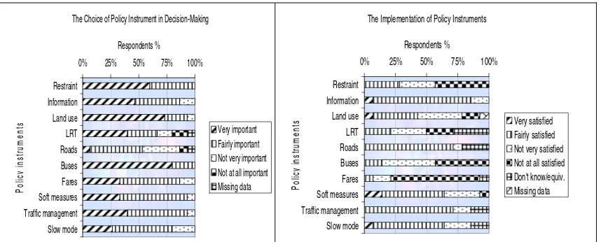
The most useful answers (apart from the individual text box answers) came from the importance and satisfaction questions about the different types of policy instruments and enabling factors.

Figure 1 summarises the importance and satisfaction given to modelling certain types of policy instruments. In general Light Rapid Transit (LRT), land use measures, road infrastructure, traffic restraint and improvements to bus services were seen to be most important while slow modes, information provision, traffic management and soft measures such as awareness campaigns were seen to be less important in terms of modelling.

[Insert Figure 1 around here]

In general most authorities were satisfied with the modelling of LRT, new road infrastructure and traffic management and to some extent land use measures. The level of satisfaction for other measures depended partly on the measure being considered and on the experience of models used by each local authority.

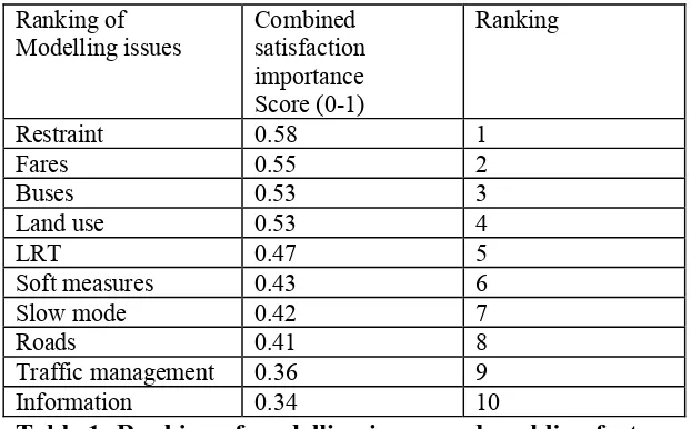
Table 1 combines these importance and satisfaction scores from each authority, normalising the mean importance and taking the product with the mean satisfaction score (see DISTILLATE (2005)). The scores give the following ranking of barriers by instrument type. A higher score implies that the instrument type is both important and has most room for improvement.

[Insert Table 1 around here]

From the above ranking and more detailed analysis of the questionnaires it was decided that the research should look at the following modelling themes :-

1. Demand restraint measures (e.g. parking charges/capacity, road user charging) 2. Public Transport improvements (quality bus corridors, capacity, bus priorities) 3. Land use measures (development controls)

4. Soft measures (attitudinal, awareness campaigns)

5. Slow modes and small scheme impacts (cycling and walking strategies) and more general issues

6. Data issues 7. Model use

(6)

identified from the above analysis.

3. The MARS model

MARS is a dynamic Land Use and Transport Integrated (LUTI) model. The basic underlying hypothesis of MARS is that settlements and activities within them are self organizing systems. Therefore MARS is based on the principles of systems dynamics (Sterman (2000)) and synergetics (Haken (1983)). The development of MARS started some 10 years ago partly funded by a series of EU-research projects (OPTIMA, FATIMA, PROSPECTS, SPARKLE). To date MARS has been applied to seven European cities (Edinburgh - UK, Helsinki - FIN, Leeds - UK, Madrid -ESP, Oslo - NOR, Stockholm – S, and Vienna – A) and 3 Asian cities (Chiang Mai and Ubon Ratchathani in Thailand and Hanoi in Vietnam).

The present version of MARS is implemented in Vensim®, a System Dynamics programming environment. This environment was designed specifically for dynamic problems, and is therefore an ideal tool to model dynamic processes.

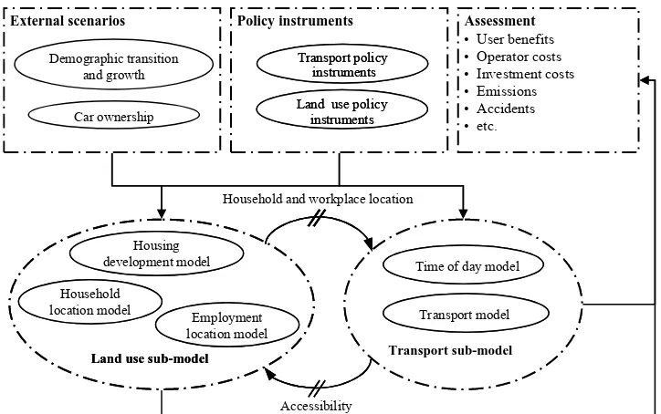
The MARS model includes a transport model which simulates the travel behaviour of the population related to their housing and workplace location, a housing development model, a household location choice model, a workplace development model, a workplace location choice model, as well as a fuel consumption and emission model. All these models are interconnected with each other and the major interrelations are shown in Figure 2. The sub-models are run iteratively over a 30 year time period. They are on the one hand linked by accessibility as output of the transport model and input into the land use model and on the other hand by the population and workplace distribution as output of the land use model and input into the transport model. The next section describes the main cause effect relations in a qualitative way. A comprehensive description of MARS can be found in Pfaffenbichler (2003).

Main cause effect relations

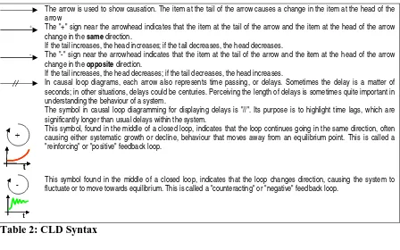
This section uses the Causal Loop Diagram (CLD) technique to explain one of the core sub-models of MARS namely the transport model.

Excursus: CLD method

The syntax of the CLD-method is very simple - there exist just arrows and the signs "+" and "-". But it is crucial to understand the meaning of "+" and "-".

The following table explains the used symbols:

[Insert Table 2 here]

Figure 3 shows the CLD for the factors which affect the number of commute trips taken by car from one zone to another. From

(7)

B3 show the impact on fuel costs, in our urban case as speeds increase fuel consumption is decreased – again we have a balancing feedback.

Loop B4 represents the effect of congestion on other modes and is actually a reinforcing loop – as trips by car increase, speeds by car and public transport decrease which increases costs by other modes and all other things equal would lead to a further increase in attractiveness by car. The other elements in

Figure 3 show the key drivers of attractiveness by car for commuting. These include car availability and attractiveness of the zone relative to others which is driven by the number of workplaces and population. The employed population drives the total number of commute trips and within MARS the total time spent commuting influences the time left for other non-commute trips. Similar CLDs could be drawn for other modes and for non-commute trips as MARS works on a self-replicating principle applying the same gravity approach to all sub-models.

It is this simple causal loop structure and user friendly software environment which helps improve the transparency of the modelling approaches used. The next section uses the CLD with the actual variables as input within the model to describe how the model was adapted to take into account bus quality and over-crowding factors.

[Insert figure 3 around here]

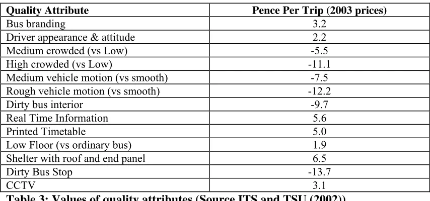
4. Quality bus factors and over-crowding

ITS reviewed the evidence on willingness to pay for attributes of bus quality and over-crowding (ITS & TSU, 2002) under the four general headings of

• Information Provision;

• Vehicle Type;

• Service Quality; and

• Passenger Infrastructure.

Table 3 summarises the values in pence per trip. It should be noted that care is needed when aggregating the value of several quality dimensions. We recommend that a package of quality measures should be valued at no more than 20 pence per trip for non-London trips. This stems from work carried out by ITS & TSU (2001) which, based their findings on the ‘package effect’ found by SDG in an earlier study (1996).

To implement a quality bus corridor in MARS a new policy variable was added where all quality factors could be incorporated into one input to the model. This user defined quality enhancement would then affect the absolute cost of bus/rail trips for the selected corridors. It is down to the user to define which of the measures are implemented from the above table. Thus one policy lever which can increase and decrease quality of service (with a maximum suggested benefit of 20 pence per trip) was created. The following describes the initial implementation in the Edinburgh model and results from implementing a +/- 20 pence per trip change in quality.

(8)

platform. This figure also shows where the over-crowding cost is introduced (discussed later).

[Insert figure 4 here]

The changes in quality were input in Euro-cents with range +/-30 cents which is approximately +/- 20 pence. The effect is the same as if a fare change were made to all OD pairs in absolute rather than percentage terms – without of course affecting the fare revenue directly.

The cost terms are translated from euros per trip to minutes per trip in the same way as are fares, namely :-

i PT ij PT ij Inc c Z . α

= Source. Eqn 4.20 from Pfaffenbichler (2003)

Where

PT ij

Z is the impedance from money costs of travelling from i to j by public transport

(minutes)

PT ij

c cost of public transport trip from i to j (€/trip)

is a factor of value of time; source Walther et al (1997) p19. Inci household income in zone i (€/minute)

Impact tests for quality factors

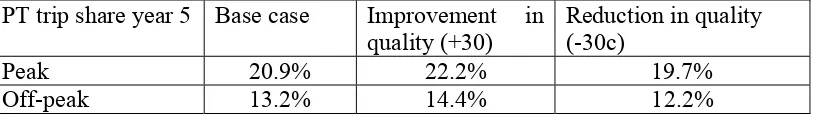
Two tests were conducted, one with a bus quality improvement worth +30 cents and one with quality decreasing by 30 cents worth (reflecting poor maintenance of bus stops and rough vehicle motion for example).

Both of these tests were compared against the base case in year 5 when the changes are assumed to take place. The share of PT trips in the peak and off-peak were output as follows :-

The changes in patronage are around +/-6% in the peak and +/-9% in the off-peak for the whole study area. The change in patronage obviously varies by OD pair and for those within the urban area the range was typically higher than average with some increasing by as much as 14%, while long distance routes had much lower increases of around 2%. These results are in line with evidence from TRL (2004) who found increases in patronage on quality bus corridors, where no journey time enhancements (bus lanes or traffic signal priorities) had been incorporated (e.g. effect of low floor bus & better marketing), of between +2% to +10%.

Over-crowding

(9)

The second approach is to add a discomfort factor to the in-vehicle time again this factor varies with occupancy level to represent discomfort. Both methods were implemented in MARS and were found to give similar answers. Given the lack of evidence on the form of the discomfort factor for the second approach the results presented here relate to the cost per trip approach.

Impact tests for over-crowding

The occupancy level in the peak was assumed to be 70% for these simple tests in year 0. This inclusion of medium over-crowding costs in year 0 for all peak services adds a small cost per trip and this has a small impact on initial mode splits. As public Transport demand is declining over the forecast period the over-crowding model has no impact on the do-nothing scenario. In order to test the impact of the crowding model we had to engineer a case where patronage increases so that the occupancy increases from 70% to more than 80%. This was achieved by reducing fares by 50%.

The following table shows the share of PT trips in the peak for a 50% fare reduction with and without the crowding factors.

As expected the increased crowding factors result in a slightly lower share of PT trips. These results are in line with the quality bus factor changes in patronage. This simple cost per trip approach to the modelling of over-crowding gives a reliable method of incorporating the effects without upsetting the mode choice process. Further research is planned whereby capacity of the route is modelled – representing the case where some users have to wait for the next bus. Current UK advice (DfT (2006), Webtag Unit 3.11.2) on this is that this type of approach may cause convergence problems within PT assignment and mode choice modelling, but we do not expect such problems with our dynamic modelling approach.

5. Introducing the Heavy Rail mode

One of the weaknesses identified with the MARS model was the fact that public transport in an urban area was aggregated into one representative mode – although the proportion of services which were separated from car traffic could be taken into account. This section describes the implementation and testing of the introduction of a fourth mode, heavy rail within the urban centre of Leeds. Figure 5 shows the study area for the Leeds model with the stations to be modelled.

The geographical scope of the Leeds MARS case study covers the 33 wards of Leeds which is an area of about 560 km² (Figure 5). The time horizon of the case study is 2031. MARS calculates the welfare function for each year up to the time horizon.

[Insert Figure 5 here]

MARS models the mode choice between public transport, private car and slow modes via the concept of friction factors. The following describes in detail the development of the friction factor related to public transport.

A trip with the mode public transport consists of four different parts:

(10)

• Travelling from the public transport stop to the destination

• Changing time

• Walking from the public transport stop to the destination

Each of these parts is perceived and valued differently by the public transport users. The different subjective valuation factors in Equation 1 reflect this fact.

(

)

PT

ij w PT Jj w PT Jj ch PT IJ ch PT IJ dr PT IJ wt PT I wt PT I w PT iI w PT iI PT ij PT

ij c t SV t SV t t SV t SV Z

t

f , = , * , + , * , +

∑

, +

∑

, * , + , * , +

Equation 1: Friction factor public transport (Walther et al., 1997) p. 20 ff

tPT,wiI...Walking time from source i to public transport stop I (min)

SVPT,wiI...Subjective valuation factor walking time from source to public transport stop

tPT,wtI...Waiting time at public transport stop I (min)

SVPT,wtI...Subjective valuation factor waiting time at public transport stop

tPT,drIJ...Total in-vehicle time from PT stop I to PT stop J (min)

tPT,chIJ...Total changing time from PT stop I to PT stop J (min)

SVPT,chIJ...Subjective valuation factor changing time

tPT,wJj...Walking time from public transport stop J to destination j (min)

SVPT,wJj...Subjective valuation factor walking time from public transport stop to destination ZPTij...Impedance from costs travelling from i to j by public transport (min)

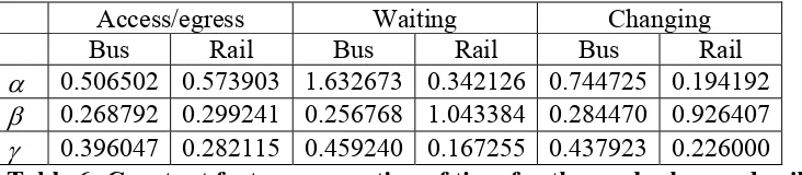
(Walther et al., 1997) defines separate friction factors for the public transport modes bus, tramway and underground/light rail. MARS makes a distinction whether public transport is separated from individual road traffic or not. The subjective valuation factors used in MARS have the principal form as shown in Equation 2. The values for the parameters can be found in (Walther et al., 1997) p. 21-23.

k PT ij t k PT ij e

SV , =α+β* γ* ,

Equation 2: Subjective valuation factor for the different parts of a public transport journey

SVPT,kij...Subjective valuation factor for part k of public transport journey from i to j

α, β,γ...Constant factors

tPT,kij...Time for part k of a public transport journey from i to j (min)

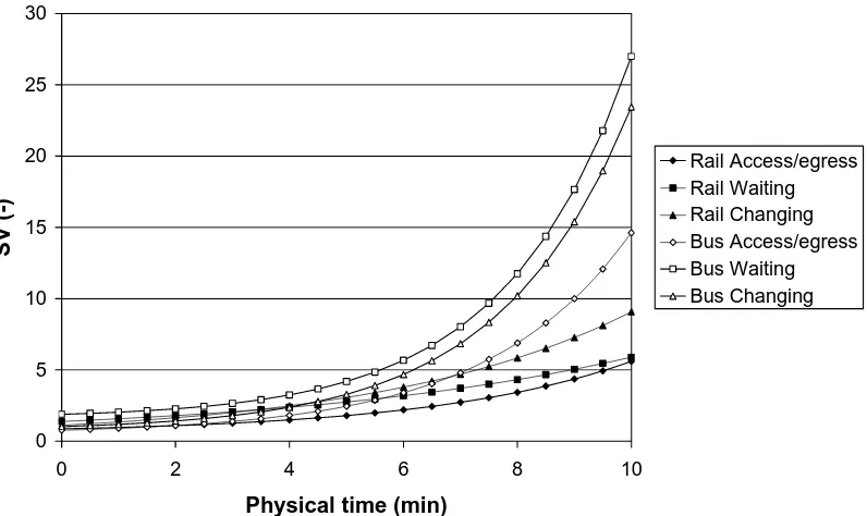
Figure 6 shows the subjective overestimation of access/egress, waiting and changing time in relation to physical time for the public transport modes bus and rail.

[Insert table 6 here]

The following friction factor for public transport money costs is used in MARS (Walther et al., 1997) p. 19:

i PT ij PT ij Inc c Z * α =

Equation 3: Friction factor from public transport costs

cPTij...Costs for a public transport trip from i to j (€/trip)

α...Factor for value of time; 0.17 Source: (Walther et al., 1997) p. 19

(11)

To implement a the heavy rail mode data on headways, distance, fares and speeds between the urban stations and Leeds central for the peak and off-peak were taken from a more detailed model developed by ITS for JMP(2004). The only data which needed to be estimated further was the average access and egress times to and from stations for the relevant zones. A map of Leeds was used to estimate the access and egress distances. The built up area was subdivided into segments and the distances between their centroids and the next railway station were measured. The access and egress distance was calculated as the weighted average of these distances. The surface of the built up areas was used as weight because there was no detailed information available about the population of the built up areas.

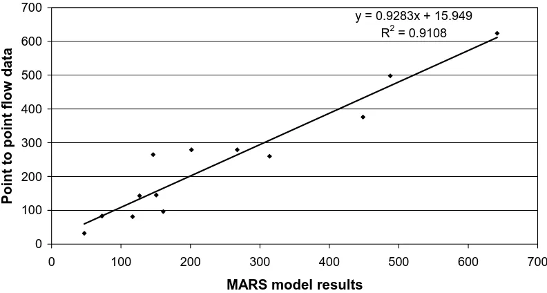
With this data the Heavy Rail mode was implemented with subjective values taken from Walther et al (1997) for commuter rail. The results of implementing heavy rail in this way were compared against point to point flow data as follows :-

[Insert Figures 7 and 8 around here]

Figure 7 shows the model fit between the forecast model flows and the point to point data for the peak. The model gave a reasonable fit with an R2=0.91. Figure 8 shows the assigned flows along the lines for those stations within the urban area modelled. Although the heavy rail only accounts for 0.6% of the total trips in the peak the rail share along the corridors was seen to be 6.8%. Further tests with the rail model will be made to investigate how other policy instruments such as road pricing affect the rail movements.

6. Conclusions and future research

This paper has demonstrated how MARS has been adapted to quantify the impacts of soft (qualitative) measures such as bus branding, quality of ride, driver appearance, overcrowding etc. The changes needed have been incorporated within the simple causal loop diagram so that any decision-maker can see how the factors have been introduced. The results of applying the simple cost per trip based approach to improved bus quality resulted in changes in patronage which were in line with the latest evidence.

Two possible models for incorporating over-crowding were considered, one based on a simple cost of medium/high over-crowding per trip and the other on a discomfort factor applied to in-vehicle time. Following UK advice the simple approach was adopted but future tests will be conducted with more complex representation of the capacity of bus corridors.

Finally we demonstrated how the basic MARS model could be adapted to give more detailed results for heavy rail corridors within an urban area such as Leeds. Further policy tests will be conducted to investigate the potential for interaction between demand restraint policies and heavy rail provision.

(12)

was recognised to be very important and will be tackled by the introduction of a so called population cohort model. This model enables us to simulate the development of the structure of the population over time more realistically and to test new policies which depend on age, for example the recent policy to increase the retirement age to 68 which will obviously impact on the number of commute trips.

Decision makers and planners also wish to find optimal policy combinations at the strategic level. For this we intend to make use of the Vensim® optimisation routines provided within its simulation environment. We aim within the DISTILLATE project to develop the front-end so that local authority planners can use these facilities to optimise policy combinations themselves against a pre-defined objective or set of indicators via a cost-benefit or multi-criteria analysis.

(13)

References

Department for Transport (2006) “Road Traffic and Public Transport Assignment Modelling”. WebTag Unit 3.11.2.

http://www.webtag.org.uk/webdocuments/3_Expert/11_Specifications/3.11.2.htm

DISTILLATE (2005) : Project A Deliverable A1: Findings of the 'Phase 1' Survey on the Barriers to the Delivery of Sustainable Transport Solutions (February 2005)

http://www.distillate.ac.uk/Reports.html

Institute for Transport Studies (University of Leeds) and Transport Studies Unit (University of Oxford) (2002) “Quality Bus Partnership and Market Structure – A Review of Evidence”. Report to the DETR.

Haken, H. (1983). Advanced Synergetics - Instability Hierarchies of Self-Organizing Systems and Devices, Springer-Verlag.

JMP Consultants (2004) “Rail in the City Regions”. Report Prepared for PTEG. Martens M, Pedler A and Paulley N (2002). The assessment of integrated land use and transport planning strategies. European Transport Conference. Cambridge, 9-11 September 2002

May, A.D. (2004) : DISTILLATE Inception Report. July 2004.

http://www.distillate.ac.uk/Reports.html

Pfaffenbichler, P. (2003). The strategic, dynamic and integrated urban land use and transport model MARS (Metropolitan Activity Relocation Simulator) - Development, testing and

application, Beiträge zu einer ökologisch und sozial verträglichen Verkehrsplanung Nr. 1/2003, Vienna University of Technology, Vienna.

Shepherd, S.P., Timms, P.M, May A.D. (2006) Modelling Requirements For Local Transport Plans: An Assessment Of English Experience. Transport Policy Volume 13 Issue 4 pp 307-317 July 2006.

Simmonds D C, May A D and Bates J J (2001). A new look at multimodal modelling. Proc 18th European Transport Conference, London: PTRC

Steer Davies Gleave (1996) “Bus Passenger Preferences. For London Transport Buses.” London: SDG.

Sterman, J. D. (2000). Business Dynamics - Systems Thinking and Modeling for a Complex World, McGraw-Hill Higher Education.

TRL (2004). Demand for Public Transport. TRL Report 593. (2004).

(14)

Ranking of Modelling issues

Combined satisfaction importance Score (0-1)

Ranking

Restraint 0.58 1

Fares 0.55 2 Buses 0.53 3

Land use 0.53 4

LRT 0.47 5

Soft measures 0.43 6

Slow mode 0.42 7

Roads 0.41 8

Traffic management 0.36 9

[image:14.595.83.394.98.291.2]

Information 0.34 10

Table 1: Ranking of modelling issues and enabling factors.

(15)

The arrow is used to show causation. The item at the tail of the arrow causes a change in the item at the head of the arrow

The "+" sign near the arrowhead indicates that the item at the tail of the arrow and the item at the head of the arrow change in the same direction.

If the tail increases, the head increases; if the tail decreases, the head decreases.

+

The "-" sign near the arrowhead indicates that the item at the tail of the arrow and the item at the head of the arrow change in the opposite direction.

If the tail increases, the head decreases; if the tail decreases, the head increases.

-

In causal loop diagrams, each arrow also represents time passing, or delays. Sometimes the delay is a matter of seconds; in other situations, delays could be centuries. Perceiving the length of delays is sometimes quite important in understanding the behaviour of a system.

The symbol in causal loop diagramming for displaying delays is "//". Its purpose is to highlight time lags, which are significantly longer than usual delays within the system.

+

tt

This symbol, found in the middle of a closed loop, indicates that the loop continues going in the same direction, often causing either systematic growth or decline, behaviour that moves away from an equilibrium point. This is called a "reinforcing" or "positive" feedback loop.

This symbol found in the middle of a closed loop, indicates that the loop changes direction, causing the system to fluctuate or to move towards equilibrium. This is called a "counteracting" or "negative" feedback loop.

-

[image:15.595.90.538.82.362.2]

tt

(16)

Quality Attribute Pence Per Trip (2003 prices)

Bus branding 3.2

Driver appearance & attitude 2.2

Medium crowded (vs Low) -5.5

High crowded (vs Low) -11.1

Medium vehicle motion (vs smooth) -7.5

Rough vehicle motion (vs smooth) -12.2

Dirty bus interior -9.7

Real Time Information 5.6

Printed Timetable 5.0

Low Floor (vs ordinary bus) 1.9

Shelter with roof and end panel 6.5

Dirty Bus Stop -13.7

[image:16.595.84.511.83.283.2]

CCTV 3.1

(17)

PT trip share year 5 Base case Improvement in quality (+30)

Reduction in quality (-30c)

Peak 20.9% 22.2% 19.7%

[image:17.595.89.497.86.146.2]

Off-peak 13.2% 14.4% 12.2%

(18)

Do-nothing Fare -50% no crowding

Fare -50% with crowding PT share peak year 5 20.9% 25.5% 24.9%

(19)

Access/egress Waiting Changing Bus Rail Bus Rail Bus Rail

α 0.506502 0.573903 1.632673 0.342126 0.744725 0.194192

β 0.268792 0.299241 0.256768 1.043384 0.284470 0.926407

[image:19.595.87.453.85.165.2]

γ 0.396047 0.282115 0.459240 0.167255 0.437923 0.226000

(20)

The Choice of Policy Instrument in Decision-Making

0% 25% 50% 75% 100%

Restraint Information Land use LRT Roads Buses Fares Soft measures Traffic management Slow mode P olic y in st ru m en ts Respondents % Very important Fairly important Not very important Not at all important Missing data

The Implementation of Policy Instruments

0% 25% 50% 75% 100%

[image:20.595.85.514.84.257.2]

Restraint Information Land use LRT Roads Buses Fares Soft measures Traffic management Slow mode P olic y i ns tr um ent s Respondents % Very satisfied Fairly satisfied Not very satisfied Not at all satisfied Don't know/equiv. Missing data

(21)

Demographic transition and growth Car ownership External scenarios Transport policy instruments Transport policy instruments Transport policy instruments Policy instruments

Land use policy instruments Land use policy

instruments Land use policy

instruments

Time of day model

Transport model

Transport sub-model

Time of day model Time of day model

Transport model Transport model

Transport sub-model Assessment

• User benefits • Operator costs • Investment costs • Emissions • Accidents • etc. Housing development model Household location model

Land use sub-model

Employment location model Housing development model Household location model

Land use sub-model

Employment location model

Household and workplace location

[image:21.595.117.479.68.295.2]

Accessibility

(22)

Commute trips by car

Speed by car Attractiveness by car + - B1-Commute cost by car -Attraction + Workplaces Population + + Fuel cost + - B3-Total commute trips Employed population + +

Car availability Car ownership

+

Commute cost other modes

+

Time in car commute -Parking search time + + Attractiveness of

other zones

-Total commute time + Time per commute trip + +

Time for other trips

-Time per commute trip by other modes

-+

B2-+

B4+