Model structure selection in powertrain calibration and control

(1)

Calibration and Control

Thesis submitted in accordance with the requirements of the

University

of

Liverpool

for the

Degree of Doctor in Philosophy

by

Zongyan Li

(2)

Statement of Originality

This thesis is submitted for the degree of Doctor in Philosophy in the Faculty of Engi-neering at the University of Liverpool. The research project reported herein was carried out, unless otherwise stated, by the author in the Department of Engineering at the University of Liverpool between 1/11/2008 and 31/10/2012.

No part of this thesis has been submitted in support of an application for a degree or qualification of this or any other University or educational establishment. However, some parts of this thesis have been published, or submitted for publication, in the following papers:

• Li Z. and Shenton A.T. (2010) Nonlinear Model Structure Identification of Engine

Torque and Air/Fuel Ratio. 6th IFAC Symposium Advances in Automotive Control. IFAC, Munich pp 1-6

• Li Z. and Shenton A.T. (2010) Structure Selection for Identified Multi-Model Dynam-ic Fuel Maps. 10th International Symposium on Advanced VehDynam-icle Control. AVEC, Loughborough pp 1-6

• Shenton A.T. and Li Z. (2012) Multi-Modelling of Torque and Air/Fuel Ratio Based

on Engine Operating Regions. 15th IFAC Workshop on Control Applications of Opti-mization, Volume.15, Part 1. IFAC, Rimini

• Li Z. and Shenton A.T. (2012) I.C. Engine Inverse Dynamic Multi-Model Identification. In Proceeding of Powertrain Modelling and Control Conference, Paper 16, Bradford

Zongyan Li

20th October 2012

(3)

Abstract

This thesis develops and investigates the application of novel identification and structure

identification techniques for I.C. engine systems. The legislated demand for reduced

vehi-cle fuel consumption and emissions indicates that improved model-based dynamical engine

calibration and control methods are required in place of the existing static set-point based

mapping methods currently used in industry. The choice of structure of any dynamical engine

model has significant consequences for the accuracy and the calibration/optimization time of

engine systems. This thesis primarily addresses the issue of this structure selection.

Linear models are well understood and relatively easy to implement however the modern

I.C. engine is a highly nonlinear system which restricts the use of linear structures. Further

the newer technologies required to achieve demanding fuel consumption and emission targets

are increasingly more complex and nonlinear. The selection of appropriate nonlinear model

regressor terms presents a combinatorial explosion problem which must be solved for accurate

engine system modelling. In this thesis, two systematic nonlinear model structure selection

techniques, namely stepwise regression with F-statistics and orthogonal least squares method

with error reduction ratio, are accordingly investigated. SISO algebraic NARMAX engine

models are then established in simulation studies with these methods and demonstrate the

effectiveness of the approach.

The thesis also investigates the development and application of multi-modelling

tech-niques and the expansion of the model structure selection techtech-niques to the identification of

the local models terms within the multi-model structures for the engine. Based on the

en-gine operating regions, novel multi-model networks can be established and several alternative

multi-modelling techniques, such as LOLIMOT, Neural Network, Gaussian and log-sigmoid

function weighted multi-models, for the multi-model engine system identification are explored

and compared. An experimental validation of the methods is given by a black box

(4)

cation of SISO engine models which are developed purely from the experimental engine test

data sets. The results demonstrate that the multi-model structure selection techniques can

be successfully applied on the engine systems, and that the multi-modelling techniques give

good model accuracy and that good modelling efficiency can also be achieved.

The outcome is a set of techniques for the efficient development of accurate nonlinear

black-box models which can be acquired from experimental dynamometer test-bed data which

should assist in the dynamic control of future advanced technology engine systems.

(5)

I am very grateful to my supervisor Dr Tom Shenton. His guidance and support were

indispensable and much appreciated in the completion of this work. I also want to thank my

supervisor Prof. Huajiang Ouyang for his timely and valuable advice while I was progressing

the PhD. I would like to thank Dr Ahmed Abass, Dr Paul Dickinson, Ke Fang, Ming-yen

Chen and Kamil for kindly offering their valuable suggestions and assistance. I would like to

thank my parents for their inspiration and selfless financial support for my study in the UK.

Finally, my gratitude goes to my wife, Qin Chen, for her love and patience.

(6)

List of Figures

2.1 The Flow Chart of System Identification . . . 8

2.2 Black-box and White-box Models comparison . . . 12

2.3 Linear black-box model classes . . . 14

2.4 The identified dynamical model with a series of unit tapped delays . . . 15

3.1 A schematic structure of the engine connecting with dynamometer . . . 19

3.2 The key control devices for the engine test . . . 20

3.3 Variable Camshaft Timing scheme . . . 22

3.4 Inputs and Outputs of the VCT Engine . . . 24

3.5 VCT Engine Simulation Model in Simulink . . . 25

3.6 Throttle and Manifold Simulation Model . . . 25

3.7 VCT Engine Torque Model . . . 26

3.8 Inputs and Outputs of the Diesel Engine with VGT mechanism . . . 27

3.9 WAVE model developed for GTDI engine . . . 29

4.1 The data used for the SISO model identification . . . 39

4.2 The data used for the SISO model validation . . . 39

4.3 Coherence estimate via Welch’s method . . . 41

4.4 Order selection analysis . . . 41

4.5 The ARX model validation . . . 43

4.6 The investigation of the models obtained by different algorithms . . . 43

4.7 The structure of NARX model estimator . . . 44

4.8 The NARX model validation in Simulink . . . 46

4.9 The NARX model residual . . . 47

(10)

5.1 Pool of Regressors . . . 51

5.2 Structure Selection Flow Chart . . . 51

5.3 Stepwise Regression with F-statistics . . . 54

5.4 Orthogonal Least Squares with ERR detection . . . 59

5.5 Input Channels . . . 64

5.6 Prediction of torque using correlation criteria and ERR criteria . . . 65

5.7 Prediction of air/fuel ratio using correlation criteria and ERR criteria . . . . 65

6.1 The taxonomy of multi-models . . . 70

6.2 The generic multi-model structure . . . 71

6.3 Gaussian bell curves . . . 74

6.4 Log-sigmoid curves . . . 75

6.5 ARX/NARX model as block diagram with tapped time delays . . . 76

6.6 Relations between model fitness and regressor number . . . 78

6.7 Relations between model fitness and multiplication number . . . 78

6.8 Log-Sigmoid weighting function . . . 80

6.9 The infrastructure of the neural network model . . . 81

6.10 The test data of engine speed . . . 81

6.11 Torque Estimation using Nonlinear Multi-Affine Model . . . 82

6.12 Torque Estimation using Neural Network Model . . . 82

6.13 Air/fuel ratio Estimation using Nonlinear Multi-Affine Model . . . 82

6.14 Air/fuel ratio estimation using neural network model . . . 83

6.15 2D partitioning of LOLIMOT algorithm . . . 85

6.16 Flow chart of the LOLIMOT algorithm . . . 86

6.17 The LOLIMOT structure as a neural network . . . 86

6.18 Test data sets for LOLIMOT identification . . . 87

6.19 Data partitioning process (N: Engine speed L: Lambda) . . . 88

6.20 Weighting function curves . . . 89

6.21 Validation of the LOLIMOT model . . . 89

6.22 Local model number analysis . . . 90

7.1 Input channels for multi-model identification . . . 95

(11)

7.3 2D Scheduling for Torque and Air/Fuel Ratio . . . 97

7.4 Estimated vs Measured Air/Fuel Ratio by Error Reduction Ratio Analysis . . 98

7.5 Estimated vs Measured Torque Output by F-statistic Analysis . . . 99

7.6 R2 vs Multi-model Number for Air/Fuel Ratio Estimation . . . 99

7.7 Inverse MISO multi-model structure . . . 100

7.8 WAVE-RT engine test setup for inverse MISO multi-model . . . 101

7.9 Data channels of the inverse multi-model . . . 102

7.10 Data partitioning tree . . . 102

7.11 2D data partitioning with MAP and RPM . . . 103

7.12 The validation result of Inverse multi-model for spark advance (SA) . . . 103

7.13 The validation result of Inverse multi-model for throttle angle (THR) . . . . 103

7.14 A open-loop simulation of the inverse control . . . 104

8.1 The boundaries for the curve of the weighting function . . . 109

(12)

List of Tables

5.1 Input and Output Channels . . . 63

5.2 Stepwise Regression Using F-statistics (Reg: Regressor number) . . . 63

5.3 Regressers and Parameters in the Torque Model . . . 67

5.4 Regressers and parameters in the Air/Fuel Ratio Model . . . 68

5.5 Model Prediction Quality . . . 68

6.1 CORR and ERR Structure Selection Process at 1750rpm . . . 79

6.2 Local Linear Models for Torque(y1)and Air/Fuel Ratio(y2) . . . 92

7.1 Input and Output Channels . . . 94

7.2 Model Prediction Quality . . . 98

(13)

ABV Air-Bleed Valve

ACF Auto-Correlation Function

AFR Air-Fuel Ratio

AIC Akaikes Information Criterion

PRBS Modulated Pseudo-Random Binary Sequence

ATDC After Top Dead Centre

ARMAX AutoRegressive Moving Average with eXogeneous inputs

ARX AutoRegressive with eXogeneous inputs

BDC Bottom Dead Centre

BIC Bayesian Information Criterion

BJ Box-Jenkins

BTDC Before Top Dead Centre

DoE Design of Experiment

ECU Engine Control Unit

EGR Exhaust Gas Recirculation

EMS Engine Management System

FPE Final Prediction Error

FPW Fuel Pulse Width

FIR Finite Impulse Response

GDI Gasoline Direct Injection

GTDI Gasoline Turbocharged Direct Injection

HEGO Heated Exhaust Gas Oxygen

IC Internal Combustion

INJ Injected fuel mass

MAP Manifold Air Pressure

MIMO Multiple-Input-Multiple-Output

MISO Multiple-Input-Single-Output

MLE Maximum Likelihood Method

MSE Mean Squared Error

NARX Non-linear AutoRegressive Moving Average

NN Neural Network

(14)

OE Output Error

OLS Ordinary Least Square

PEM Prediction Error Method

PFI Port Fuel Injection

PRBS Pseudo Random Binary Sequence

PS Pattern Search

PSD Power Spectral Density

RBS Random Binary Signal

RPM Revolutions Per Minute

RT Real Time

SA Spark Advance

SAN Simulated ANnealling

SEM Simulation Error Method

SI Spark Ignition

SISO Single-Input-Single-Output

SQP Sequential Quadratic Programming

TDC Top Dead Centre

THR Throttle Angle

TRR Trust Region Reflective

TWC Three Way Catalyst

UDRN Uniformly Distributed Random Number

UEGO Universal Exhaust Gas Oxygen

VGT Variable Geometry Turbocharger

(15)

Introduction

The modern automotive I.C. engine system requires accurate and multi-dimensional

calibra-tion in order to meet increasingly strict emission and fuel consumpcalibra-tion regulacalibra-tions. The trend

of engine development is to the use of additional actuators, sensors and of more complex

tech-nologies with more prevalent transient dynamics. As a result, the number adjustable variables

in the engine operating space are increasing significantly which means that even more data

samples clustered across the larger operating space are needed to determine sufficient

informa-tion for statistically reliable engine calibrainforma-tion. Because the number of required data points

and corresponding optimisation effort increases exponentially with the number of adjustable

variables, this phenomena is known as ’curse of dimensionality’ [1]. Notwithstanding the

sig-nificant improvements brought by advanced numerical optimisation and design-of-experiment

(DoE) methods, due to the ’curse of dimensionality’ the cost of experimental based engine

tests to support the conventional static calibration procedures is becoming exponentially

time-consuming and costly. One potential way of addressing this issue is to capture

experi-mental data in a dynamic model during non-steady-state testing [2]. An additional advantage

of a dynamic modelling is that it may allow control of the engine dynamics which are likely to

become of increasing significance in forthcoming legislated drive cycles which have significant

engine transients and tightened emissions [3].

To capture the nonlinear dynamical behaviour of the advanced I.C. engine system

(16)

CHAPTER 1. INTRODUCTION 2

ever requires an efficient and reliable way to determine model type and subsequently model

parameters in the system-identification. Dynamic black-box identified polynomial models

have been widely considered by researchers for engine management system (EMS) mappings

instead of the current steady-state static pseudo-dynamic methods [4]. Hybrid structured

multi-models have been reported as being able to provide a capability to represent complex

nonlinear characteristics with the desired simple structure, however there are many choices

for the multi-model structure, including nonlinear terms, partition size, weighting choice,

lin-ear vs nonlinlin-ear etc. [5]. Such dynamic maps have the potential to improve emissions and fuel

consumption in transient operations for reduced computational time and ease of

implemen-tation including comprehension and calibration. Accordingly, structure selection methods

are required to choose the simplest effective models. Structure identification techniques to

determine the optimal structures of black-box models are the principal subject of this thesis.

1.1 Systems identification of SISO and MIMO models

The study of Single-Input-Single-Output (SISO) systems offer a way to reveal the cause

and effect interconnection between two variables and it is the central concern of system

identification. For a newly designed system or a manufactured item, we would always ask the

question like how will all the inputs affect the system outputs or what uncertainties the system

has. SISO models can be used to relate variables of any component in the engine whether

it is a small part such as a spark plug or a larger mechanism namely a turbocharger. The

SISO models are generally identified based on input/output data and physical information

gathered from the system [6]. Three significant areas are required to be considered before

the identification:

• Prior knowledge about physical phenomena

The behavior of the systems is guided by a series of physical principles such as Newton’s

laws and energy conservative laws, therefore, some outputs of the system are fully

predictable according to the physical analysis. For example, in an engine intake system,

(17)

of the cross section. Engine speed can be derived from the brake torque and crankshaft

inertia.

• Observed data

The observed data is the key information source for a complex system because physical

analysis becomes unfeasible due to the curse of dimensionality. The input signal design

is a significant procedure to make sure the information contained in the data is rich

enough. Meanwhile, the measured data is used to compare with the model output and

thus validate the model quality. The observed data can be measured directly by the

sensors in the system or indirectly calculated by measured data.

• Accuracy requirement of the model

Most of the model structure determination process runs iteratively thus a stopping

criteria is necessary for the identification process. This means the identified models are

only acceptable when certain thresholds are satisfied. The model with high accuracy is

significant but complex model structures may cost a long time in training the data and

calculating the output. A balance must be found otherwise it would make the model

difficult to be implemented in the real-time control systems.

In this thesis, SISO identification and structure selection techniques and also

Multiple-Input-Single-Output (MISO) system identification are investigated. In a complex engine

system, the output is always affected by various inputs and their cross relations. The proposed

strategy for a MIMO identification problem is to convert the Multiple-Input-Multiple-Output

(MIMO) identification problem into a network of MISO models which can be solved separately

when the outputs of the system are relatively independent of each other. With proper data

acquisition interface, such as dSPACE A/D conversion module, the data can be captured

and processed when the target system is in operation. In this case, the time-domain MIMO

models can also be identified in real-time by recursive least-squares estimation [7].

1.2 Overview

This thesis investigates various model structure selection techniques. Novel SISO and MISO

(18)

CHAPTER 1. INTRODUCTION 4

identified and validated on both a real and virtual engine setups.

Following this introduction, Chapter 2 introduces the general procedures of system

i-dentification. Both the static and dynamic system properties are discussed. The white-box,

black-box and grey-box model categories are described, especially the linear and nonlinear

black-box models. The model-based engine calibration is discussed as well.

Chapter 3 shows the infrastructures of four different engine test beds used in studies in

this thesis and introduces the sensors and actuators mounted on them.

Chapter 4 gives a detailed study of the application of Least Squares algorithm in

deter-mining the parameters of dynamical polynomial models. A series of dynamical SISO engine

models including linear and nonlinear ABV-RPM model are established and validated.

Chapter 5 demonstrates two major model selection techniques: the stepwise regression

with F-statistic analysis and the orthogonal least squares with error reduction ratio analysis.

The ANOVA algorithm is also introduced in this chapter. The dynamic models constructed

with these techniques are currently limited to linear, square and cubic regressors terms but

can be readily extended if necessary. A novel MISO dynamical model is developed by

appli-cation of the model structure selection techniques.

Chapter 6 extends the scope of model structure selection to the multi-model

identifi-cation. A number of multi-model structures are investigated, namely the LOLIMOT, and

the Neural Network. The general procedure of multi-modelling is described in this chapter.

Several novel dynamical multi-models are developed for different types of engines.

Chapter 7 applies an multi-model identification process to produce a novel forward and

inverse multi-model. The WAVE-RT virtual engine is adopted as the experiment test bed.

The forward model gives accurate estimation of the engine torque and air/fuel ratio whilst the

(19)

identified inputs.

Chapter 8 reviews the main outcomes of this thesis and discusses the thesis contributions

together with the future possible developments of these efforts.

1.3 Contributions

The novel contributions of this thesis are as follows:

• SISO dynamical models were developed based on PFI gasoline engine in Chapter 4.

The model structure are found by Matlab identification toolbox and validated by the

measured data. The polynomial model structure was adopted, especially, the

least-squares technique is adopted to determine the parameters of the models. Finally, both

ARX and NARX models of the engine system has been obtained.

• MISO dynamical models for IC engine was developed using stepwise regression and

orthogonal least squares techniques in Chapter 5. At the same time the detailed steps

of the iterative structure selection procedure are presented.

• A LOLIMOT model and a log-sigmoid weighted multi-model was established for IC

engines. The optimal number of local models is analysed according the multi-modelling

results.

• An inverse multi-model has been identified on a state-of-the art virtual engine model. The inverse model has been implemented to track the engine outputs of torque and

(20)

Chapter 2

Background

2.1 Dynamical System Identification for IC Engine

2.1.1 Static and Dynamical Modeling

A model for a system describes part or all of its characteristics depending on its application.

If we define two time pointst1 and t2 with u(t1) =u(t2) as their corresponding inputs, for

the static model, the model outputs would turn out to be y(t1) = y(t2). The relationship

between inputs and outputs remained unchanged with time in a static system. However, in

a dynamical system, the relationship is constantly evolving with time. In other words, the

outputs of static system only depend on the current inputs, but the outputs of dynamical

system will be affected by both current and previous inputs along the time line. In detail,

some modeling and control strategies for dynamic systems has been researched in [8, 9, 10].

2.1.2 Dynamic Engine Identification

System identification is a fundamental problem in systems engineering applications. The

application of system identification overlaps the boundaries of engineering and physical

sci-ence. Many other fields of study, such as economics and medicine, can also benefit from the

employment of system identification technology. Generally, system identification is the

(21)

termination of a mathematical model for a system or a process by observing its input-output

relationships [11]. In another word, a specific mathematical model which is equivalent in

input-output behaviour to a physical system can be obtained by this technology.

As the foundation of system identification, the input and output data should be

col-lected in a pre-designed experiment. Initially, the engine system is monitored by a set of

sensors and actuators according to our a priori knowledge, then a mathematical model for

the engine is developed by using structure selection and parameter estimation algorithms.

The engine model should be capable of reproducing the dynamics of the system over different

operating regimes. An accurate identified engine model is significantly beneficial for engine

calibration and control purposes. A schematic flow chart of the identification process is given

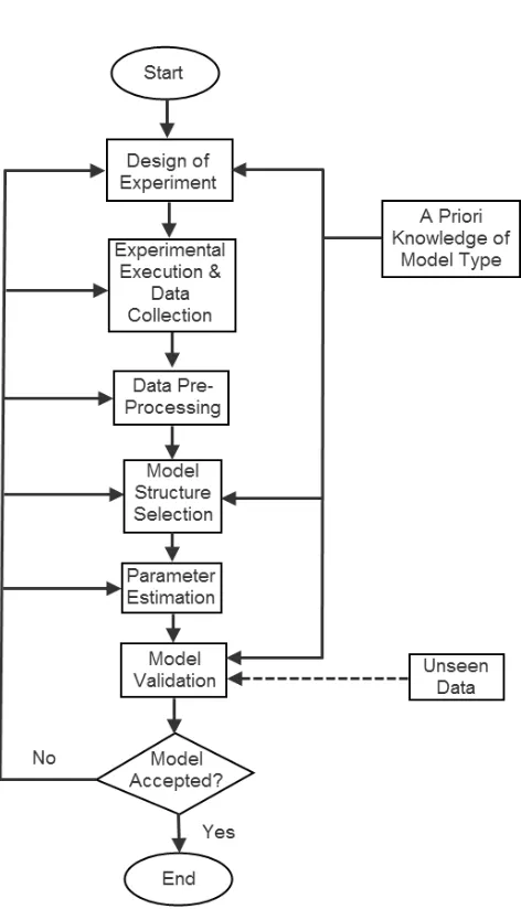
in Figure. 2.1 [12, 13, 14]

Design of Experiment

Dynamic system behaviour is represented by the current and past values of inputs and outputs

especially the transient response between the inputs and outputs. The experiment design

process applies clustering algorithm to locate a set of feasible operating points in order to

established dynamical model on a pre-defined working range with satisfying accuracy [15, 16].

To start an identification and control task, the input and output signals are to be

de-termined at the beginning. In the process of designing the experiment, a strategy of how

to efficiently and accurately acquire the information from the available experimental setup

should be established. In the case of engine test, the input and output signals are typically

transmitted into an A/D converter and processed in the computer. This means the resolution

and the sampling time of the sensor and actuator mounted on the engine must be

consid-ered in order to make sure the I/O data can be collected and managed in a sensible way.

Some prior knowledge of the system is vital because any experimental system has its

operat-ing limitations and experiment should always be conducted within the safe operatoperat-ing range.

Furthermore, the input and output signals need to be measurable within the experimental

budget. It is wise to avoid some parameters which are difficult to measure by indirectly

mea-suring related parameters. For instance, the throttle valve duty cycle is replaced by the Air

(22)

[image:22.595.214.450.205.617.2]

CHAPTER 2. BACKGROUND 8

(23)

instead of fuel injection mass. There are three major concerns in the design of the input

signals to be used for identification:

• Frequency Spectrum and Perturbation Time

The bandwidth of a dynamic system should be much wider than that of a static system.

Therefore, a proper input perturbation signal should be capable of exciting the system

across its bandwidth and revealing its nonlinearity as accurately as possible. In many

cases, step-shaped input signals, which change abruptly from one input value to another,

are preferred because they are equivalent to the superpositions of sinusoidal components

across an infinite number of frequencies. However, it is necessary to be aware that

instant change of the magnitude of input signal may result in damage to the test

equipment. The Pseudo Random Binary Sequence (PRBS) is another preferred option

in a digitally controlled experiment. The PRBS signal has the advantage of a wide

range of frequency content and a flat power spectrum density which is suitable for

dynamic identification. Other than the bandwidth of the PRBS signal which covers

a large spectrum between its lower frequency and upper frequency, the perturbation

time is also a deciding matter. The identified model of a dynamic system can only

be recognized as a good representation when the perturbation time is longer than the

delays of the system.

• Amplitude of the Signal

The amplitude of the signal does not pose any significant threat to the model accuracy

in linear identification applications because the gain of the system’s transfer function

is constant, in which case the output signal is proportional to the input. Therefore, the

PRBS signal with its two distinct levels is well accepted. For largely nonlinear systems,

the random walk signals which generated by uniformed random PRBS, a gain and an

integrator is believed to be a good choice. The variation of the signal amplitude of the

random walk signal aims to cover all the operating range of the nonlinear system and

capture the uncertainty within the nonlinear system.

• Sampling rate

The sampling rate refers to the time interval between the current and the subsequent

record of the signal generated by the sensors. The main constraint on achieving an

(24)

achieve the speed of sampling required. It has been recommended [14] that the sampling

rate to be 10 times that of the interested variable’s bandwidth. For best results, the

highest sampling rate is usually adopted in any engine test and the researcher will then

be able to decide the down-sampling strategy depending on the modeling requirements.

It is worth noting that the down-sampling can only be applied after any sort of digital

anti-aliasing filtering [17]. At the same time, the test input signal designer should also

keep the input signal rate lower than that of the sampling rate.

Data Processing

Due to various requirements of an identification algorithm, the experimental data collected

from an engine test should be adjusted into suitable form. The oversampling of the recorded

data, the associated sensors noise and the switching of electronic noise should all be considered

as factors in the data processing.

1. Offsets Removal and Data Detrending

In a general engine test system, the sensors for physical measurement could lead to

bias or offset. To remove the offsets such as those existing in absolute pressure or

tem-perature measurement from the data greatly improves the quality of the identification

process [18]. Therefore, the mean value of the data is eliminated from the raw data

samples respectively. Alternatively, the offset term can be deducted from the I/O

sig-nal in the identification process. Offsets can be revealed in the raw data or detected

in general trends like linear drifts or seasonal trends, and thus the best fitted trend is

subtracted from the I/O data in order to cancel these trends [17]. Usually, the sampling

rate is taken as higher than necessary in order to improve the optimizing result with the

amount of increase in rate based on the specific accuracy requirements. Since a system

with high order dynamics can have both fast and slow modes such a system may need

to be measured at high rate over a longer time requiring many more data samples than

for a system with low order dynamics. Further a high order system may require a much

faster sampling rate to capture its transient nonlinear behaviour, whereas a lower order

model containing a similar nonlinearity can be obtained with a much reduced sampling

(25)

2. Elimination of Outlier Points

Outlier points are the non-normal data which may be caused by localized anomalous

events or measurement errors involved in the system. These data points will break the

regulation of the data and dramatically affect the accuracy of the results. Hence the

outlier points ought to be eliminated before the identification. Due to the severe cost

to the identification process, it is better to avoid it in the experiment design stage.

Otherwise, the outlier points can be recognized as lost data which can be deleted from

the raw data.

3. Pre-filtering

A frequency domain filter is designed to modify the frequency response of a system,

normally by either emphasizing or attenuating certain frequency ranges. A

significan-t regulasignifican-tion has been found significan-thasignifican-t, for significan-the linear syssignifican-tem, filsignifican-tering bosignifican-th significan-the inpusignifican-t and

output data by the identical filter does not impact the relationship between input and

output signals [14]. Hence the filter can be used while collecting the original data and

the type of filter is decided by the application region and the sort of the disturbance.

For the data sampling applications, an anti-aliasing filter should be utilized, with a

separate frequency in the middle position of the sampling frequency which named as

Nyquist frequency. And then the ambiguity caused by aliasing of high frequency

com-ponent at low frequency can be eliminated. However, if the noise and disturbances

is in the region of well defined frequency, then the band-stop filter can be applied for

identifying the attenuation of specific frequency bands. Moreover, a band-pass filter

can be adopted while identifying the dynamics in a particular frequency range. Since

the influence of unknown external noise sources or disturbances is always existent in

the data used for identification. It can be concluded that the choice of filtering strategy

is significant factor which concerns whether the satisfactory results can be obtained for

system identification.

2.1.3 White-box Models

A white-box model is transparent from outside viewers. It usually integrates key physical

(26)

the dynamic system. In order to develop the model, various scientific laws can be used,

including thermodynamic laws, Kirchhov’s laws, Newton’s laws and reaction kinetics [19].

An illustrative physical modelling which described a powertrain system was presented in [20].

An engine in-cylinder model based on the principles of thermodynamics are introduced in [21]

and another kinematical model is established in [22]. Therefore, the white-box model is also

recognized as phenomenological or physical model. With the confirmation of the physical

parameters in the model, the engine system dynamics can be fully understood. However, in

a complex system like a powertrain engine, the white-box models lacks the ability to make

approximations in order to simplify the identification process thus difficult to be implemented

in digital device such as Engine Control Unit (ECU) .

Figure 2.2: Black-box and White-box Models comparison

2.1.4 Black-box Models

The black-box approach of modelling relies entirely on the input/output data from the test

bed. In this sense, system identification can be seen as a behavioural approach for model

development. [13]. Since the system’s physical property is assumed to be unknown, the

model structures are mainly constructed by weighted combinations of basis functions or time

delayed regressors obtained from the real system’s I/O channels. Black-box models can be

identified as either parametric or non-parametric models. Parametric models are developed

by determining the parameters in relevant transfer functions or state-space matrices, while

non-parametric models are focused on estimating a model in frequency domain, such as

impulse responses and frequency responses. A predefined quality criterion, such as goodness

(27)

black-box model because it is not interpretable in the physical sense. The trial and error tests are

needed as stated in [23] because the black-box models are only valid over the operating range

where the models are identified and could become unreliable elsewhere.

Linear black-box models

As demonstrated in [24], the simplest dynamical black-box model is called the Finite Impulse

Response (FIR) model. In Equation 2.1, the FIR model is represented as:

y(t) =B(q)u(t) +e(t)

=b1u(t−1) +· · ·+bnu(t−n) +e(t) (2.1)

whereq is the shift operator andB(q) is a polynomial in q−1_{. Hence the predictor ˆ}_y₍_t_|_θ_{) =}

B(q)u(t) of this FIR model are only formed by regressors of input delays. The regressor

vector is then defined as

φ(t) = [u(t₋1), u(t₋2),_{· · ·}, u(t₋n)] (2.2)

As we involve more delayed terms in the regressor vector, the model is able to reflect more

system dynamics. However, in practice, the regressors in the vector should be selected and

the noise term e(t) are assumed to be Gaussian distributed or to be modelled in different

ways.

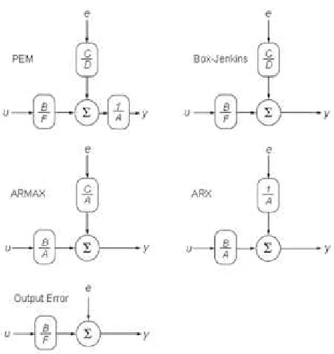
The general structure of black-box model family is proposed in [14] as:

A(q)y(t) = B(q)

F(q)u(t) +

C(q)

D(q)e(t) (2.3)

Specially, various classes of models can be derived from Equation 2.3. As shown in Figure 2.3,

the linear black-models are categorised as Prediction Error Method (PEM) model as shown in

Equation 2.3, the Box-Jenkins (BJ) model whenA= 1, the ARX model whenF =C=D=

(28)

The predictor of the model output can be defined as the regression form in [25]:

ˆ

y(t_|θ) =θTφ(t, θ) (2.4)

[image:28.595.205.443.211.463.2]

where the parameter vectorθ= [θ1, θ2, θ3, ...].

Figure 2.3: Linear black-box model classes

Nonlinear black-box models

The nonlinear black-box model estimator is able to be described as a nonlinear functiong(_·)

of regressor vectorφ(t) and corresponding parameter vectorθ as

ˆ

y(t_|θ) =g(φ(t), θ) (2.5)

In the case of discrete system, the time shift operator q is transformed into z and

the output dynamics of the system is revealed by difference dynamics or tapped delays [6].

Figure 2.4 demonstrates the dynamical model with tapped delays. The past inputs and

outputs of the system can be restored by these delay taps and recycled into the dynamical

(29)

1), y(t₋2)...y(t₋n) are used in the feedback, the dynamical model is named as NARX

(Nonlinear AutoRegressive with eXogenous input) model. On the other hand, if the model

outputs ˆy(t),yˆ(t₋1), ...,ˆ(y₋n) are adopted as the feedback, the model should be categorised

as the NOE (Nonlinear Output Error) Model. From the prospect of model identification, it is

likely that NOE mode will offer better simulation results than that from an ARX or NARX

model which are identified using the measured data.

Figure 2.4: The identified dynamical model with a series of unit tapped delays

Here we define input and output regressor asu(t₋nu),y(t−ny), the model predicted

output as ˆy(t₋ny|θ). Then the simulated output ˆyu(t−ny|θ) can be defined as the model

output ˆyu(t|θ) at time t with all measured outputs y(t−ny) replaced by the simulated

output ˆyu(t−ny)|θ) computed k-step ahead. Therefore, the model prediction error becomes

e(t₋ne) =y(t−ny)−yˆ(t−ny|θ) and the simulation error iseu(t−ne) =y(t−k)−yˆu(t−ny|θ).

Based on these expressions, the corresponding nonlinear version of the model types are

defined as [26, 27]:

• NFIR models which only includes input regressors u(t₋nu)

• NARX models which contain both input and output regressorsu(t₋nu) andy(t−ny)

(30)

• NOE models which useu(t₋nu) and ˆy(t−ny|θ) as regressors when the simulated model output is calculated iteratively as ˆyu(t)|θ)

• NBJ models which adoptu(t₋nu),y(t−ny),e(t−ne|θ) andeu(t−ne|θ) as regressors. In this model class, the simulated output ˆyu is determined by using the structure of

Equation 2.5 at the same time substituting e and eu by zero vectors in the regression

vector φ(t, θ).

2.1.5 Grey-box Models

A comparison between Black-box and White-box models is shown in Fig. 2.2. The white-box

model’s high interpretability is most advantageous, but it requires exact knowledge of the

system. On the other hand, the black-box model is capable of fast simulation of the system but

not interpretable in physical sense. In reality, model identification lies in somewhere between

the two ends. These model classes can be called the Grey-box models which offers higher

flexibility in system identification process. When we has some a priori physical knowledge

about the system but are not able to solve the parameters associated with it, the data-based

black-box approach can be applied. In terms of interpretability, the physical implication of

the model parameters can be retained and assessed by the designer of the control system.

A series of grey-box models, namely neuro-fuzzy systems and semi-physical models can be

found in [28, 29].

2.1.6 Dynamic Engine Calibration

Engine calibration aims to develop the optimal engine operating scheme under varies

restrain-s, such as: emission legislation, fuel consumption and requests from the driver [30]. The best

trade-off are required to be found because these requirements contradict in the engine

mech-anism. Some of the extensive applications of engine dynamical calibration are documented

in [16]. The engine systems is conventionally calibrated by static mapping techniques which

are based on multi-dimensional tables describing the relationship among the engine inputs

and outputs. With more advanced technology being applied to the engine system, the

(31)

Consequently, the calibration time of the engine will be rising enormously due to the curse of

dimensionality. A lot of researchers suggest that the dynamic models are capable to overcome

the shortcomings of the static calibration, mainly the time-consuming experiment [31, 32].

The model-based calibration is introduced to meet the challenge of more advanced

en-gine calibration. The enen-gine properties is represented by mathematical models instead of

look-up tables. The engine control scheme is then developed based on the engine mapping

generated by engine model testing. Consequently, it is essential for the engine model to be

accurate enough to predict the engine dynamic behaviour. Various types of engine models

were investigated extensively by researchers. The examples of physical models of the air, fuel

and mechanical systems can be found in [33, 34]. The neural networks have also been applied

to engine modelling. The manifold pressure and mass flow processes were modelled in [35]

with eternal recurrent networks.

In this thesis, the engine system is recognized as a complex dynamical system which

memorizes its previous states. From this point of view, the calibration of the engine can

be based on a series of dynamic I/O models. With proper designed test cycle, namely New

European Driving Cycle or random walk signal, the engine static or dynamical model can be

developed solely from the information contained in the data set. It can be concluded that

the model-based engine calibration can significantly reduce the pre-production time thus it

(32)

Chapter 3

Experimental and Virtual Test Bed

Setup

This chapter describes the experimental equipment and setup used for investigation of the

identification techniques for multi-model development and local model structure

identifica-tion.

3.1 Ford Port-Fuel-Injected (PFI) Zetec Engine

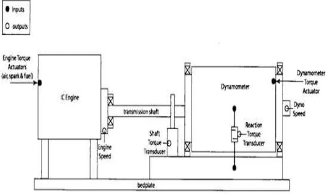
The Liverpool University low inertial dynamometer system installed with Ford Zetec 1.6L PFI

4 cylinder S.I. engine is used for the experimental studies in this thesis. A schematic picture

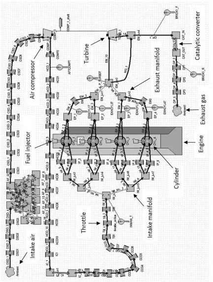
of an engine dynamometer is represented in Figure 3.1. The engine dynamometer system

comprises a test engine and a dynamometer with a connecting transmission shaft. The engine

torque can be controlled by a combination of air, fuelling, spark angle inputs. An in-line

torque transducer is available to measure the torque, and a total reaction torque measurement

arrangement is also available. The other dynamometer parameter is the rotational speed of

the engine shaft and it is measurable by a shaft encoder. A detailed comparison between

PFI and GDI engine mechanism can be found in [36]. The direct injection techniques are

offen used to achieve better fuel dispersion and homogeneity. The control strategies of GDI

combustion is briefly introduced in [37, 38].

(33)

[image:33.595.151.486.115.315.2]

Figure 3.1: A schematic structure of the engine connecting with dynamometer

The results obtained from the engine dynamometer identification provide the data to

determine the effectiveness for any engine modelling or control strategies. Four basic control

modes may be adopted to control the dynamometer [39]:

• Independent Mode: In this mode, the dynamometer torque position is controlled open-loop, which means the disturbances to the model state will not affect the input to the

dynamometer actuator.

• Speed: Here, the speed of the dynamometer is adjusted using closed-loop control with dynamometer speed as the tracked variable.

• Torque: the closed loop system is adopted in this mode to track a desired shaft torque. This mode is useful for the simulation of external loads to increment or decrement the

tracked torque and is obtained by the addition of disturbance signals to the

dynamome-ter torque actuation channel.

• Power: The engine power is determined by the product of torque and rotational speed. Hence the engine power is controlled by adjusting both of them simultaneously.

For identification purposes, the engine system is regarded as a black box. Hence the

main objective of the experiment is to provide the information to reveal the characteristics

(34)

CHAPTER 3. EXPERIMENTAL AND VIRTUAL TEST BED SETUP 20

to collect and record the raw data from the engine test. The data thus obtained from the

experiment are inputs to the identification process to determine the mathematical model

and provide the evidence for the validation of the resulting model. The directly measured

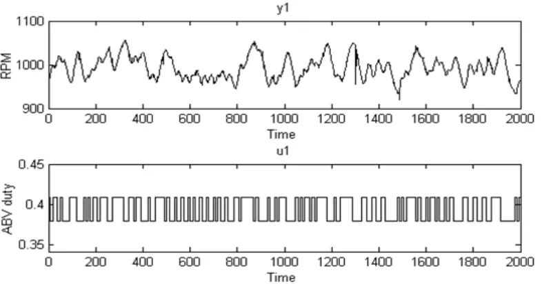
variables include ABV (Air Bleed Valve) Duty Cycle, MAP (Manifold Air Pressure), ABV,

SA and RPM of the engine crank. Among these parameters, for modelling in this thesis, the

ABV Duty Cycle and MAP are regarded as measured input signal while the RPM and UEGO

[image:34.595.168.470.261.481.2]

readingλare chosen as the measured output. The experimental set is shown in Figure 3.2.

Figure 3.2: The key control devices for the engine test

The test engine is a four cylinder engine with four strokes cycle providing four strokes

every 720◦_{. The number of raw data, the samples can achieve 1 million, since samples are}

collected by the software each degree of crank angle. In order to simplify the input control,

the throttle switch is turned off which corresponds to a fixed throttle angle of 8◦_{, thus almost}

all the entered air is bypassed through the ABV. In order to reduce the error, it is necessary

to collect adequate amount of data samples for data processing. Before the test is started, the

engine speed is adjusted to around the idle speed of 1000 rpm and a braking load is applied

by the dynamometer. The dSPACE system is used to collect all the signals and sample them

(35)

3.2 Variable Cam Timing(VCT) Engine

For conventional gasoline engines, the intake and exhaust valves are driven by the camshafts

and the cam timing is adjusted by a timing belt which binds the crankshaft and the camshaft.

By adjusting the phase difference between the camshaft and the crankshaft angle, the timing

belt can synchronize the valve and piston movements in a fixed timing. With optimized

timing of inlet and outlet valve opening in variable valve timing (VVT) engine, the volumetric

efficiency is boosted and the torque output can be increased in all the engine operating regions

thus the fuel economy is improved [40]. Meanwhile, the retard of exhaust valve opening will

reduce or replace the use of exhaust gas recirculation system which would generate more CO

and NOx emissions [41].

Variable Camshaft Timing (VCT) is an automotive variable valve timing technology in

current advanced engines used by many manufacturers including the Ford Motor Coperation.

The VCT technology is an innovation used to minimize the engine emissions whilst providing

also satisfactory fuel economy and driver experience. It has been proved effective and applied

extensively in the industry. This technology has offered considerable merits: it is able to

reduce emissions such as oxides of nitrogen(N Ox) and unburned hydrocarbons(HC) [42],

and also to improve the full load performance of the engine [43]. The specific feature of the

VCT engine, the cam timing is precisely advanced on retarded according to the engine speed

as determined by an optimized engine mapping.

VCT offers another effective way to reduce NOx and HC emissions other than the

ex-haust gas recirculation(EGR) valve systems. However, the VCT mechanism requires more

sophisticated control schemes to achieve the emission reduction target. As shown in Fig 3.3

, the exhaust gas is sucked back in to the cylinder after TDC is reached. The gas mixture

in the cylinder is diluted by the retained exhaust gas which reduces the combustion

temper-ature. Therefore, the NOx generation is suppressed under lower tempertemper-ature. Meanwhile,

the recirculated exhaust gas containing unburned HC from the cylinder or piston wall

inter-face will undergo combustion in the next engine cycle. The camshaft of the VCT engine is

actuated by a hydraulic mechanism and the valve timing is adjusted according to the engine

inlet and exhaust cycle. There are several cam timing schemes, namely Dual Variable Cam

(36)

tim-CHAPTER 3. EXPERIMENTAL AND VIRTUAL TEST BED SETUP 22

ing of Dual-VCT is adjusted simultaneously with the fixed phase differences. On the other

hand, the Ti-VCT adjusts the intake and exhaust camshaft separately in order to produce

higher power and torque and at the same time keep the emissions to a minimum. However,

the Ti-VCT scheme will increase the complexity of the timing actuator and the cost of the

engine.

Figure 3.3: Variable Camshaft Timing scheme

In this thesis, a VCT engine model developed by Stefanopoulou [44] is investigated by

establishing a Matlab Simulink model and simulating the dynamical properties obtained from

the empirical polynomial model given in Stefanopoulou’s work.

The calibration and control target of our study is to maintain the stoichiometric Air/Fuel

Ratio while minimizing the HC and NOx emissions. The key features of the engine, such

as the throttle angle, engine pumping rate, torque generation and NOx and HC emissions

are included as the calibration variables. In detail, the manifold air pressure is physically

determined by the mass flow rate into the throttle body and cylinder as shown in

Equation-s (3.1) (3.2).

Km =

R_·T Vm

= 287

J

Kg·K ·288K

0.007m3 = 0.118bar/g (3.1)

(37)

(288K),Vm represents the manifold volume (0.007m3), andKm is the resulting constant.

The rate of change of the manifold pressure is determined by:

d

dtPm=Km( ˙mθ−m˙cyl) (3.2)

where ˙mθ represents the mass air flow rate into the manifold and ˙mcyl is the engine pumping

mass air flow rate. These two air flow rates can be calculated by Equations (3.3) and (3.4)

respectively:

˙

mθ =g1(Pm)·g2(θ) (3.3)

˙

mcyl=F(1, CAM, CAM2, CAM3, Pm, Pm2, Pm3, N, N2, N3) (3.4)

where CAM is the camshaft angle, N is the engine speed, Pm is the manifold pressure, θ

represents the throttle angle and

g1(Pm) =

  

1 if Pm ≤P0/2, P0= 1 atm

2/P0

p

PmP0−Pm2 if Pm> P0/2

  

(3.5)

and

g2(θ) =F(1, θ, θ2, θ3) (3.6)

The cylinder mass air flow, torque and NOx and HC emissions are modeled by the

static algebraic functions of cylinder air charge (CAC), camshaft angle (CAM), manifold

air pressure (Pm), air/fuel ratio (A/F) and engine speed (N). The schematic output model

structure is outlined in Equation (3.4) (3.7) (3.8) and (3.9):

(38)

N Ox =F1(1, N, N2)·F2(1, CAM)·F3(1, A/F, A/F2, A/F3)·F4(1, Pm, Pm2) (3.8)

HC=F1(1, N, N2)·F2(1, A/F, A/F2, A/F3)·(F3(1,

1

Pm

) +F4(1, CAM,

CAM

P

1 16 m

)) (3.9)

A new Simulink realization which simulates this VCT engine model is shown in

Fig-ure 3.5. The Simulink model is constructed in four subsystems which determine the four-stoke

phases: throttle and manifold intake, air/fuel compression, ignition and combustion, exhaust

generation. Each subsystem has its own physical and empirical sub-models with

correspond-ing inputs and outputs. For the intake system, air flow rate, throttle angle and manifold air

pressure are recognized as inputs. In the final stage, the brake torque is a modelled output

of the combustion system while the NOx and HC emissions are estimated outputs of the

exhaust system.

Figure 3.4: Inputs and Outputs of the VCT Engine

3.3 Diesel Engine with VGT and EGR

Diesel Engines are widely used in heavy-duty vehicles due to its higher torque output and

(39)

Figure 3.5: VCT Engine Simulation Model in Simulink

(40)

Figure 3.7: VCT Engine Torque Model

the turbocharger and the supercharger. However, these two mechanism adopts different

working strategy. The turbochargers utilize the kinetic energy of the exhaust gas flow and

improved the energy efficiency of the engine, but it only works effectively when the engine

operates at relatively high speed. Meanwhile, the superchargers are directly connected with

the crankshaft which is driven by the engine main combustion power, therefore its response

time is shorter and working consistently during the engine operating time. Nevertheless, the

supercharger requires to keep drawing power from the engine which reduce the power and

torque output on the wheels [45].

For the purpose of minimizing the emission within the legislated limit, exhaust

recir-culation and variable-geometry turbochargers have been introduced into the Diesel engine

design. A well-established Diesel engine model which is presented in [46] was adopted as

a test template for the multi-model. This model was peer-reviewed and validated from the

industrially obtained experimental data [47] [48] [49]. As shown in Figure 3.8, eight state

variables are involved in the engine model structure: the intake manifold pressurepim, the

exhaust manifold pressure pem, the intake oxygen mass fraction XOim, the exhaust oxygen

mass fractionXOem, the turbocharger speedωt, and three actuator state variableuδ,uegr,uvgt

where uδ is the mass of injected fuel, uegr represents the EGR valve position and the uvgt

is the VGT valve position. The valve position value varies from 0(closed) to 1(fully open).

(41)

form of Equation 3.11:

u= (uδ uegr uvgt)T (3.10)

whereuδis the injected fuel,uegris the position of EGR valve, anduvgtis the actuator position

of the VGT.

The state-space model:

˙

x=F(x,u, N) (3.11)

where the function F(_·) is developed by combining the dynamic physical properties of all

the key components shown in Figure 3.8 [50]. The dynamic testing of the Diesel engine

was conducted by generating randomly input sequences foruand then observing the output statesxat different engine speed(N) through the time of the test.

Figure 3.8: Inputs and Outputs of the Diesel Engine with VGT mechanism

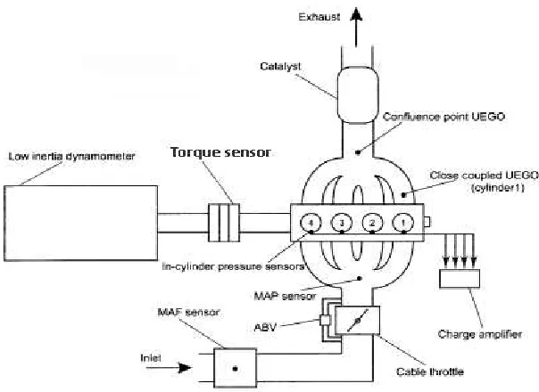
3.4 WAVE-RT Petrol Engine Model

The model structure identification techniques is applied to a high accurate industrially

(42)

disturbances, namely, temperature and moisture, could cause system uncertainty and

com-promise the validation results however in terms of experimental effectiveness, the

computer-aided engine simulator is able to conduct highly repeatable engine test within relative low

time and cost budget. At the same time, the engine model maintains good flexibility to

changing component units and parameters. The subject engine for WAVRT model is an

E-coBoost 2.0-Litre GTDI engine provided by the Ford Motor Co.. The WAVE real-time model

is built on an ISO approved software package named RICARDO WAVE platform [51, 52].

The WAVE platform contains a library of modelling components in the area of

compressible-flow fluid networks and machinery. In terms of engine modelling, it offers elements such

as piston compressor, engine cylinder, throttle, turbocharger and turbine. The time-variant

variables for the engine, including temperature, cylinder pressure and air mass flow rates, can

be measured directly in SI or Imperial units and monitored within the simulation process.

WAVE is recognized as a state-of-the-art industrial design tool and has extensive

appli-cation in engine performance assessment. From early concept studies to detailed engine

pro-duction investigations, the WAVE model can be used throughout the engine design process.

Common applications include torque response, fuel consumption, turbocharger response,

E-GR studies, valve profile design and timing optimization. As shown in Figure 3.9, for the

sake of simplicity of use, the Wave-RT model is mainly comprised of a series of connection

of physical models of engine components along with the engine breathing pipeline, including

throttle and cylinder intake mechanism. As a concept engine design tool, the wave model is

recognized by Ford engineers as a realistic alternative to the real engine for conducting initial

stages of a control scheme. The engine simulation results obtained from the WAVE model

can be plotted in various standard graphical formats and validated by different types of real

(43)

[image:43.595.105.538.138.710.2]

(44)

Chapter 4

Engine SISO Model Identification

4.1 Method of Least Squares Parameter Identification

The methods used for the data processing are the most significant factors which affect the

accuracy and reliability of the identification results. The basic algorithm for parameter

identification, the least-squares algorithm, is introduced in this chapter.

Least-squares (LS) theory was first proposed by Karl Gauss for predicting the orbit of the

planets. Since then, the LS theory has become a principle tool for parameter estimation from

experimental data. The LS method is easy to comprehend and does not require an extensive

knowledge of mathematical statistics; thus it is widely used among scientists and engineers.

Furthermore, estimates obtained by LS methods have optimal statistical properties which are

consistent, unbiased and efficient [11] . Before applying LS theory, the choice of input and

output signal of the system are required to be decided.

4.1.1 Definition of the vector norm

The concept of vector norms is described in the mathematical representation. A vector norm

onRn _{is a function}_f _:_Rn_→_R _{that satisfies the following properties [53]:}

f(x)_≥0 x_∈Rn, (f(x) = 0 if f x= 0) (4.1)

(45)

f(x+y)_≤f(x) +f(y) x, y_∈Rn (4.2)

f(αx) =_|α_|f(x) α_∈R, x_∈Rn (4.3)

Such a function is denoted with a double bar notation: f(x)=_kx_k. With different sub-scripts on the double bar, various norms can be distinguished. Then the p-norms are defined

by:

kx_k_p= (_|x1|p+· · ·+|xn|p) 1

p _p_≥₁ _(4.4)

Three of these norms are the most significant:

kx_k₁ =_|x1|+|x2|+· · ·+|xn| (4.5)

kx_k₂= (_|x1|2+|x2|2+· · ·+|xn|2) 1

2 = (xTx) 1

2 (4.6)

kx_k_∞=max1≤i≤n|xi| (4.7)

Note that a unit vector is a vector x which satisfies_kx_k_p=1.

4.1.2 Least-squares via the minimum error-squares

an n-tuple setX= (x1,x2,· · · ,xn) are related linearly to a variable y:

(46)

CHAPTER 4. ENGINE SISO MODEL IDENTIFICATION 32

whereθ= (θ1, θ2,· · · , θn)T is an n-tuple constants so thaty=Xθ. Let the sum of squares of errors be determined as follows [54]:

J = N

X

t=1

e2(t) =eTe

= (y₋Xθ)T(y₋Xθ)

=yTy₋θTXTy₋yTXθ+θTXTXθ (4.9)

The equation to determine the stationary point for derivation of the minimum of J with

respect toθis:

dJ

dθ =−2X

T_y_{+ 2}_XT_X_θ_{= 0} _(4.10)

which leads to

XTy=XTXθ (4.11)

The second derivative ofJ can be represented as:

d2_J

dθ2 = 2X

T_X _(4.12)

which requires XTX > 0 for a minimum and therefore the stationary point obtained from Equation 4.11 is able to make the sum of squares J minimum. Hence the least square estimator

(LSE) for the polynomial model 4.8 is

xLS = ˆθ=

XTX−1

XTy (4.13)

4.1.3 Least-squares via QR algorithm

Let X _∈ Rm×n _with _m

≥ n and b _∈ Rm and suppose Q _∈ Rm×m _{is an orthogonal matrix}

such that

QT =Q−1

(47)

whereI is the identity matrix. The QR algorithm starts from the matrix formation that

QTX =R=

 

R1,n×1

0(m−n)×1



 (4.15)

where the matrix X is formed asX= [x1, x2, x3..., xn]T and if

QTb=

 

hn×1

g₍m−n)×1



 (4.16)

In the least-squares algorithm, the aim is to determine ˆθwhich is able to minimize_kXθ₋b_k2₂.

Obviously, this problem is equivalent to the minimization ofQTXθ−QTb

2

2. In this case

kXθ₋b_k2₂ =QTXθ−QTb

2

2 =kR1θ−hk 2

2+kgk22 (4.17)

For any x _∈Rn_{, if rank(X)=rank(}_R

1)=n, then ˆθ is defined by the upper triangular system

such that

R1ˆθ=h

ˆ

θ=R−1

1 h (4.18)

Based on this QR Algorithm, the coefficient vector of ˆθ can be obtained.

4.1.4 Least-squares via SVD algorithm

In linear algebra, the SVD is a vital factorization of a rectangular real or complex matrix,

with several applications in signal processing and statistics. Applications which employ the

SVD include computing the pseudo-inverse, matrix approximation, and determining the rank,

(48)

Q and Z are orthogonal matrices such that

QTXZ =T =

 

T11 0r×(n−r)

0₍m−r)×r 0(m−r)×(n−r)



 r =rank(X)

kXθ₋b_k2₂=

(QTXZ)ZTθ−QTb

2

2=kT11a−ck 2

2+kdk22 (4.19)

where in the Equation 4.19,X= [x1, x2, x3..., xn]T,

ZTθ=

 

ar×1

b₍n−r)×1



 QTb=  

cr×1

d₍m−r)×1

 

If the 2-norm ofx is minimum, b must be zero and a=T₁₁−1c. Therefore,

xLS = ˆθ=Z

 

T−1 11 c

0



 (4.20)

4.1.5 Least squares via Recursive Least-Squares (RLS) algorithm

The requirement for recursive solutions arise when fresh experimental data are continuous

in supply and on-line results are required. With recursive formula, the LS estimates can be

updated at each experimental data sample. The recursive methods are often called sequential

or on-line estimation methods.

If the first m groups of data are embedded in matrixXm and ym, then

y_m =Xmθ (4.21)

Hence the least squares estimator can be written as:

ˆ

θ(m) = (XT_mXm)−1XTmym (4.22)

Assume a vector of new experimental datax(m+ 1) and y(m+ 1) are then obtained, where

(49)

if we define

xT(m+ 1) = [x1(m+ 1), x2(m+ 1),· · · , xn(m+ 1)] (4.24)

Then the output of next time point is

y(m+ 1) =xT(m+ 1)θ (4.25)

Consequently, the new data system including the (m+ 1)th equation can be written as

ym+1 =xm+1θ (4.26)

in which

y_m₊₁=

           y(1) y(2) .. .

y(m)

y(m+ 1)

           =            y_m

y(m+ 1)

           (4.27)

Xm+1=

       

x1(1) · · · xn(1) ..

. . .. ...

x1(m) · · · xn(m)

x1(m+ 1) · · · xn(m+ 1)

        =         Xm

xT(m+ 1)

        (4.28)

Hence the new least-squares estimator of next iteration is

ˆ

θ(m+ 1) = [XT_m₊₁Xm+1]−1XTm+1ym+1 (4.29)

Without matrix inversion, the new estimator ˆθ(m+ 1) can be calculated by simply updating

(50)

this. Let A,C and A+BCD be nonsingular square matrices; then the following

Sherman-Morrison-Woodbury formula holds [11]:

(A+BCD)−1 =A−1₋A−1B(C−1+DA−1B)−1DA−1 (4.30)

whereA is n-by-n matrix,U is n-by-k, C is k-by-k and V is k-by-n matrix. If we define the

matrixP(m) as

P(m) = (XT_mXm)−1 (4.31)

then

P(m+ 1) = (XT_m₊₁Xm+1)−1 = (XTmXm+x(m+ 1)xT(m+ 1))−1 (4.32)

Applying the matrix inversion lemma described in Equation 4.30, let A = P(m)−1_, _B ₌

x(m+ 1), C= 1 and D=xT₍_m_{+ 1), then} _P₍_m_{+ 1) can be written as follows:}

P(m+ 1) = [P(m)−1+x(m+ 1)xT(m+ 1)]−1=P(m)₋

P(m)x(m+ 1)[1 +xT(m+ 1)P(m)x(m+ 1)]−1xT(m+ 1)P(m) (4.33)

From Equation 4.27 and 4.28

XT_m₊₁y_m₊₁=XT_my_m+x(m+ 1)y(m+ 1) (4.34)

Substituting Equation 4.32 and 4.34 into Equation 4.29, the following relation holds:

ˆ

θ(m+ 1) =P(m+ 1)[XT_my_m+x(m+ 1)y(m+ 1)] = (P(m)₋P(m)x(m+ 1)[1 +xT(m+ 1)P(m)x(m+ 1)]−1

(51)

The above equation can be transformed into

P(m)XT_my(m)₋P(m)x(m+ 1)[1 +xT(m+ 1)P(m)x(m+ 1)−1

·xT(m+ 1)P(m)XT_my_m+P(m)x(m+ 1)y(m+ 1)

−P(m)x(m+ 1)[1 +xT(m+ 1)P(m)x(m+ 1)]−1

·xT(m+ 1)P(m)x(m+ 1)y(m+ 1) (4.36)

The last two terms of Equation 4.36 can then be rearranged into the form

P(m)x(m+ 1)[1 +xT(m+ 1)P(m)x(m+ 1)]−1

·[1 +xT(m+ 1)P(m)x(m+ 1)

−xT(m+ 1)P(m)x(m+ 1)]_·y(m+ 1)

=P(m)x(m+ 1)[1 +xT(m+ 1)P(m)x(m+ 1)]−1_y₍_m_{+ 1)} _(4.37)

From Equation 4.22 and 4.31, the following relations can be obtained:

ˆ

θ(m) =P(m)XT_my_m (4.38)

Finally, the ˆθ(m+ 1) can be written as

ˆ

θ(m+ 1) = ˆθ(m)₋P(m)x(m+ 1)[1 +xT(m+ 1)P(m)x(m+ 1)]−1

·xT(m+ 1)P(m)XT_mym +P(m)x(m+ 1)[1 +xT(m+ 1)P(m)x(m+ 1)]−1y(m+ 1) = ˆθ(m) +P(m)x(m+ 1)[1 +xT(m+ 1)P(m)x(m+ 1)]−1

·[y(m+ 1)₋xT(m+ 1)ˆθ(m)] (4.39)

The result obtained in Equation 4.39 shows that the next estimator is calculated by the

previous one plus a correction term. Therefore, the recursive least-squares estimation can be

executed by the following equations:

ˆ

Model structure selection in powertrain calibration and control

Calibration and Control

Thesis submitted in accordance with the requirements of the

University

of

Liverpool

for the

Degree of Doctor in Philosophy

by

Zongyan Li

Statement of Originality

Abstract

Contents

List of Figures

List of Tables

Introduction

1.1

Systems identification of SISO and MIMO models

1.2

Overview

1.3

Contributions

Chapter 2

Background

2.1

Dynamical System Identification for IC Engine

Chapter 3

Experimental and Virtual Test Bed

Setup

3.1

Ford Port-Fuel-Injected (PFI) Zetec Engine

3.2

Variable Cam Timing(VCT) Engine

3.3

Diesel Engine with VGT and EGR

3.4

WAVE-RT Petrol Engine Model

Chapter 4

Engine SISO Model Identification

4.1

Method of Least Squares Parameter Identification