Boolean-controlled systems via receding horizon and linear programing.

White Rose Research Online URL for this paper:

http://eprints.whiterose.ac.uk/89742/

Version: Accepted Version

Article:

Bauso, D. (2009) Boolean-controlled systems via receding horizon and linear programing.

Mathematics of Control, Signals, and Systems (MCSS), 21 (1). 69 - 91. ISSN 0932-4194

https://doi.org/10.1007/s00498-009-0038-3

[email protected] https://eprints.whiterose.ac.uk/ Reuse

Unless indicated otherwise, fulltext items are protected by copyright with all rights reserved. The copyright exception in section 29 of the Copyright, Designs and Patents Act 1988 allows the making of a single copy solely for the purpose of non-commercial research or private study within the limits of fair dealing. The publisher or other rights-holder may allow further reproduction and re-use of this version - refer to the White Rose Research Online record for this item. Where records identify the publisher as the copyright holder, users can verify any specific terms of use on the publisher’s website.

Takedown

If you consider content in White Rose Research Online to be in breach of UK law, please notify us by

Dario Bauso

Boolean-controlled systems via

receding horizon and linear

programming

Received: date / Revised: date

Abstract We consider dynamic systems controlled by boolean signals or de-cisions. We show that in a number of cases, the receding horizon formulation of the control problem can be solved via linear programming by relaxing the binary constraints on the control. The idea behind our approach is concep-tually easy: a feasible control can be forced by imposing that the boolean signal is set to one at least one time over the horizon. We translate this idea into constraints on the controls and analyze the polyhedron of all feasible controls. We specialize the approach to the stabilizability of switched and impulsively-controlled systems.

Keywords Impulse Control·Inventory Control·Hybrid Systems

1 Introduction

Hybrid optimal control problems are, in general, difficult to solve (see, e.g., [10; 13; 29] and references therein). For this reason, a current research goal is toisolate those problems that lead to tractable solutions [10]. According to this aim, in this paper we identify among the larger set of hybrid optimal control problems dealt in [13], a special class of problems which are easy to solve. Easy to solve means that the solution algorithms are polynomial in time and therefore suitable to the on-line implementation in real-time

This work was supported by MURST-PRIN 2007ZMZK5T “Decisional model for the design and the management of logistics networks characterized by high inter-operability and information integration”.

D. Bauso

Dipartimento di Ingegneria Informatica Universit`a di Palermo, Viale Delle Scienze, 90128 Palermo, Italy.

problems. We do this by using a paradigm borrowed from the Operations Research field.

More precisely, this paper is one of the several recent attempts [1; 2; 4; 5; 13] to apply the tools of combinatorial optimization to hybrid optimal control problems. The general recipe is to take the standard continuous-time hybrid optimal control problem, discretize it, and reformulate and massage it until it is suitable for applying one of the several discrete optimization techniques [4; 5]. Integer programming, or one of its variations, seems to be specially favorite for this line of research.

In Section 2, we consider systems characterized by a continuous state, a binary state, and controlled through a binary control. The binary state describes the two operating modes of the system while the binary controls represent resets, impulses, or switches between modes. The problem consists in finding feasible controls, i.e., controls that satisfy certain stabilizability conditions.

Boolean control/decision spaces can be found in finite-alphabet control and in particular on-off control problems [16], impulsively-controlled systems (activate the impulse or not) [10; 20], or switching control (switches be-tween active and passive modes) [21; 22; 26]. Applications include inventory with set up costs (reordering or not from a warehouse in order to meet a demand) [8], distributed computer systems (processing or not the assigned task) [15], air-conditioning systems control, economics and finance (see, e.g., [9] and references therein).

The main result of this work is stated in Section 3. There, we show that in many cases the receding horizon formulation of the problem can be solved via linear programming after relaxing the binary constraints on the control and exploiting the total unimodularity of the constraint matrix [11; 14; 24]. This is the case anytime a feasible solution derives from imposing that the control is set to one at least one time in the horizon window.

In Section 4, we specialize the approach to the (asymptotic) stabilizability of switched systems. Two cases are considered: time dependent slow switching controls and state dependent switching controls. As illustrative example, we simulate a switched oscillating system under different feasible solutions.

In Section 5, we extend the approach to the Input to State Stabilizability (ISS) of impulsively controlled systems, according to the definition provided in [20]. In particular, we focus on ISS systems with dwell time and reverse dwell time. As illustrative example, we simulate a first order system under different feasible solutions.

In Section 6, we extend the discussion to inventory applications and in Section 7, we draw some conclusions.

2 Problem formulation

2.1 Boolean-controlled systems

q=0 q=1 u=1

u=1

u=0 u=0

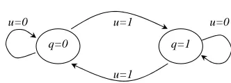
Fig. 1 Transitions between mode 1 and 2.

Equation (1) describes a switched system where q ∈ {0,1} is a binary state (the operating modes), functionfq :Rn×Rm 7→Rn is the dynamics in mode q of x(t), the binary control u(t)∈ {0,1} for all t ≥0 describes a switching control returning a switch wheneveru(t) is set to one. Transitions of the binary state from one mode to the other one are described by the automata displayed in Fig. 1:

˙

x(t) =fq(x(t), d(t)),

q(t+_{) =}

½

q(t) ifu(t) = 0 1−q(t) ifu(t) = 1.

(1)

Equation (2) describes an impulsively-controlled system where function

f : Rn_×Rm_{7→ R}n _{is the dynamics of x(t), h(x(t), d(t)) is the reset value,}

u(t) is the impulse control law returning impulses wheneveru(t) is set to one:

˙

x(t) =f(x(t), d(t)) ifu(t) = 0

x(t+_{) =h(x(t), d(t)) ifu(t) = 1.} (2)

Let an additional function V :Rn _{7→R be given. For instance, one may} think V(x(t)) being a differentiable norm function. We wish to solve the following problem.

Problem 1 Find a controlu(t)∈ {0,1}for allt≥0 such that the following condition is satisfied

ψ(V(0), V(t),V˙(t))>0, (3)

whereψ:R×R×R7→Ris a generic function ofV(0),V(t), and ˙V(t).

We use ˙V(t) to indicate the derivative ofV at timet.

In Section 4, condition (3) reduces to ˙V(t) <0 (negative derivative) as we focus on asymptotic stabilizability of a switched system (see also the switching-based Lyapunov function approach in [12]). Similarly in Section 5 condition (3) describes the Input to State Stabilizability (ISS) condition for an impulsively-controlled system (see the ISS conditions introduced in [20]).

2.2 Receding horizon

Let a finite set of times {r0, . . . , rh} be arbitrarily chosen and consider a receding horizon from timerito timeri+1, withi= 0, . . . , h−1 (control and prediction horizons coincide). Take a sample interval∆t= ri−ri−1

timesri+k∆twithk= 0, . . . , N. Let the discrete time continuous and binary states be ξ(k), andζ(k) respectively with the initial conditionξ(0) =x(ri) andζ(0) =q(ri). Also, let the discrete time controlµ(k) and disturbanceγ(k) be obtained by samplingu(t) andd(t) at timeri+k∆t, i.e.,µ(k) =u(ri+k∆t) andγ(k) =d(ri+k∆t).

Then, fork= 0, . . . , N−1, the sampled counterpart of system (1) is

ξ(k+ 1) =ξ(k) +wζ(k)(ξ(k), d(t)), ξ(0) =x(ri)

ζ(k+ 1) =

½

ζ(k) ifµ(k) = 0

1−ζ(k) ifµ(k) = 1 ζ(0) =q(ri)

µ(k) ∈ {0,1},

(4)

where wζ(k)(ξ(k), d(t)) = Rri

+(k+1)∆t

ri+k∆t fζ(k)(x(t), d(t))dt. Here we indicate

d(t) as explicit argument of wζ(k)(·) to mean thatwζ(k)(·) depends on the whole functiond(t) over the interval fromri+k∆ttori+ (k+ 1)∆t. Anal-ogously to the continuous time case, the condition µ(k) = 1 means that a switch occurs at timeri+k∆twhereasµ(k) = 0 means that the binary state is unchanged.

Analogously, the sampled counterpart of system (2) is

ξ(k+ 1) =ξ(k) +w(ξ(k), d(t))+

+ (h(ξ(k), γ(k))−ξ(k))µ(k), ξ(0) =x(ri)

µ(k) ∈ {0,1},

(5)

where we denote by

w(ξ(k), d(t)) =

Z ri+(k+1)∆t

ri+k∆t

f(x(t), d(t))dt. (6)

Again,d(t) as explicit argument ofwζ(k)(·) means that wζ(k)(·) depends on the whole function d(t) over the interval from ri +k∆t to ri + (k + 1)∆t. We can relax conditions (3) by considering the following discrete time counterpart, fork= 0, . . . , N−1

ψ(V(ξ(0)), V(ξ(k+ 1)), V(ξ(k+ 1))−V(ξ(k)))>0. (7)

Feasible solutions for fixed horizon [ri, ri+1], areu,d,x, andqthat satisfy (4) or (5), (6) and (7) where we define

u= [µ(0), . . . , µ(N−1)]d= [γ(0), . . . , γ(N−1)] x= [ξ(0), . . . , ξ(N)] q= [ζ(0), . . . , ζ(N)].

For a compact description, define the feasible solution set

F(q(ri), x(ri)) ={u,d,x,q∈ {0,1}N ×RN×m× ×R(N+1)×n× {0,1}N+1_{: (4) or (5), and (7) satisfied}.}

Now, given the setH={0, . . . , N}of possible values of the indexk span-ning over the horizon window, consider a generic set of subsets{C1, . . . , Cm} such thatS_jCj =H and eachCj is made by consecutive elements ofH, i.e., given any pair y, z ∈Cj with y < z this impliesv ∈Cj for anyy < v < z and for allj= 1, . . . , m.

We claim that in a number of cases (some of these cases are discussed in Section 4 and 5) there exists a specific set of subsets {C1, . . . , Cm} with

m ≤ N such that condition (7) is satisfied if at the initial time ri of the horizon and under certain conditions on the initial statesq(ri), x(ri) of the horizon, we impose that the following constraints on the binary controls hold

true _X

k∈Cj

µ(k)≥lj(q(ri), x(ri)), for allj= 1, . . . , m (8)

where function lj : {0,1} ×Rn → {0,1} models some logical conditions for

q(ri) and x(ri). In all these situations we can get rid of d, x, and q and rewrite the feasible solution set in a simplified manner as shown below

F(q(ri), x(ri)) ={u∈ {0,1}N : (8) satisfied}.

Rewriting the solution set as above has the advantage of converting the original dynamic problem (because of the presence of the state variable) into a static one. This is possible as in a receding horizon setting, variablesq(ri) and x(ri) once measured at time ri enter as parameters in the right-hand side of (8).

To complete the formulation of the receding horizon problem, let the following vector of costs of the switching controls over the horizon be given

c= [c0, . . . , cN−1]T.

The receding horizon problem is then

min

u∈F(q(ri),x(ri))

cTu. (9)

Finally, once obtained the optimal sequence of discrete controlsµ(0), . . . , µ(N− 1), we need to reconstruct the continuous time controlsu(t). We can do this through the following functionθ:{0,1}N _{7→ {u(t), r}

i≤t < ri+1}returning, for each interval [ri+k∆t, ri+ (k+ 1)∆t), the control u(ri+k∆t) =µ(k) andu(t) = 0 for allt∈(ri+k∆t, ri+ (k+ 1)∆t).

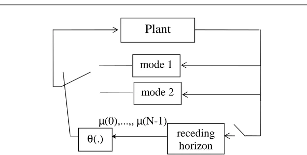
Figure 2 displays the closed-loop system with a switched static feedback. At timerithe receding horizon controller selects and implements the controls

µ(0), . . . , µ(N−1) based on the current state x(ri), q(ri). The procedure is repeated at timeri+1 on the bases of the new state updatex(ri+1), q(ri+1).

3 Main result

Plant

mode 1

receding

horizon

θ

(.)

µ

(0),...,,

µ

(N-1)

mode 2

Fig. 2 Closed-loop system with switched static feedback: at timeri the receding

horizon controller selects and implements the controlsµ(0), . . . , µ(N−1) based on the measured statex(ri), q(ri). The procedure is repeated at timeri+1on the bases

of the new state updatex(ri+1), q(ri+1).

points. However we can replace the integrality constraints u ∈ {0,1}N _by the relaxed and more tractable constraints 0 ≤ u ≤ 1 and consider the resulting polytope

P(q(ri), x(ri)) ={u∈RN :

X

k∈Cj

µ(k)≥lj(q(ri), x(ri)),∀j= 1, . . . , m,0≤u≤1}.

We clarify this aspect more in details next. Let us rewrite the inequali-ties (8) in matrix form. We can do this by using a matrix A ∈ {0,1}m×N_, with only entries 0 and 1, one row for each inequality of type (8), one column for each timek. Observe that the constraint matrix is aninterval matrix, i.e., it has 0-1 entries and each row is of the form

(0, . . . ,0 1, . . . ,1

| {z } 0, . . . ,0).

consecutive 1’s

It is well known from the literature [24] that each interval matrix is totally unimodular where we remind here that a matrix istotally unimodular if the determinant of any square sub-matrix is equal to−1, 0 or 1. We report next a simple proof.

Lemma 1 Any interval matrix Ais totally unimodular.

Proof We need to show that any generic square sub-matrix R ∈ {0,1}p×p ofA is such thatdet(R)∈ {0,±1}. Take the incidence matrix of a directed chain graph withpnodes (its determinant is equal to one)

Z:=

     

1−1 0 . . .0 0 0 1 −1. . .0 0 ..

. ... ... . .. ... ... 0 0 0 . . .1−1 0 0 0 . . .0 1

and compute the matrixL:=ZRT_{. One can see thatLis still an incidence} matrix of a directed graph as each column ofLhas either only one non null element (1 or−1) or just a 1 and−1 and the rest are zero elements. To see this, take thejth column of L,

L•j = (Z1•R_•jT, . . . , Zp•RT•j)T

and observe that thejth column of RT _{has the following structure}

RT

•j = (0, . . . ,0, 1

|{z}

¯ith element

, . . . , 1

|{z}

¯

jth element

,0, . . . ,0)T_.

Then, we derive that L(¯i−1)j = Z(¯i−1)•R•jT = −1, L¯jj = Z¯j•RT•j = 1 and

Lij = Zi•RT•j = 0 for all i 6= ¯i−1,¯j. With a little abuse of notation the same argument can be used to prove that the column L1• has only one non null element equal to −1 (here note that ¯i = 1). This proves thatL is still an incidence matrix of a directed graph also that det(L) ∈ {0,±1} or which is the same that Lis totally unimodular. Then we can conclude that

det(R) =det(Z)det(RT_{) =det(L)∈ {0,±1}. ⊓⊔}

This means that the polytope P obtained fromF by replacing the inte-grality constraints µ(k)∈ {0,1} with the linear constraint 0 ≤µ(k)≤1 is an integral polyhedron. As a consequence we have that the linear relaxation of the receding horizon problem (9) has an integral optimal solution as es-tablished in the next theorem. Let the vector of logical conditions be defined asl= [l1(q(ri), x(ri)), . . . , lm(q(ri), x(ri))]T.

Theorem 1 Solving the receding horizon problem (9) is equivalent to solving the linear programming problem

min

u

cT_{u (10)}

s.t. Au≥l (11)

0≤u≤1. (12)

Proof Apply a standard technique in linear programming to turn the con-straints (11) into equalities of type

[A I]

·

u s

¸

=l (13)

where s ∈ Rm _{is the surplus vector and I ∈R}m×m _{is the identity matrix.} From the properties of total unimodular matrices one knows that ifAis to-tally unimodular then also [A I] is totally unimodular. Then, take a generic square sub-matrixR ∈Rm×m _{and observe that det(R) ∈ {0,±1}. Any} ad-missible base solution of (13) is of the form ¯v=R−1_l=adj(R)

4 Switched systems

In this section, we show that the paradigmatic problem (10)-(12) suits to the (asymptotic) stabilizability of switched systems. To do this, we can take for

V(x(t)) any differentiable norm function and simplify equation (3) as ˙V <0. Two cases are considered next: time dependent slow switching controls and state dependent switching controls. For the switched system (1) we wish to solve the following problem.

Problem 2 Find a switching controlu(t)∈ {0,1}for allt≥0 such that the origin is asymptotically stable.

4.1 Time dependent slow switching controls

Let us focus on systems that are stabilizable through a time dependent slow switching control. In particular, assume that there exists a (minimum)dwell time T. Minimum dwell time means that for guaranteeing ˙V <0 it suffices that the time interval between two successive switches is at leastT. Details on how to computeT for specific classes of problems can be found in [21; 22]. Consider the sampled counterpart (4) starting at time ri, take for sim-plicity ∆t= 1, and assume that ri−ˆk is the time of the last switch. The following linear programming problem of type (10)-(12) returns a switching control satisfying the above dwell time condition:

minucTu, s.t. 0≤u≤1,

 

b

z }| {

1. . . .1 0. . .0 0. . . .0 1. . .1

 

| {z }

A

  

µ(0) .. .

µ(N−1)

  

| {z }

u

≥

·

0 1

¸

|{z}

l

, (14)

whereb=T−kˆ. The above problem derives from takingC1={1, . . . , T−kˆ}, andC2={(T−ˆk)+1, . . . , N}. Note that the above constraint matrixAdoes not exclude multiple switchings between (T −ˆk) + 1 andN which possibly violate the dwell time condition. However such solutions though admissible, are not optimal for problem (10)-(12) as multiple switchings increase the cost.

The receding horizon process repeats at time ri+1 =ri+N ∆t (regular starting times) or at timeri+1=ri+ (˜k+ 1)∆twhere ˜kis the last switching time returned by the problem solved at timeri(time-varying starting times).

4.2 State dependent switchings

In particular, let us consider two open conic regions Π1 and Π2 which overlap and such thatΠ1SΠ2=Rn\ {0}.

Assume that there exists a hysteresis-based stabilizing switching of the type described in [22] and recalled next. For each t > 0, ifq(t−_{) = 0 and}

x(t)∈Π1, keepq(t) = 0. Differently, ifq(t−) = 0 butx(t)6∈Π1, then assign

q(t) = 1. Analogously, ifq(t−_{) = 1 andx(t)∈Π}

2, keepq(t) = 1. Differently, ifq(t−_{) = 1 butx(t)6∈Π}

2, then assignq(t) = 0.

Now, we can approximate the above hysteresis-based switching control by using the linear programming problem (14). To see this, consider the sampled counterpart (4) starting at timeri, and letri+b∆tas the expected time to cross a pre-defined surfaceS ∈Π1TΠ2.

The optimal solution of (14) returns no switches between 0 and b, and only one switch betweenb+ 1 andN−1, i.e.,

µ(0) =. . .=µ(b) = 0, µ(b+ 1) +. . .+µ(N−1) = 1. (15)

The length of the interval [b+ 1, N] describes how long it takes for a switch to occur once the state has crossed the surfaceS. In the special case where

N = b+ 1, the surface S turns out to be a switching surface as a switch occurs any time the surfaceS is crossed.

4.2.1 Oscillating systems

Consider the second order systems

·

˙

x1 ˙

x2

¸

=

·

0 1 −κ(q) 0

¸ ·

x1

x2

¸

where q ∈ {0,1} is the mode and with spring coefficient κ(0) = 1 (pas-sive control) andκ(1) = 2 (aggressive control). The binary state transition function is as in (1).

It is well known that switching law of type (16) asymptotically stabilizes the system at the origin [22]:

q(t) =

½

0 ifx1(t)x2(t)≤0

1 ifx1(t)x2(t)>0 . (16)

This corresponds to having two switching surfaces S1 ={x∈R2: x1 = 0} andS2={x∈R2: x2= 0}(see, e.g., Fig. 3).

We can approximate a switching law of type (16) as shown next. First consider the sampled counterpart of the above system. To do this denote by

ω(q) =pκ(q). Sampling is possible after defining the following two compo-nents vector,

wζ(k)(ξ(k)) =

     

ξ1(k) cos(ω(ζ(k))∆t)+ +( ξ2(k)

ω(ζ(k))) sin(ω(ζ(k))∆t)−ξ1(k)

−ξ1(k)ωsin(ω(ζ(k))∆t) + (_ωξ₍2_ζ(₍k_k)₎₎)· ·ω(ζ(k)) cos(ω(ζ(k))∆t)−ξ2(k)

     

with initial conditionξi(0) =xi(ri),i= 1,2, and where the two components predict the evolution of position and velocity respectively.

Now, letri+b∆tbe the expected time to cross the surfaceS1ifq(ri) = 0. Similarly, letri+b∆tbe the expected time to cross the surfaceS2ifq(ri) = 1. To approximate the switching law of type (16) it suffices to takeN =b+ 1 whereb has the meaning discussed above. Actually, the linear programming problem (14) returns a switch any time one of the surfaces S1 and S2 is crossed.

A slight modification in the choice of N may return the asymptotically stabilizing hysteresis-based switching control discussed next (see, Fig. 3). Take for a small enoughα >0

Π1={x∈R2: x1x2<0}S{x∈R2: x2> αx1},

Π2={x∈R2: x1x2>0}. (17)

The overlapping region is Π1TΠ2 = {x∈ R2 : x1x2 > 0, x2 > αx1} (grey region), the surface S3 = {x2 = αx1} describes the boundary of Π1 while the surface S2 describes the boundary of Π2. Now take ri such that

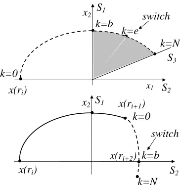
x(ri)∈Π1 and q(ri) = 0. Compute ri+b∆t as the expected time to cross the surfaceS1or takeb= 0 if the state has already crossedS1(that is,x(ri) is already inΠ1TΠ2). Also takeN as the expected time to cross the surface S3. Then the linear programming problem (14) returns only one switch when the state is in the overlapping region Π1TΠ2. Let the time of the switch be ri+e∆t. Note that the resulting switching control is again of type (15). Fig. 3 top, displays the predicted state trajectory (dashed line) from point

ξ(0) = x(ri) on the x1-axes (also surface S2) to point ξ(N) on surface S3. In evidence point ξ(b) = x(ri+b∆t) on the x2-axes (also surfaceS1), and pointξ(e) =x(ri+e∆t) when the switch occurs. At the next iteration of the receding horizon procedure, we take ri+1 :=ri+ (e+ 1)∆t. Now, we have

x(ri+1) ∈ Π2 and q(ri+1) = 1. Compute ri+1+b∆t as the expected time to cross the surface S2 and take N =b+ 1. Then, the linear programming problem (14) returns only one switch immediately after the state has crossed S2. Fig. 3 bottom, displays the current state trajectory fromx(ri) tox(ri+1) (solid line) and predicted state trajectory (dashed line) from point ξ(0) =

x(ri+1) to point ξ(N). In evidence pointξ(b) =x(ri+b∆t) on the x1-axes (also surfaceS2) when the switch occurs. We can repeat the procedure when the state is in the second and third quadrant. The resulting hysteresis-based switching control is such that there exists a periodically decreasing quadratic functionV(x) (if we keep the passive control mode, i.e.,q(t) = 0 for allt, the trajectory describes an ellipsoid with main axes parallel to the x1x2-axes). Actually, from Fig. 3 it is evident thatV(x(ri+2))−V(x(ri))<−βx(ri) for a small enough β >0. The above condition is a sufficient condition for the asymptotical stability of the system at the origin.

k=N

S

x(r

)

S

k=e

switch

x

S

x(r

)

S

switch

x

x(r

)

S

k=N

x(r

)

k=0

k=0

k=b

k=b

Fig. 3 Two successive iterations of the receding horizon procedure: (top) predicted trajectory (dashed line) at theith iteration; (bottom) current trajectory (solid line) and predicted trajectory (dashed line) at thei+ 1st iteration. FunctionV(x(t)) is periodically decreasing.

−1 0 1

−1 −0.5 0 0.5 1 x 1 x2

−1 0 1

−1 −0.5 0 0.5 1 x 1 x 2

−1 0 1

−1 −0.5 0 0.5 1 x 1 x2

−1 0 1

−1 −0.5 0 0.5 1 x 1 x2

−1 0 1

−1 −0.5 0 0.5 1 x 1 x 2

−1 0 1

−1 −0.5 0 0.5 1 x 1 x2

Fig. 4 Trajectories in thex1x2-plane under different feasible solutions.

5 Impulsively-controlled systems

In this section, we show that the paradigmatic problem (10)-(12) suits to the Input to State Stabilizability (ISS) of impulsively controlled systems, according to the definition provided in [20].

To do this, we can take for V(x(t)) any differentiable norm function and consider equation (3) as a reformulation of condition (2) in [20].

In particular, we focus next on ISS systems with dwell time and reverse dwell time. For the impulsively-controlled system (2) we wish to solve the following problem.

Problem 3 Find an impulse control law u(t) (i.e., a sequence of impulse times t1,t2. . . , tk, . . .) such that system (2) is input to state stable (ISS) according to the definition of [20].

5.1 (Reverse) dwell time

In [20] it has been shown that for a number of systems Problem 3 can be solved by any impulse control law u(t) satisfying some so-called (reverse) dwell time conditions. A typical dwell time condition requires that intervals between consecutive impulses must be no shorter than T time units. All these cases can be dealt with exactly as shown in Section 4.1. On the con-trary, a typical reverse dwell time condition requires that intervals between consecutive impulses must be no longer thanT time units. We can generalize the approach by consideringmdifferent dwell timesT1, T2, . . . , Tmover the horizon as shown next.

Consider the sampled counterpart (5) starting at time ri, take for sim-plicity∆t= 1, and assume that ri−1 is the time of the last impulse. The following linear programming problem of type (10)-(12) returns a switching control satisfying the above reverse dwell time condition:

minucTu, s.t. 0≤u≤1,

       T1

z }| {

1. . .1 0. . .0 . . .

Tm

z }| {

0. . .0 0 1. . . .1 . . .0. . .0

..

. . .. ... 0. . .0 0. . .0 . . .1. . .1

      

| {z }

A    µ(0) .. .

µ(N−1)

  

| {z }

u ≥    1 .. . 1   

| {z }

l

. (18)

The above problem derives from taking C1={0, . . . , T1}, C2={1, . . . ,2 +

T2}, . . ., Ci = {i−1, . . . , i+Ti}, . . ., Cm = {m−1, . . . , N}. In the next section, we apply the approach to a first-order system.

5.1.1 First order system Consider system

˙

x=a(t)x(t) +rand(−1,1)

| {z }

f(x(t),d(t))

with ratea(t)>0 and whererand(−1,1) is a random disturbance uniformly distributed in the interval between−1 and 1, andsat(.) is the typical linear saturated (at−1 or 1) function. The sat(.) function derives from taking

h(., .) =

½

x(t)−sign(x(t)) if|x(t)|>1 0 if|x(t)| ≤1 .

We simulate a one step (fromri= 0 tori+1) receding horizon procedure. The number of setsCi ism= 27.

We take as initial state x(ri) = x(0) = 9. Let us take as time unit the value −log((ǫ−1)/ǫ) = 0.0953 where ǫ = 11 is an upper bound of |x(t)|. This value derives from the fact that between two consecutive impulses we can guarantee the condition |x(ri+1)| ≤ ǫ−_ǫ1|x(ri)| at least on the average because of the random disturbancerand(−1,1) (the same condition is always guaranteed in absence of a random disturbance). The sample interval is ₁₀1 of the time unit−log((ǫ−1)/ǫ), i.e., ∆t=−log((ǫ−1)/ǫ)0.1 = 0.00953.

Now, the rate is a(t) = 0.1 for 0 ≤ t < 14 (during intervals Ci, with

i = 1, . . . ,15) and a(t) = 0.2 for 14 ≤ t < 20 (during intervals Ci, with

i= 16, . . . ,27). The reverse dwell time is computed following the procedure in [20] as Tj = # of steps for time unit_{rate in C}

j and the result is Tj =

10

0.1 = 100, for j = 1, . . . ,15 and Tj = ₀10_.2 = 50 for j = 16, . . . ,27. It follows that the horizon length isN = 14·100 + 12·50 = 2100.

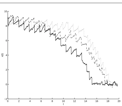
Figure 5 shows the time plot ofx(t) when impulses occur at the beginning of each interval (solid line). This happens when costs are increasing, that is,

c1 < c2 ≤. . . ≤cN−1, or also when costs are increasing over each interval

Ci={Pi−

1

j=1Tj+1, . . . ,Pi−

1

j=1Tj+Ti}, i.e.,cr< . . . < cswithr=Pi−

1

j=1Tj+1 and s = Pi−_j=11Tj +Ti. The figure also shows the time plot of x(t) when impulses occur in the middle of each interval (dotted line). This happens when on each intervalCi={Pi−j=11Tj+ 1, . . . ,Pji−=11Tj+Ti}we havecr< cs for allr6=swith r=Pi−_j=11Tj+T₂i. Finally, the figure shows the time plot ofx(t) when impulses occur at the end of each interval (dash-dot line). This happens, for instance, when costs are decreasing, that is, c1 ≥ c2 ≥ . . . >

cN−1 or also when costs are decreasing over each interval Ci={Pi−_j=11Tj+ 1, . . . ,Pi−_j=11Tj +Ti}, i.e., cr ≥ . . . > cs with r = Pi−j=11Tj + 1 and s =

Pi−1

j=1Tj+Ti. In all of the three cases the system is ISS stable as the state

x(t) is driven in a neighborhood of the origin whose sizes depend on the maximal amplitude of the random disturbance.

6 Inventory examples

0 2 4 6 8 10 12 14 16 18 20 −2

0 2 4 6 8 10

t

x(t)

Fig. 5 Time plot ofx(t) when impulses occur at the beginning of each intervalCi,

i= 1, . . . ,27 (solid line), in the middle of each interval (dotted line), and at the end of each interval (dash-dot line).

for the exchange rate [17; 18] (see, e.g., [6] for an exhaustive list of appli-cations). The first example can be found also in [6] and [10], Example 3.5, and in [2]. The second example provides a more generic interpretation of the impulsively-controlled system (2), which is now used to describe a controlled switched multi–inventory system (see, e.g., [1]).

6.1 Inventory ([6] and [10], Example 3.5)

With in mind the impulsively-controlled system (2), let the state x(t) ∈R

describe the inventory level, let functionV(t) =x(t) and use (3) to impose the conditionx(t)≥s, wheresis the lower inventory threshold. Resetsu(t) describe the choice of the retailer of reordering, in which case the inventory is restored at level S = h(x(t), d(t)), or not reordering. Costs of resets c

are transportation costs. Let f(x(t), d(t)) = −d(t) where d(t) ∈ D ⊆ R is the (nonnegative) demand faced by the retailer. Then, equation (9) is the minimization of transportation costs, equation (2) is the evolution of the in-ventory and equation (3) prevents the inin-ventory to be lower than thresholds. The sample interval is the minimum time occurring between two consecutive reorders.

6.2 Switched multi–inventory systems

Consider the family of continuous time linear multi–inventory systems

˙

x(t) =Biuc(t)−d(t), i∈ {1, . . . ,Q} (19)

wherex(t)∈IRn is a vector whose components are the buffer levels,uc(t)∈ IRmis the controlled flow vector,Bi∈Qn×mis the controlled process matrix andd(t)∈IRn is the unknown demand. To model backlogx(t) may be less than zero. Controls and demands are bounded within polytopes according to

uc(t)∈ Uc={uc∈Rm:u−c ≤uc ≤u+c} (20)

d(t)∈ D={d∈Rn:d−≤d≤d+}, (21)

whereu−

c ,u+c,d−, andd+ are assigned vectors. We also assume that matrix

Bi is a “fat matrix” and has full row rank.

For the above switched multi–inventory system, the notion of unstable mode can be reviewed as follows. We say that each system ˙x(t) =Biuc(t)−

d(t) (henceforth simply system Bi), is an unstable mode if there no exists feedback stabilizing strategies [3], that is, strategies able to drive the state within a neighborhood of a reference value x_{ref of radius} ǫ in finite time. This is true if the polytope of demand is not contained in the image of the polytope of controls via Bi, i.e., D 6⊆ int{BiU}. Henceforth, assume that only BQ satisfies the above condition, namely, D ⊆ int{BQU} and that D 6⊆int{BiU}, i= 1, . . . ,Q −1. In the following, we refer to systems

B1, . . . , BQ−1 as the unstable modes whereas we refer to systemBQ as the stable mode.

After introducing the stable and unstable modes, the switched multi– inventory system is alternatively in one of theQmodes as described by the following dynamics

˙

x=PQ_i=1αi(t)(Biuc(t)−d(t))

PQ

i=1αi(t) = 1, binary.

(22)

Transitions between successive unstable modes are autonomous and in accor-dance to a given sequence (only unstable modes are in the sequence) whereas transitions from an unstable mode to the stable mode are controlled by the switching signalµ(k)∈ {0,1}fork= 0, . . . , N−1. More precisely, let us call

kthepoch the time interval betweent(k) andt(k+ 1) where

t(k+ 1) =t(k) +Tµ(k) +∆t, (23)

the two logical operators “and” and “not”, transitions are governed by the following expressions. For allk= 0, . . . , N −1

[t=t(k)]∧[µ(k) = 1]∧[ασ(k−1)(t) = 1]→[αQ(t+) = 1] (24) [t=t(k)]∧[µ(k) = 0]∧[ασ(k−1)(t) = 1]→[ασ(k)(t+) = 1] (25) [t=t(k) +T]∧[αQ(t) = 1]→[ασ(k)(t+) = 1]. (26)

Conditions (24) and (25) describe transitions at the beginning of the kth epoch from modeBσ(k−1)toBQifµ(k) = 1 and toBσ(k)(successive mode in the sequence) ifµ(k) = 0, respectively. Condition (26) describes the transition from mode BQ to Bσ(k) after a time interval of T (throughout this paper we always assume that, for the stable mode, a time interval of lengthT is large enough to drive the statexwithin a neighborhood of zero). Finally, the following condition says that in all the other circumstances no transitions occur:

∼¡[t=t(k)]∧[ασ(k)(t) = 1] ¢

∧ ∼([t=t(k) +T]∧[αQ(t) = 1])→[αi(t+) =αi(t)].

(27)

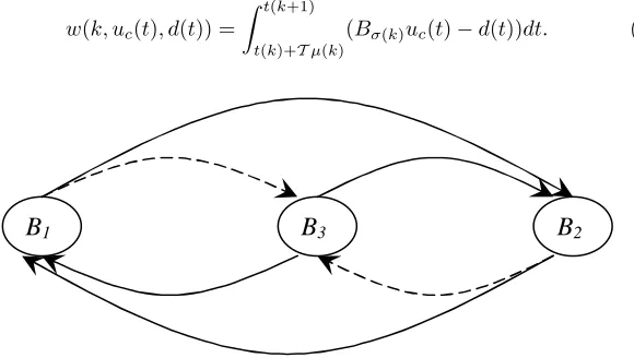
Figure 6 displays controlled and uncontrolled transitions (arcs) among modes (nodes) for Q= 3. Figure 7 displays the time plot for a one dimen-sional state. In evidence the epoch (sampling interval) betweent(3) andt(4) which has a size of∆t+T.

To put the above model in the form (5), we need to slightly modify the definition of the state dependent disturbance in (6) and the sampling rule introduced in Section 2.2. Actually, now, the disturbance is no longer state dependent, and sampling occurs at the beginning of each epoch, where the epochs are defined as in (23). Given this, we only need to change the notation

w(ξ(k), d(t)) intow(k, uc(t), d(t)) and also to specify that if at time t(k) a switch occursµ(k) = 1 then one extreme of the integral (6) is shifted forward ofT, i.e.,

w(k, uc(t), d(t)) =

Z t(k+1)

t(k)+Tµ(k)

(Bσ(k)uc(t)−d(t))dt. (28)

B

B

B

Fig. 6 Transitions among different modes: nodes represent unstable modesB1and B2 and stable modeB3. Arcs describe controlled transitions (dashed) to the stable

Henceforth, we simply writew(k, uc, d) instead of w(k, uc(t), d(t)).

Then, the problem of interest consists in finding the optimal schedule of the switches among unstable and stable modes thus to maintain the system in a safe operating region, while minimizing a function related to the cost of the switches. In this case, the cost of a switch represents the cost of driving the state to the origin, once a transition to the stable mode has occurred (in the assumption that such a cost is independent of the value of the state at the time of the transition). The decision variables are thus binary (whether to switch to the stable mode at a given time instant or not).

With in mind the sampling rule (23) and the new definition ofw(k, uc, d) as in (28) the sampled multi–inventory model reduces to

ξ(k+ 1) =ξ(k) +w(k, uc, d) + (x_ref−ξ(k))µ(k) µ(0) = 1, (29)

the above equation being a specialization of (5).

Now, assume that we wish to keep the state within a neighborhood of a reference valuex_{ref of size}ǫ. Assumex(0) is already in the neighborhood and takex_{ref = 0 without loss of generality. We can formalize the above concept}

by considering, for instance, V(x) =kxk∞. LetX ={x∈Rn : V(x)≤γ} for a given thresholdγ∈R+ withRn+ the positive orthant. Condition (7) is then simply

V(ξ(k+ 1))≤γ, k= 0, . . . , N−1. (30)

With this in mind, the generic setCj used in (8) can be defined as follows.

x

t(1)

ε

switch

γ

∆t

T

∆t

_t(2)

_t(3)

∆t

_t(4)

t

Definition 1 Set Cj ={¯k,¯k+ 1, . . . ,˜k−1,˜k} is made up by consecutive time instants such that, forx(¯k) =x_{ref, it holds}

min uc(.)∈Uc

max d(.)∈D V

 

˜

k

X

k=¯k

w(k, uc, d)



> γ (31)

min uc(.)∈Uc

max d(.)∈D V

 

˜

k−1

X

k=¯k

w(k, uc, d)



≤γ. (32)

SetsCj’s define the minimal time intervals which must be “covered” by at least one reset, for a solution uto be feasible under the worst disturbance. Difficulties in computing the setsCj’s are discussed in the next section.

6.2.1 Computation of sets Cj’s

With in mind the fact that the disturbance is, for this system, state inde-pendent (see, e.g., (28)) and in the assumption that, for the computation of setsCj’s, no switch occurs between times ¯kand ˜k, we must solve a min-max optimization problem of type

z∗_{= min} uc(.)∈Uc

max d(.)∈DV

 

˜

k

X

k=¯k

w(k, uc, d)



. (33)

Note that (33) is the same as the first term of (31). Also, we can imme-diately observe that the costV ³P˜k_k=¯kw(k, uc, d)

´

is convex. Now, in state of solving (33) consider the following greedy min-max problem (the indexg

reminds “greedy”). Find the solution of

zg= ˜

k

X

k=¯k

µ

min uc(.)∈Uc

max

d(.)∈DV (w(k, uc, d))

¶

. (34)

Note that the greedy problem (34) is obtained from (33) by simply in-verting the “min max” with the “sum”. Denote by (u∗

c(t), d∗(t)), the solution of (33), i.e.,

u∗c(t) = arg min uc(.)∈Uc

V   ˜ k X

k=¯k

w(k, uc, φ(uc))



 (35)

d∗(t) =φ(u∗c(t)), (36)

where the functionφ(uc) = arg maxd(.)∈D V

³P˜_k

k=¯kw(k, uc, d)

´

. Analogously, denote by (ug

c(t), dg(t)), the solution of each term of the sum in (34), that is

ug

c(t) = arg min uc(.)∈Uc

V(w(k, uc, φ(uc))) (37)

where for each intervalt(k)≤t≤t(k+ 1), the function

φg_(u

c) = arg max

d(.)∈D V (w(k, uc, d)). (39) Associate to (u∗

c(t), d∗(t)) and (ugc(t), dg(t)) the corresponding distur-bance and state

w∗_{(k) =}

Z t(k+1)

t(k)

(Bσ(k)u∗c−d

∗_{)dt, ξ}∗_{(k) =}Pk−1

r=¯kw ∗

j(r), (40)

wg(ξ(k)) =

Z t(k+1)

t(k)

(Bσ(k)ugc−dg)dt, ξg(k) =

Pk−1

r=¯kw

g_{(r). (41)}

In other words, (40)-(41) are the disturbances and states for the two problems (33) and (34) respectively.

Note that, we have denoted the first extreme in the two above integrals simply byt(k) rather thant(k) +Tu(k) as for the computation of setsCj’s, we always assume that no switch occurs between times ¯kand ˜k. Finally, let

t(ˆk) = arg maxt(r),r=1,...,Nt(k)≤t. Then, the continuous time state can be obtained as

ξ∗(t) =ξ∗(ˆk) +

Z t

t(k)

(Bσ(k)u∗c−d ∗

)dτ (42)

ξg_{(t) =ξ}g_{(ˆk) +}

Z t

t(k)

(Bσ(k)ugc −dg)dτ. (43)

We are now ready to establish the exactness of the greedy computation.

Theorem 2 For the multi–inventory system of Section 6.2 it holdszg_=z∗_. Proof First, observe that for the multi–inventory system of Subsection 6.2,

V(.) is convex and w(k, uc, d) is linear on d(t). As a consequence of this, the worst demand d∗ _{and the greedy demandd}g _{are on a vertex ofD. We} specialize the proof to the case where the state trajectory is in the negative orthant. We wish to show thatξg_{(k) =ξ}∗_{(k) for allk= ¯k, . . . ,}˜_{k. First note} that provingξg_(k)≥ξ∗_{(k) for all k= ¯k, . . . ,k˜ derives straightforwardly by} the definition ofd∗ _{and d}g_{. Now, we prove by induction thatξ}g_(k)≤ξ∗_(k) for allk= ¯k, . . . ,˜k. Actually, fork= ¯k, we haveξ(¯k) = 0 andwg_(¯k)≤w∗_(¯k). The two latter conditions implyξg_{(¯k+ 1)≤ξ}∗_{(¯k+ 1). Now, for anyk <˜k,} assumeξg_(k)≤ξ∗_{(k) and prove ξ}g_{(k+ 1)≤ξ}∗_{(k+ 1). To do this, observe} that, ifξg_{(k+ 1)> ξ}∗_{(k+ 1) then there must exist a timet witht(k)< t≤}

t(k+ 1) such thatξg_{(t) =ξ}∗_{(t) and ˙ξ}g_(t)>ξ˙∗_{(t). But this is possible only} if d∗ _{> d}g _{= d}+ _{which contradicts the assumption d}− _{≤ d ≤ d}+_{. We can} conclude thatξg_{(k) =ξ}∗_{(k) for allk= ¯k, . . . ,˜kand alsoz}g_=z∗_{. ⊓⊔}

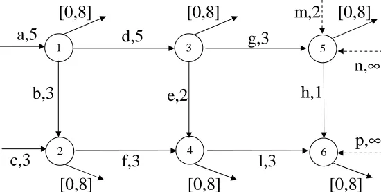
6.2.2 Numerical Example

See the switched multi–inventory system in Fig. 8. Brackets [0,8] indicate the minimum and maximum demand at the nodes. Maximum capacity for each arc is specified below the name, i.e., “a,5” means that arc ahas maximum capacity equal to 5. Minimum capacity is 0 for all arcs. Topology 1 has only arc a, b, . . . , l, topology 2 has the additional arcmand topology 3 has additional arcs m, n and p. The corresponding incidence matrices are as follows (B2 is obtained fromB1 adding the only column of arcm)

B3=

B1

z }| {

      

1−1 0−1 0 0 0 0 0 0 1 1 0 0−1 0 0 0 0 0 0 1−1 0−1 0 0 0 0 0 0 1 1 0 0−1 0 0 0 0 0 0 1−1 0 0 0 0 0 0 0 0 1 1

m,n,p

z }| {

0 0 0 0 0 0 0 0 0 0 0 0 1 1 0 0 0 1

      

Let us also assume that the total demand (summed over all 6 nodes) is at most equal to 8, that is,P_i=1,...,6di≤8. Then, from (38) the greedy demand isdg _{= [0,0,0,0,8,0]}T _{for topology 1 and d}g _{= [0,0,0,0,0,8]}T _{for topology} 2. Also, from (37) the greedy flows areug

c = [3,0,0,3,0,0,3,0,0]T andugc = [1,0,3,1,0,3,1,1,3]T _{for topology 1 and 2 respectively. Assume∆t= 1, from} (41), we obtain wg_{(k) = [0,0,0,0,5,0]}T _{for topology 1 (namely, fork such} that σ(k) = 1), andwg_{(k) = [0,0,0,0,0,4]}T _{for topology 2 (namely, for k} such thatσ(k) = 2).

Observe that only systemB3isǫ-stabilizable (it satisfiesD ⊆int{B3U}), whereas systemsB1 andB2 are not.

Assume that the system switches autonomously between topology 1 and 2 according to a uniformly distributed random sequence.

1

2

3 5

4 6

a,5

b,3

c,3

d,5

e,2

g,3

f,3

h,1

l,3

m,2

n,

∞

p,

∞

[0,8]

[0,8]

[0,8]

[0,8]

[0,8]

[0,8]

Also, assume that at any reset the system switches on B3 so that the buffer length can be driven within a neighborhood of 50. We also force the buffer to be non negative (no backlog). Then set x_{ref = 50 and} γ = 50. Over the horizon of length N = 100, the costs of the resets are increasing (controlled switches toB3occur at the end of each interval) in the first case and decreasing in the second case (controlled switches to B3 occur at the beginning of each interval).

Once the system has switched toB3, the controlled flow in the additional arcsnandpis of typeuc,11(t) =x_ref−x5(t) anduc,12(t) = 0.2(x_ref−x6(t)) respectively. For sake of simplicity we assume that when modeB3 is active, the demand is of typed(t) = [0,0,0,0,8,0]. With the above choice ofuc,11(t) andd(t), the system is stabilizable within a neighborhood of size 8 (equal to the maximal demand at node 5). The initial state isx5(t) =x6(t) =x_{ref =} 50.

IfV(.) is the∞-norm, we can computekwg_(k)k

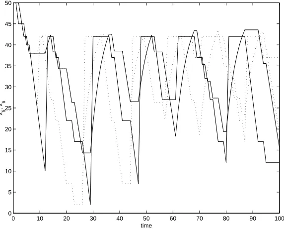
∞for eachk. From (34) we can compute the setsCj’s, and derive a set of 100 inequalities of type (8) that enter as constraints in the linear programming problem (10)-(12) returning the optimal control sequence (controlled switches). Such a sequence is used to simulate the state evolution of Fig. 9 in the two cases of decreasing (solid line) and increasing (dashed line) costs.

7 Conclusions

Hybrid optimal control problems are, in general, difficult to solve. A current research goal is to isolate those problems that lead to tractable solutions. In this paper, we have identified among the larger set of hybrid control problems a special class of optimal control problems which are easy to solve. Easy to solve means that solution algorithms are polynomial in time and therefore suitable to the on-line implementation in real-time problems. We have done this by using a paradigm borrowed from the Operations Research field.

References

1. D. Bauso, “Optimal switches in multi–inventory systems”, in Proc. of the10th International Conference on ”Hybrid Systems: Computation and Control” -HSCC ’07, Pisa, Italy, 2007, pp. 641–644.

2. D. Bauso, R. Pesenti, “A Polynomial Algorithm solving a Special Class of Hybrid Optimal Control Problems”, in Proc. of the IEEE Conference on Control and Applications, Munich, Germany, Oct. 4-6, 2006, pp. 349–354.

3. D. Bauso, F. Blanchini, R. Pesenti, “Robust control strategies for multi-inventory systems with average flow constraints”, Automatica, vol. 42, no. 8, pp. 1255–1266, Aug. 2006.

4. A. Bemporad and M. Morari, “Control of systems integrating logic, dynamics, and constraints”,Automatica, vol. 35, pp. 407-427, 1999.

5. A. Bemporad, S. Di Cairano and J. J`ulvez, “Event-driven optimal control of integral continuous hybrid automata”, in Proc of 44th Control and Decision Conference and European Control Conference 2005, Seville, Spain, pp. 1409– 1414.

7. D. P. Bertsekas, I. Rhodes, “Recursive state estimation for a set-membership description of uncertainty”, IEEE Transactions on Automatic Control vol. 16, no. 2, pp. 117–128, 1971.

8. D. Bertsimas, A. Thiele, “A Robust Optimization Approach to Inventory The-ory”,Operations Research, vol. 54, no. 1, January-February 2006, pp. 150-168. 9. E. Boros and P. L. Hammer, “Pseudo-Boolean optimization”,Discrete Applied

Mathematics, vol. 123, pp. 155-225, 2002.

10. M. S. Branicky, V. S. Borkar and S. K. Mitter, “A Unified Framework for Hybrid Control: Model and Optimal Control Theory”, IEEE Transactions on Automatic Control, vol. 43, no. 1, pp. 31–45, 1998.

11. A. Caprara, M. Fischetti and P. Toth, “Algorithms for the Set Covering Prob-lem”,Annals of Operations Research, vol. 98 pp. 353–371, 2000.

12. D. Casagrande, A. Astolfi and T. Parisini, “Switching-based Lyapunov Func-tion and the StabilizaFunc-tion of a Class of Non-Holonomic Systems”, in Proc. of the

10th International Conference on ”Hybrid Systems: Computation and Control”

- HSCC ’07, Pisa, Italy, 2007.

13. C. G. Cassandras, D. L. Pepyne and Y. Wardi, “Optimal control of a class of hybrid systems”, IEEE Transactions on Automatic Control, vol. 46, no. 3, pp. 398-415, 2001.

14. O. L. V. Costa, “Impulse control of piecewise-deterministic processes via lin-ear programming”, IEEE Transactions on Automatic Control, vol. 36, no. 3, pp. 371–375, Mar 1991.

15. P. R. De Waal and J. H. Van Schuppen, “A class of team problems with discrete action spaces: optimality conditions based on multimodularity”,SIAM Journal

0 10 20 30 40 50 60 70 80 90 100

0 5 10 15 20 25 30 35 40 45 50

time

x5

, x

6

Fig. 9 Time plot of x5(t) and x6(t) in the cases of increasing (solid line) and

decreasing (dotted line) costs. Any time a controlled switch to modeB3occurs, the

on Control and Optimization, vol. 38, pp. 875–892, 2000.

16. G.C. Goodwin and D.E. Quevedo, “Finite alphabet control and estimation”,

International Journal of Control, Automation, and Systems, vol. 1, no. 4, pp. 412–430, 2003.

17. M. Jeanblanc-Piqu´e, “Impulse control method and exchange rate”,Math. Fi-nance, vol. 3, 1993, pp. 161–177.

18. R. Korn, “Optimal Impulse Control when Control Actions have Random Con-sequences”, Mathematics of Operations Research, vol. 22, no. 3, Aug. 1997, pp. 639–667.

19. J. M. Harrison, T. M. Sellke, and A. J. Taylor, “Impulse Control of Brownian Motion”,Mathematics of Operations Research, vol. 8, no. 3, Aug. 1983, pp. 454– 466.

20. J. Hespanha, D. Liberzon, A. Teel, “Lyapunov Characterizations of Input-to-State Stability for Impulsive Systems”, Automatica, vol. 44, no. 11, pp. 2735– 2744, Nov. 2008.

21. D. Liberzon and A. Morse, “Basic Problems in Stability and Design of Switched Systems”,IEEE Control Systems Magazine, vol. 19, no. 5, pp. 59–70, 1999. 22. D. Liberzon,Switching in Systems and Control, Birkhauser, 2003.

23. R. R. Lumley and M. Zervos, “A Model for Investments in the Natural Resource Industry with Switching Costs”, Mathematics of Operations Research, vol. 26, no. 4, Nov. 2001, pp. 637–653.

24. G. L. Nemhauser, and L. A. Wolsey,Integer and Combinatorial Optimization, John Wiley & Sons Ltd, New York, 1988.

25. S. Sridhar, “Determination of aggregate preventive maintenance programs us-ing production schedules”,Computers ind. Engng, vol. 14, no. 2, pp. 193–200, 1988.

26. D. C. Tarraf, A. Megretski and M. A. Dahleh, “A Framework for Robust Sta-bility of Systems Over Finite Alphabets”, IEEE Transactions on Automatic Control, vol. 53, no. 5, pp. 1133– 1146, June 2008.

27. H. M. Wagner, and T. H. Whitin, “Dynamic version of the economic lot-size model”,Management Science, vol. 5, pp. 89–96, 1958.

28. L. A. Wolsey, “Progress with single-item lot-sizing”,European Journal of Op-erational Research, vol. 86, pp. 395–401, 1995.