This is a repository copy of
The formation of very wide binaries during the star cluster
dissolution phase
.
White Rose Research Online URL for this paper:
http://eprints.whiterose.ac.uk/120264/
Version: Accepted Version
Article:
Kouwenhoven, M.B.N., Goodwin, S.P., Parker, R.J. et al. (3 more authors) (2010) The
formation of very wide binaries during the star cluster dissolution phase. Monthly Notices
of the Royal Astronomical Society, 404 (4). pp. 1835-1848. ISSN 0035-8711
https://doi.org/10.1111/j.1365-2966.2010.16399.x
[email protected]
https://eprints.whiterose.ac.uk/
Reuse
Unless indicated otherwise, fulltext items are protected by copyright with all rights reserved. The copyright
exception in section 29 of the Copyright, Designs and Patents Act 1988 allows the making of a single copy
solely for the purpose of non-commercial research or private study within the limits of fair dealing. The
publisher or other rights-holder may allow further reproduction and re-use of this version - refer to the White
Rose Research Online record for this item. Where records identify the publisher as the copyright holder,
users can verify any specific terms of use on the publisher’s website.
Takedown
If you consider content in White Rose Research Online to be in breach of UK law, please notify us by
arXiv:1001.3969v1 [astro-ph.GA] 22 Jan 2010
The formation of very wide binaries during the star cluster
dissolution phase
M. B. N. Kouwenhoven
1,2⋆†
, S. P. Goodwin
2, Richard J. Parker
2, M. B. Davies
3,
D. Malmberg
3and P. Kroupa
41Kavli Institute for Astronomy and Astrophysics at Peking University, Yi He Yuan Lu 5, Hai Dian District, Beijing 100871, P.R. China 2University of Sheffield, Hicks Building, Hounsfield Road, Sheffield S3 7RH, United Kingdom
3Lund Observatory, Box 43, SE-221 00, Lund, Sweden
4Argelander Institute for Astronomy, University of Bonn, Auf dem H ¨ugel 71, 53121 Bonn, Germany
Accepted —. Received —; in original form —
ABSTRACT
Over the past few decades, numerous wide (>103au) binaries in the Galactic field and halo have been discovered. Their existence cannot be explained by the process of star formation or by dynamical interactions in the field, and their origin has long been a mystery. We explain the origin of these wide binaries by formation during the dissolution phase of young star clusters: an initially unbound pair of stars may form a binary when their distance in phase-space is small. Using N-body simulations, we find that the resulting wide binary fraction in the semi-major axis range 103au < a <0.1 pc for individual clusters is 1
−30%, depending on the initial conditions. The existence of numerous wide binaries in the field is consistent with ob-servational evidence that most clusters start out with a large degree of substructure. The wide binary fraction decreases strongly with increasing cluster mass, and the semi-major axis of the newly formed binaries is determined by the initial cluster size. The resulting eccentricity dis-tribution is thermal, and the mass ratio disdis-tribution is consistent with gravitationally-focused random pairing. As a large fraction of the stars form in primordial binaries, we predict that a large number of the observed “wide binaries” are in fact triple or quadruple systems. By integrating over the initial cluster mass distribution, we predict a binary fraction of a few per cent in the semi-major axis range 103au<a<0.1 pc in the Galactic field, which is smaller than the observed wide binary fraction. However, this discrepancy may be solved when we consider a broad range of cluster morphologies.
Key words: Binaries: general – star clusters – methods: N-body simulations
1 INTRODUCTION
A significant fraction of stars in the Galactic field are in bi-nary and multiple systems (e.g, Duquennoy & Mayor 1991; Fischer & Marcy 1992; Mason et al. 1998; Shatsky & Tokovinin 2002; Goodwin & Kroupa 2005; Kobulnicky & Fryer 2007; Kouwenhoven et al. 2005, 2007; Lada 2006; Zinnecker & Yorke 2007; Goodwin et al. 2007). It is also thought that the majority of stars are born in star clusters (Lada & Lada 2003). Therefore the majority of binaries1 in the field population presumably originate
from clustered star formation.
⋆ E-mail: [email protected]; s.goodwin@sheffield.ac.uk; [email protected]; [email protected], [email protected], [email protected]
† Peter and Patricia Gruber Foundation Fellow
1 For brevity we will use ‘binaries’ to mean ‘multiples’ of any
multiplic-ity for the remainder of this paper, only drawing a distinction where it is necessary.
It is well known that binaries are dynamically processed in star clusters with wider and less bound systems tending to be de-stroyed by encounters (Heggie 1975; Hills 1975). Therefore, the field binary population is dynamically processed with respect to the birth population of binaries (Kroupa 1995; Parker et al. 2009). The origin of most field binaries can be understood as a mixture of differently processed initial populations (Goodwin 2009).
However, a significant number of very wide (a>103au)
Many very wide binaries have separations comparable to the average interstellar separation in clusters (typically a few 103au),
and the very widest binaries have separations of order the size of a young cluster core (typically a few 104au). Given this, it is difficult
to see how they could even form, let alone survive, in a cluster (see, e,g., Scally et al. 1999; Parker et al. 2009). Even in an isolated star forming region the typical size of a star forming core is only 104au
(Ward-Thompson et al. 2007) which presumably sets the very max-imum size of a (primordial) binary system.
It is possible that a wide binary forms via dynamical interac-tions in the Galactic field (the capture mechanism). A prerequisite for this mechanism to work is that a significant amount of kinetic energy is dissipated. This energy dissipation can occur due to tidal friction and due to three-body interaction. Tidal friction occurs in the rare event of two stars nearly colliding in a close encounter. In the vast majority of the cases this results in a merger or a fly-by, and only in a small number of cases does this lead to the formation of a binary system. However, all binaries resulting from capture by tidal friction are very tight, with orbital period of several days.
Another possible mechanism is three-body interactions. In this case the third star acts as the energy sink, and is generally ejected with high velocity. However, the stellar density in the field is low, of order 0.1 M⊙pc−3, so that three-body encounters are rare, and
cap-ture by dynamical friction rarely occurs. Goodman & Hut (1993) find that the creation rate ˙NB for binaries per unit volume can be
approximated by
˙
NB=0.75
G5M5n3
σ9 v
, (1)
where M is the typical mass of a star in the field, n the number den-sity of stars,σvthe velocity dispersion, and G the gravitational
con-stant. In the solar neighbourhood M ≈0.3 M⊙, n ≈0.03pc−3and
σv≈50 km s−1. For the field therefore, ˙NB≈4×10⁻²¹pc−3Gyr−1.
This shows that the formation of binaries in the field is extremely rare. Note that in dense star clusters the stellar density is high and the velocity dispersion modest, such that the number of bi-naries formed via three-body interactions (Eq. 1) may be substan-tial. However, wide binaries, which have semi-major axes compa-rable to the size of these clusters, are not formed, as they simply do not fit in these star clusters. Furthermore, N-body simulations by Kroupa & Burkert (2001) have shown that the observed broad period distribution of binaries in the field cannot be produced by dynamically modifying a tighter period distribution in a star clus-ter.
A third possibility for the origin of wide binaries is formation during cluster dissolution, which is the mechanism we propose in this paper. In an evolving star cluster, stars that are initially un-bound, may become bound to each other as the cluster expands, i.e., if the gravitational influence of the other cluster members de-creases2. In order to form a binary pair in this way, (i) the two stars
need to be sufficiently close together, (ii) the two stars need to have a sufficiently small velocity difference, and (iii) the newly formed binary should not be destroyed by gravitational interaction with the remaining cluster stars or field stars.
Throughout this paper we refer to binaries with 103au<a<
0.1 pc as the wide binary population. The paper is organised as
2 Interestingly, Levison et al. (2009) have independently proposed that
large populations of comets may be captured by stars during cluster dis-solution, by a mechanism which is similar to that discussed in this paper for wide binary formation (see also Eggers et al. 1997).
10
210
310
410
5Semi-major axis (au)
1
10
100
Semi-major axis distribution
PAH2007
LB2007
DM1991 CRC1990
CG2004 Halo
[image:3.612.322.542.97.293.2]CG2004 Disk 103 au 0.1 pc 0.2 pc
Figure 1. The observed semi-major axis distribution, f (a), of the wide binary population (in arbitrary units). The curves indicate the Duquennoy & Mayor (1991) distribution (assuming a mass of 1 M⊙for
each binary), and the results from Close et al. (1990), L´epine & Bongiorno (2007) (for both the Galactic disk and halo), Chanam´e & Gould (2004), and Poveda et al. (2007).
100 102 104 106 108 1010
Period P0 (days)
0.0 0.2 0.4 0.6 0.8 1.0
Fraction of binaries with P > P
0
10-2 100 102 104
Semi-major axis a0 (AU)
0.0 0.2 0.4 0.6 0.8 1.0
Fraction of binaries with a > a
0 0.1 pc0.2 pc
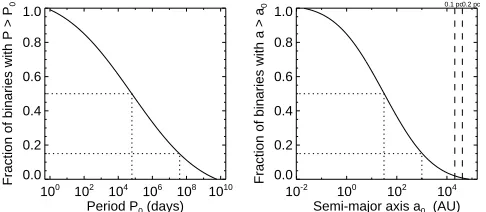
Figure 2. The cumulative distributions in period and semi-major axis for solar-type stars in the solar neighbourhood, for the Duquennoy & Mayor (1991) log-normal period distribution. The total mass of each binary is as-sumed to be MT=1 M⊙. The dotted lines indicate the median semi-major
axis, and a=103au.
follows. In§2 we briefly discuss surveys of wide binary systems and the corresponding observational techniques. In§3 we explain our technique and assumptions. In§4 we provide analytical and Monte Carlo estimates for the resulting wide binary population, and in§5 we present estimates based on N-body simulations of evolving star clusters. Finally, in§6 we present and discuss our conclusions.
2 OBSERVATIONS OF WIDE BINARIES
Observations have indicated that binaries as wide as 1 pc exist in the halo, while in the Galactic disc the widest binaries have separations of order 0.1 pc (e.g., Close et al. 1990; Chanam´e & Gould 2004). Wider binaries are rare, although some authors claim evidence for binary and higher-order multiple systems wider than 0.1 pc (e.g., Scholz et al. 2008; Caballero 2009; Mamajek et al. 2009).
[image:3.612.318.561.395.501.2]of-ten recovered using the angular two-point correlation function (e.g., Bahcall & Soneira 1981; Garnavich 1988; Gould et al. 1995; Longhitano & Binggeli 2010). The most prominent disadvantages of this method are the inability to identity individual wide bina-ries and the need for a good model for the stellar population that is studied.
Individual wide binary candidates are often identified by their common proper motion on the sky (e.g., Wasserman & Weinberg 1991; Chanam´e & Gould 2004; L´epine & Bongiorno 2007; Makarov et al. 2008, and numerous others). Many wide binaries were found by Hipparcos (ESA 1997) as well; see also S¨oderhjelm (2007). Their nature can then be further constrained by mea-suring the parallax and radial velocity (e.g., Latham et al. 1984; Hartigan et al. 1994; Quinn et al. 2009).
The most well-known survey for binarity is arguably that of Duquennoy & Mayor (1991), who carried out a large binarity study for solar-type stars in the solar neighbourhood. They found a log-normal period distribution f (P) with a meanhlog Pi= 4.8 and a standard deviation σlog P = 2.3, where P is the orbital period in
days, in the range 1 . P . 1010days. Note that the latter value
roughly corresponds to an orbital period of 30 Myr. In this log-normal period distribution, ∼ 15% of the binaries have a semi-major axis wider than 103au (see Fig. 2).
Several observational studies suggest a semi-major axis distri-bution of the form f (a) ∝a−1, which corresponds to a flat
distri-bution in log a, also known as ¨Opik’s law ( ¨Opik 1924; van Albada 1968; Vereshchagin et al. 1988; Allen et al. 2000; Poveda & Allen 2004). In particular, Poveda et al. (2007) find binaries in the field follow ¨Opik’s law in the separation range 100.a.3000 au, and suggest that a population of very young binaries follows ¨Opik’s law up to a≈45 000 au (0.2 pc).
Many other authors have also found significant wide bi-nary populations, notably Close et al. (1990), L´epine & Bongiorno (2007), and Chanam´e & Gould (2004). We summarise the wide bi-nary separation distribution from various authors in Fig. 1.
The reliability of the observed properties of wide binary pop-ulations remains an issue. It is difficult to confidently establish whether the two components of a candidate wide binary are truly bound, or whether it is merely a chance superposition. Due to the long orbital periods of wide binaries, up to millions of years, it is impossible to accurately derive orbital properties and therefore confirm the bound state of the candidate wide binary. It should be noted that due to the lack of detailed orbital information, the quoted separations of wide binaries are usually the instantaneous angular separation. The true separations may thus be significantly larger than the observed, projected separations. On the other hand, an es-timate for the semi-major axis distribution of an ensemble of binary systems can statistically be obtained from the projected separation (e.g., Leinert et al. 1993).
On the other hand, it is extremely difficult to identify binaries with distant and faint stellar or substellar companions, due to con-fusion with foreground and background stars (e.g., Chandrasekhar 1944). The wide binary fraction as identified in the observational papers may therefore be a lower limit, rather than an upper limit.
Although the exact form of the semi-major axis distribution for very wide binaries is not yet known (see Fig. 1), two features appear to be clear: (i) the binary fraction in the separation range 103au<a <0.1 pc is roughly 15%, and (ii) a sharp drop-offin
the separation range 0.1−0.2 pc is present, likely due to dynamical destruction of the most weakly bound binary systems.
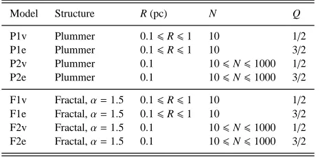
Model Structure R (pc) N Q
P1v Plummer 0.16R61 10 1/2
P1e Plummer 0.16R61 10 3/2
P2v Plummer 0.1 106N61000 1/2
P2e Plummer 0.1 106N61000 3/2
[image:4.612.304.537.104.218.2]F1v Fractal,α=1.5 0.16R61 10 1/2 F1e Fractal,α=1.5 0.16R61 10 3/2 F2v Fractal,α=1.5 0.1 106N61000 1/2 F2e Fractal,α=1.5 0.1 106N61000 3/2
Table 1. Properties of the models used in this paper. The quantity R de-scribes the virial radii of models P1 and P2, while it dede-scribes the radius of the sphere that includes the fractal structure for models F1 and F2.
2.1 Stability of very wide binaries
Whether a wide binary in the Galactic field is stable or not, depends primarily on its semi-major axis a. Using a Monte Carlo approach, Weinberg et al. (1987) show that binaries with
a=0.1 pc are able to survive in the Galactic disk for∼10 Gyr, roughly the age of the Galaxy, but they do not find a sharp cut-off in the semi-major axis distribution. On the other hand, a sharp drop-off is observed for binaries at a ≈ 0.2 pc due to interactions with other stars, molecular clouds, and the Galac-tic tidal field (e.g,. Bahcall & Soneira 1981; Retterer & King 1982; Mallada & Fernandez 2001; Jiang & Tremaine 2009). Gould & Eastman (2006) explain the slope-change at∼ 3000 au in the separation distribution of L´epine & Bongiorno (2007) as the result of dynamical interactions in the Galactic field. Very low-mass binary systems are more weakly bound than their solar-mass analogues; their typical separation is therefore expected to be considerably smaller (e.g., Burgasser et al. 2003, see also Kraus & Hillenbrand 2009b), although several very low mass binaries with separations up to∼0.1 pc have been detected (e.g., Radigan et al. 2009, and references therein).
3 METHOD AND ASSUMPTIONS
Given the apparent difficulty of forming extremely wide binaries in star clusters, and the even greater difficulty in keeping them bound we suggest that these extremely wide binaries form during the dis-solution of a cluster into the field.
Many young star clusters do not survive for more than a few Myr (Lada & Lada 2003; Fall et al. 2005; Mengel et al. 2005; Bastian et al. 2005). Their rapid destruction is probably due to the expulsion of the residual gas left-over after star formation, which dramatically changes the cluster potential (Goodwin & Bastian 2006; Goodwin 2009, and references therein). Stars that are un-bound in a cluster potential may become un-bound to each other af-ter dissolution as the local density decreases, thus forming an ex-tremely wide binary.
3.1 Model setup
We simulate star clusters using the STARLAB package
(Portegies Zwart et al. 2001). We draw N single stars from the Kroupa (2001) mass function, fM(M), in the mass range
0.16 M650 M⊙. The lower-limit corresponds to the hydrogen-burning limit. The upper limit is (somewhat arbitrarily) set to 50 M⊙.
We perform simulations with varying N, ranging from small stellar systems (or sub-clumps) with N =10 to open cluster-sized systems (N=1000). We additionally perform simulations of clus-ters with different radii (0.1−1 pc), to identify the relation between the initial cluster size and the properties of the newly formed wide binary population. We study two sets of dynamical models: Plum-mer models and substructured (fractal) models, which we describe below. The properties for the subsets of models are listed in Table 1. (i) Plummer models. The Plummer sphere is often used in star cluster simulations. In this model, each star is given a certain posi-tion and velocity according to the Plummer model (Plummer 1911) with a certain virial radius RV. The models are assigned virial radii
of RV = 0.1−1 pc, which are typical for young clusters.
Plum-mer models are isotropic, and the stellar velocities follow roughly a Maxwellian distribution (Fig. 3).
(ii) Fractal models. Young star clusters show a signif-icant fraction of substructure (e.g., Larson 1995; Elmegreen 2000; Testi et al. 2000; Lada & Lada 2003; Gutermuth et al. 2005; Allen et al. 2007). We set the fractal dimensionαto 1.5 (fractal). For comparison, a value α = 3 corresponds to a homogeneous sphere with radius R. Each star is assigned a velocity, as described in Goodwin & Whitworth (2004), such that nearby stars have sim-ilar velocities. As in the Plummer models, each cluster is assigned a radius in the range R=0.1−1 pc. Note, however, the difference between the definition of R for the two sets of models.
The virial ratio Q ≡ −EK/EP of a star cluster is defined as
the ratio between its kinetic energy EK and potential energy EP.
Clusters with Q = 1/2 are in virial equilibrium, and those with
Q < 1/2 and Q > 1/2 are contracting and expanding, respec-tively. We study both clusters in virial equilibrium (Q = 1/2), as well as clusters with Q = 3/2. The latter value for Q is ex-pected for young clusters with an effective star forming efficiency of 33% (Goodwin & Bastian 2006). We perform the simulations until the clusters are completely dissolved, which is typically of the order of 20−50 Myr, the timescale at which the majority of low-mass star clusters are destroyed (see, e.g., Tutukov 1978; Boutloukos & Lamers 2003; Bastian et al. 2005; Fall et al. 2005, and numerous others).
3.2 Binarity and multiplicity
At first, we will consider star clusters that initially consist of sin-gle stars only, while later (§5.3) we will also include primordial binaries. We do not study the evolution of star clusters with pri-mordial higher-order (N > 3) multiple systems. However, these higher-order systems do form in our star cluster simulations. In this case, the following three useful quantities describing the multiplic-ity of a stellar population can be used:
B = (B+T +. . .)/(S +B+T+. . .) (2)
N = (2B+3T+. . .)/(S+2B+3T+. . .) (3)
C = (B+2T+. . .)/(S+B+T+. . .) (4) (see, e.g., Reipurth & Zinnecker 1993; Kouwenhoven et al. 2005). Here, S , B, and T denote the number of single stars, binaries, and
triples in the system. The quantity Bis the multiplicity fraction (commonly known as the “binary fraction”).N is the non-single star fraction, as 1− N is the fraction of stars that are single. Fi-nally,Cis the companion star fraction, which describes the average number of companions per system, where “system” can refer to a single star or multiple system. The number of systems is given by
S+B+T+. . ., while S+2B+3T+. . .denotes the total number of individual stars. Clusters that only contain single stars and binary systems haveB=C.
3.3 Detection and stability of wide binary and multiple systems
After each simulation, potential binary and multiple systems are identified as those pairs with negative energy (see also Parker et al. 2009). A multiple (N >3) system can only survive for a consid-erable amount of time if (i) the system is internally stable, and (ii) if the outer orbit is stable against perturbations and tidal forces in the Galactic field. To ensure internal stability of each level in the hierarchy of the multiple system, we impose the Valtonen stability criterion aout/ain >Qst, where ainand aoutare the semi-major axes
of the inner and outer orbits. Valtonen et al. (2008) find that
Qst≈3 1+
Mout
Min
!2/3
(1−e)−1/67 4 −
1
2cos i−cos 2
i1/3 , (5)
where Minis the (total) mass of the inner component, Moutthe mass
of the outer component, i the relative inclination of the orbits, and e the eccentricity of the outer orbit. For a typical system consisting of equal-mass stars, a circular outer orbit (e=0) and a prograde outer orbit i = 0, the above expression reduces to Qst ≈ 3.7. Systems
with aout/ain>Qstare internally stable for at least 104revolutions
of the outer component. For wide binaries, with orbital periods of
∼500 000 years (aout ≈104au), this corresponds to an internally
stable period of at least 2 Gyr.
Wide orbits may additionally be unstable against the tidal forces in the Galactic field and interactions with other single stars and binaries. We therefore additionally impose a maximum semi-major axis of 0.1 pc on the outermost orbit of a binary or multiple, motivated by the observed wide binary population (see§2). The stability of wider binaries is difficult to assess. As several binaries wider than 0.1 pc are known, our predictions may slightly underes-timate the wide binary fraction. The properties of the wide binary populations described in this paper therefore pertain to binaries in the separation range 103au<a <0.1 pc. Note that these binary
systems fall well in the category “extremely wide binaries” in the Zinnecker (1984) classification of orbital separations.
4 ANALYTIC AND NUMERICAL ESTIMATES
Before proceeding to the N-body simulations in§5, it is useful to first obtain some analytical approximations for the prevalence of wide binaries that form during cluster dissolution as well as their orbital characteristics. To this end, we first obtain rough esti-mates using an analytical approach (§4.1), and subsequently using a Monte Carlo approach (§4.2).
4.1 Binary formation in Maxwellian velocity space
-6 -4 -2 0 2 4 6 vx (km s
-1)
-6 -4 -2 0 2 4 6
vy
(km s
-1)
0 2 4 6 8 10 12
Relative speed (km s-1)
0.00 0.05 0.10 0.15 0.20
[image:6.612.57.285.109.212.2]Normalized distribution
Figure 3. The distribution of velocities and relative speeds for Plummer model with N = 1000, a Kroupa IMF, Q = 1/2 and a virial radius of
RV=0.1 pc. Left: The cluster members in the (vx,vy)-diagram, where, as
an example, the encircled pair of stars represent a potential binary system.
Right: the distribution of relative speeds (high-resolution histogram) closely
follows the Maxwellian distribution (solid curve).
10 100 1000
N 0.0
0.2 0.4 0.6 0.8 1.0
Nneigh
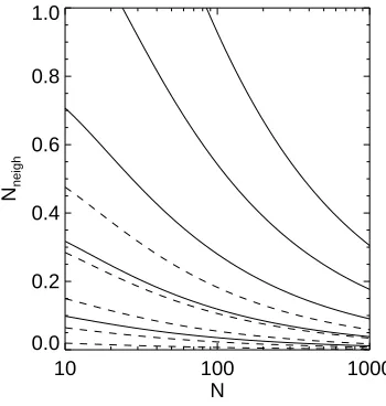
Figure 4. The number of close neighbours to each star (corresponding to the number of (potential) binaries formed per star when Nneigh≪1) as a
func-tion of N, vcritfor Plummer models with RV =0.1 pc. Results are shown
for models with Q=1/2 (solid curves) and Q=3/2 (dashed curves). From bottom to top, both sets of curves represent the results for vcrit=0.10, 0.15,
0.20, 0.25, and 0.30 km s−1.
we assume that a wide binary will form if the relative velocity is smaller than or roughly equal to the orbital velocity of a star in a wide binary system. For two stars with masses M1 and M2in a
circular binary orbit with semi-major axis a, the velocities of the individual stars are given by
v1=M2
r G a(M1+M2)
and v2=v1q−1, (6)
where G is the gravitational constant and q≡M2/M1is the mass
ratio of the binary system. When adopting, for simplicity, q= 1, the above expression reduces to:
vorb≈30 km s−1
M1+M2
M⊙
!−1/2 a
au
−1/2
, (7) where vorbis the velocity of either of the components. In order to be
able to form a binary with semi-major axis a, we require velocity differences to be smaller than the critical velocity
v.2vorb≡vcrit (8)
For our choice of the IMF, the total mass of a binary system is of order 1 M⊙. Binaries with a=3.6×10⁵, 9
×104 and 4
×104 au
thus typically require velocity differences of v.vcrit=0.1, 0.2 and
0.3 km s−1, respectively.
If the velocity distribution of the stars in a given star cluster follows a Maxwell-Boltzmann distribution, then so does also the distribution of relative speeds between the stars. We define the rel-ative velocity,V=vi−vj, with components (Vx,Vy,Vz) and
mag-nitude V =|V|. The distribution over relative speeds is then given by:
fV(V) dV=
1
2√πσ3exp −
V2
4σ2
!
V2dV (9)
(Binney & Tremaine 1987, p. 485), whereσis the one-dimensional velocity dispersion. In the Plummer modelσis given by:
σ2Q=1/2(r)=
16GMcl
18πRV
1+
16r 3πRV
!2
−1/2
(10)
(Heggie & Hut 2003) for a cluster in virial equilibrium (i.e. Q =
1/2). Here, Mclis the total mass of the cluster, and r the distance to
the cluster centre. We can re-write Eq. (10) in units more suitable for the clusters considered in this paper. First, we set Mcl =Nhmi,
where N is the number of stars in the cluster andhmiis their average mass. Using the Kroupa (2001) IMF,hmi=0.55 M⊙. Evaluating the velocity dispersion at the (intrinsic) half-mass radius, r=Rhm≈
0.769RVof the cluster, we find:
σQ=1/2=0.64×
0.1 pc
RV
!1/2 N
100 stars
1/2
km s−1. (11)
The kinetic energy for a star cluster with Q=3/2 is three times that of a cluster with Q=1/2, and therefore the corresponding velocity dispersion is
σQ=3/2= √
3σQ=1/2. (12)
As an example, Fig. 3 shows the distribution of velocities (vx,vy)
for a Plummer model with N = 1000 stars, a virial radius RV =
0.1 pc, and Q =1/2. The distribution of relative speeds between random pairs of stars in the cluster is shown in the right-hand panel. The latter distribution is well approximated by Eq. (9) withσ =
1.9 km s−1, the velocity dispersion at the half-mass radius is given
by Eq. (11).
To find the relative fraction Fb of pairs in a given star
clus-ter which has a relative speed such that they may become bound when the cluster disperses, we integrate Eq. (9) between v=0 and
v=vcrit, where vcritis the critical velocity difference (Eq. 8), below
which we assume that two stars may become bound after cluster dissolution:
Fb =
Rvcrit
0 P(V)dV
R∞
0 P(V)dV
=
Rvcrit
0 exp
−V2 4σ2
V2dV
R∞ 0 exp
−4Vσ22
V2dV , (13)
where we normalised the fraction to unity by dividing by the inte-gral of Eq. (9) between 0 and∞. To find the number of pairs with relative speed less than vcritwe multiply Fbby N−1. Hence:
Nneigh=(N−1) Fb. (14)
If Nneighis smaller than unity one might expect that the binary
frac-tion is proporfrac-tional to Nneigh. In situations where Nneighis larger (i.e.,
larger than unity) and hence many stars are close to each other in velocity space, we might expect to have some competition between the stars to stay bound.
[image:6.612.80.255.311.495.2]10 100 1000 Number of stars 1000
10000
Median semi-major axis (au)
a = 0.1 pc
a = 103
au
10 100 1000
Number of stars 0.00
0.05 0.10 0.15 0.20 0.25 0.30
Wide binary fraction
P2v P2e F2v F2e
0.01 0.10 1.00
Initial virial radius (pc) 1000
10000
Median semi-major axis (au)
a = 0.1 pc
a = 103
au
a = R
0.01 0.10 1.00
Initial virial radius (pc) 0.00
0.05 0.10 0.15 0.20 0.25 0.30
Wide binary fraction
P1v P1e F1v F1e
Figure 5. Monte-Carlo predictions for the dependence of the median semi-major axis a of the escaping wide (103au <a <0.1 pc) binaries (left)
and wide binary fractionB(right) on the number of stars in a cluster (top) and its initial radius R (bottom). Results are shown for Q = 1/2 (solid curves) and Q=3/2 (dashed curves). The thin and thick curves correspond to the Plummer and fractal models, respectively. The diagonal dotted line indicates a=R. The other properties of the modelled clusters are listed in
Table 1.
number of stars, N, in clusters with Q=1/2 and Q=3/2. We show results in the velocity range vcrit=0.1−0.3 km s−1. Depending on
their masses and mass ratios, these velocities correspond to binary systems with semi-major axes from∼ 0.1 pc down to∼104 au.
Velocities of 1.9 km s−1(not shown in Fig. 4) roughly correspond
to binary systems with a=103au.
The values of Nneighin Fig. 4 are rather high, as compared to
wide binary fractions derived in§4.2 and 5, mainly because Nneigh
also contains companion stars outside the separation range 103au −
0.1 pc considered throughout this paper. In addition, we believe that the predicted values will drop further due to the inefficiency of the process. For example, it is not likely (but also not impossible) that two stars with nearly the same velocity will form a wide binary system, if there are other stars in between them. Furthermore, we have only considered the relative velocities, while we have ignored the relative positions between the stars. However, this analysis does provide a strong upper limit on the (wide) binary fractions we might expect after cluster dissolution.
4.2 Upper limits from a Monte-Carlo approach
In the previous section we obtained rough estimates for the number of newly formed binaries using a Maxwellian velocity distribution. However, we were unable to recover the distributions of orbital properties, such as the semi-major axis distribution, and we were not able to take into account the mass spectrum of stars in the clus-ter. We therefore use a somewhat more sophisticated Monte Carlo approach, to obtain estimates for these properties as a function of cluster size, structure, number of stars, and virial ratio, for the mod-els listed in Table 1. Estimates of these properties are obtained us-ing an ensemble of initial condition snapshots of each model.
We identify the potential binaries in each star cluster as
fol-10 100 1000
Number of stars 1000
10000
Median semi-major axis (au)
a = 0.1 pc
a = 103
au
10 100 1000
Number of stars 0.00
0.05 0.10 0.15 0.20 0.25 0.30
Wide binary fraction
P2v P2e F2v F2e
0.01 0.10 1.00
Initial virial radius (pc) 1000
10000
Median semi-major axis (au)
a = 0.1 pc
a = 103
au
a = R
0.01 0.10 1.00
Initial virial radius (pc) 0.00
0.05 0.10 0.15 0.20 0.25 0.30
Wide binary fraction
[image:7.612.40.566.107.322.2]P1v P1e F1v F1e
Figure 6. Same as Fig. 5, but showing the results of the N-body simulations.
lows. For each star with mass M1we determine its nearest
neigh-bour. More precisely, we determine the “most bound” neighbour, i.e., the neighbour with mass M2for which the internal binding
en-ergy
Eb=
1 2
M1M2
M1+M2
v2
−GM1M2
r (15)
is most negative. Here, r is the distance between the two stars, v their velocity difference, and G the gravitational constant. Subse-quently, we select those pairs of stars that are each other’s mutual nearest neighbours, and assume that they will form a binary sys-tem with a semi-major axis of approximately r. Note that not all of these bound pairs may actually form a binary system, as their velocities are perturbed by neighbouring stars. We also ignore the possible presence of triple systems and higher-order systems that may form. The results, shown in Fig. 5, should therefore be con-sidered as a first-order approximation. We will discuss this figure in detail in§5, where we will compare the results with those of
N-body simulations (shown in Fig. 6).
Based on a simple Monte Carlo approach, we find that the wide binary fraction decreases with increasing stellar density, and mildly decreases with increasing virial ratio. However, several sim-plifications have been made, and therefore these results have to be interpreted with care. In particular, we have ignored the interaction of each star with all other stars; we have ignored two-body interac-tions as well as the tidal field of the cluster. In the following section we perform a more accurate analysis to obtain the abundance and properties of wide binaries formed during cluster dissolution, by performing N-body simulations. We will discuss all properties in detail, and compare these to the results obtained using the analyti-cal and Monte-Carlo approaches.
5 RESULTS FROM N-BODY SIMULATIONS
Plummer, Q = 1/2
0.0 0.2 0.4 0.6 0.8 1.0 Mass ratio 0.0
0.2 0.4 0.6 0.8 1.0
Distribution
Plummer, Q = 3/2
0.0 0.2 0.4 0.6 0.8 1.0 Mass ratio 0.0
0.2 0.4 0.6 0.8 1.0
Distribution
Fractal, Q = 1/2
0.0 0.2 0.4 0.6 0.8 1.0 Mass ratio 0.0
0.2 0.4 0.6 0.8 1.0
Distribution
Fractal, Q = 3/2
0.0 0.2 0.4 0.6 0.8 1.0 Mass ratio 0.0
0.2 0.4 0.6 0.8 1.0
[image:8.612.311.558.98.325.2]Distribution
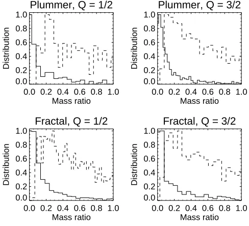
Figure 9. The mass ratio distribution for binary and multiple systems with a>103au resulting from the models in Figs. 7 and 8. The solid and dashed
curves indicate the mass ratio distributions for binaries with M1>1.5 M⊙
and M1<1.5 M⊙, respectively.
In this section we use N-body simulations of evolving star clusters to study how the properties of the newly formed binaries and multiple systems depend on the initial properties of the clus-ters. In §5.1 we describe the orbital properties and multiplicity fractions of wide binaries resulting from a typical star cluster. In
§5.2 we show how the results depend on the initial size R and the number of stars N in clusters consisting of initially single stars, for the models listed in Table 1. In§5.3 we study how the results are affected by the presence of primordial binaries.
5.1 Properties of the newly formed binary population
We perform N-body simulations of Plummer and fractal clusters consisting of N =1000 stars with radii R=0.1 pc (the virial ra-dius for the Plummer models, or the total rara-dius of fractal mod-els), with initial virial ratios Q =1/2 and Q =3/2 (i.e., models P2v, P2e, F2v and F2e in Table 1). Fifty realisations of each model are performed to improve the statistics. The resulting distributions over mass, mass ratio, and semi-major axis for the resulting binary population are shown in Figs. 7 (Plummer models) and 8 (fractal models).
The left-hand panels in Figs. 7 and 8 show the separation distribution f (a) of the resulting binary population. Note that bina-ries of all separations are included in these figures, irrespective of whether they are actually able to survive in the Galactic field or not. The figures illustrate that the separation distribution of the newly formed binaries is bimodal, and consists of a small-separation
dy-namical peak and a large-separation dissolution peak. The tighter
binaries in the dynamical peak are formed during dynamical en-counters in the cluster, and most of them remain mutually bound during the further evolution of the cluster. The wide binaries in the
dissolution peak, on the other hand, are formed during the
dissolu-tion phase of star clusters.
The two sets of models with a Plummer density distribution result in a small dynamical peak, indicating that dynamical
inter-Plummer, Q = 1/2
0.0 0.2 0.4 0.6 0.8 1.0 Eccentricity 0.0
0.2 0.4 0.6 0.8 1.0
Distribution
Plummer, Q = 3/2
0.0 0.2 0.4 0.6 0.8 1.0 Eccentricity 0.0
0.2 0.4 0.6 0.8 1.0
Distribution
Fractal, Q = 1/2
0.0 0.2 0.4 0.6 0.8 1.0 Eccentricity 0.0
0.2 0.4 0.6 0.8 1.0
Distribution
Fractal, Q = 3/2
0.0 0.2 0.4 0.6 0.8 1.0 Eccentricity 0.0
0.2 0.4 0.6 0.8 1.0
Distribution
Figure 10. The eccentricity distribution f (e) for binary and multiple sys-tems with a>103au resulting from the models in Figs. 7 and 8. The
his-tograms indicate f (e), while the curves show the corresponding cumulative distributions. The filled circles represent the cumulative thermal eccentric-ity distribution f (e)=2e.
actions during the lifetime of the cluster generally do not result in the formation of close binaries. This is not surprising, as all stars in the Plummer models are initially given random velocities. Due to the immediate expansion of the Plummer model with Q=3/2, the
dynamical peak is completely absent in this case.
For the models with a fractal density distribution in Fig. 8, there are numerous binaries in the dynamical peak. The fact that the dynamical peak is stronger for models F2v/F2e than for models P2v/P2e is due to both the initial positions and the initial veloc-ities being correlated in the fractal models. Although the average distance between two random stars is similar for both models, the average distance between nearest neighbours in the fractal mod-els is smaller (as they are clumpy). As nearby stars in the clumpy structure also have similar velocities, frequent dynamical interac-tions occur, resulting in a strong dynamical peak.
For our choice of initial conditions, binaries in the
dynami-cal peak have separations in the range 1−103 au, with a median
value near 50−100 au. The median value is set by the typical dis-tance between stars in the most densely populated regions of the cluster during the formation of these binary systems. Interestingly, this also corresponds to the observed peak in the Taurus-Auriga bi-nary separation distribution (e.g., Leinert et al. 1993; Kroupa et al. 1999).
Binaries in the dissolution peak have a semi-major axis in the separation range 103au
−5 pc. The widest binaries in the dissolution
peak will immediately break up in the Galactic field, hence our
choice to study the wide binary population in the separation range 103 au
−0.1 pc throughout this paper. The median separation of binaries in the dissolution peak occurs at a≈0.1−0.2 pc. As we will see later (§5.2.2), this value is set by the initial size of the cluster.
For practical purposes, we consider three ranges in semi-major axis: close binaries with a < 103 au, wide binaries with
[image:8.612.54.298.102.324.2]Q = 1/2
100 101
102 103
104 105
106 Semi-major axis (AU) 0.0
0.2 0.4 0.6 0.8 1.0
Semi-major axis distribution
100 101
102 103
104 105
106 Semi-major axis (AU) 0.0
0.2 0.4 0.6 0.8 1.0
Mass ratio
0.1 1.0 10.0
M1 (Msun) 0.0
0.2 0.4 0.6 0.8 1.0
Mass ratio
Q = 3/2
100 101
102 103
104 105
106 Semi-major axis (AU) 0.0
0.2 0.4 0.6 0.8 1.0
Semi-major axis distribution
100 101
102 103
104 105
106 Semi-major axis (AU) 0.0
0.2 0.4 0.6 0.8 1.0
Mass ratio
0.1 1.0 10.0
M1 (Msun) 0.0
0.2 0.4 0.6 0.8 1.0
[image:9.612.60.541.107.402.2]Mass ratio
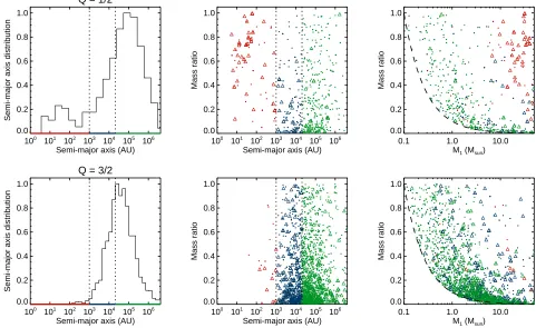
Figure 7. The semi-major axis distribution (left), the correlation between mass ratio q and semi-major axis a (middle) and between primary mass and mass ratio (right). The histograms in the semi-major axis distribution are normalized such that the maximum value equals unity. The properties of the orbits of binary systems and higher-order multiple systems are indicated with the dots and triangles, respectively. For each multiple system with n stellar components, we have included all n−1 orbits. Results are shown for 50 Plummer models with N=1000 and R=0.1 pc, and virial ratios of Q=1/2 (top) and Q=3/2 (bottom). The vertical dashed lines indicate a=103au and a=0.1 pc, respectively. The dashed curve in the right-hand panel indicates the minimum mass
ratio qmin(M1)=Mmin/M1.
Table 2. The specific binary fractionBfor the models shown in Figs. 7 and 8, in which the three ranges in semi-major axis are divided with the vertical dotted lines.
Model B B B
Separation range <103au 103au−0.1 pc >0.1 pc
P2v (N=1000) 0.2% 0.3% 0.8%
P2e (N=1000) 0.1% 1.4% 2.8%
F2v (N=1000) 3.3% 1.8% 2.6%
F2e (N=1000) 2.2% 0.6% 1.1%
The limits are indicated with the vertical dotted lines in the figures. Most close binaries that are found in star clusters are formed via the “normal” star formation process, with the small number seen in these simulations formed by dynamical interactions. The wide and extremely wide binaries are formed during the cluster dissolution phase. Note however, that the vast majority of the extremely wide binaries are unstable in the Galactic field, and are ionised quickly after their formation.
For the models in Figs. 7 and 8, the specific binary fraction (i.e., the fraction of binary systems in a certain semi-major axis range) of the three types of binaries are listed in Table 2. The high-est wide binary fractions of a few per cent (in the separation range 103 au
−0.1 pc) are obtained for Plummer models with Q =3/2, and fractal models with Q=1/2.
The middle and right-hand panels of Figs. 7 and 8 show the correlations between semi-major axis, mass ratio, and primary mass, for the binary and multiple (higher-order) systems in each of the models. The panels indicate the presence of a large num-ber of newly formed multiple systems. These higher-order systems are stable in isolation, but a large fraction will not be able to sur-vive in the Galactic field, where tidal forces will rapidly remove the outer component from the system. Figs. 7 and 8 therefore overes-timate the fraction of higher-order multiple systems. Note, in par-ticular, the high prevalence of multiple systems in the dynamical
peak. Many outer components of these systems fall in the dissolu-tion peak. These systems are therefore wide higher-order systems.
For the Plummer models, the dynamical peak consists of sys-tems with high masses and high mass ratios. This is a well-known signature of mass segregation: the highest-mass stars sink to the cluster centre, where they form close binaries (e.g. Heggie & Hut 2003). During the dissolution phase of the clusters, these close, massive binaries act like single stars when forming a “wide bi-nary”, which is in fact a wide triple or higher-order multiple system. The effect of mass segregation is less visible for the fractal models, where dynamical interactions in the subclumps play a greater role. However, Fig. 8 still clearly shows that most massive systems are mostly close (a < 103 au) and often higher-order. In addition to
[image:9.612.43.249.534.611.2]Q = 1/2
100 101
102 103
104 105
106 Semi-major axis (AU) 0.0
0.2 0.4 0.6 0.8 1.0
Semi-major axis distribution
100 101
102 103
104 105
106 Semi-major axis (AU) 0.0
0.2 0.4 0.6 0.8 1.0
Mass ratio
0.1 1.0 10.0
M1 (Msun) 0.0
0.2 0.4 0.6 0.8 1.0
Mass ratio
Q = 3/2
100 101
102 103
104 105
106 Semi-major axis (AU) 0.0
0.2 0.4 0.6 0.8 1.0
Semi-major axis distribution
100 101
102 103
104 105
106 Semi-major axis (AU) 0.0
0.2 0.4 0.6 0.8 1.0
Mass ratio
0.1 1.0 10.0
M1 (Msun) 0.0
0.2 0.4 0.6 0.8 1.0
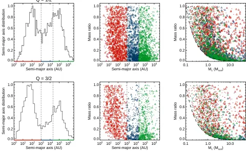
[image:10.612.60.540.107.402.2]Mass ratio
Figure 8. Same as Fig. 7, but now for fractal models with N=1000 and R=0.1 pc , and virial ratios of Q=1/2 (top) and Q=3/2 (bottom); in each case fifty realisations have been simulated.
The correlations between the primary mass and mass ratio dis-tributions for the binary and multiple systems are similar to those expected from random pairing of individual stars. To first order ap-proximation, the masses of the two stars, M1and M2, in each binary
are uncorrelated; one would therefore expect something similar to random pairing (e.g., Kouwenhoven et al. 2009), where the aver-age mass ratio decreases with increasing binary system mass. The resulting mass ratio distributions for binary and multiple systems with a >103au (i.e., those in the dissolution peak) are shown in
Fig. 9, which illustrates the dependence of the mass ratio distribu-tion on mass.
Based on the analysis of a sample of 798 common proper mo-tion pairs, Trimble (1987) also come to the conclusion that the very wide binary population in the field is consistent with random pair-ing, and Valtonen (1997) come to the same conclusion from their simulations of three-body encounters. However, the wide binary population does not result from random pairing alone, as the in-teraction between two stars depends on their mutual gravitational attraction, and the probability of two stars forming a binary is thus proportional to the product M1M2. In other words, gravitational
fo-cusing (e.g., Gaburov et al. 2008) plays an important role. Measurements of the eccentricity distribution of wide binaries are currently unavailable, due to the large orbital periods and in-completeness. If we suspect that the vast majority of wide binaries probably have formed dynamically, and as dynamical interactions are common among the widest binaries (with respect to closer-in binaries), the best guess is perhaps the thermal eccentricity distri-bution f (e)=2e (06e<1) (Heggie 1975, see also Kroupa 2008 for a derivation), which results from energy equipartition. The ec-centricity distributions resulting for binaries in the dissolution peak
(a>103au) are shown in Fig. 10. As expected, the thermal
eccen-tricity distribution is a good approximation for the newly formed binary population.
If wide binaries form during the dissolution process of a star cluster, then the orbital and spin angular momenta of the compo-nents should be randomly aligned. On the other hand, if the two components formed together in some way it might be that the or-bital and spin angular momenta of the components will be corre-lated (as seen for example in the observations of∼100-au Ae/Be binaries by Baines et al. 2006). Therefore, observations of the rela-tive alignments of orbital and spin angular momenta could provide constraints on the possible formation mechanisms of very wide bi-naries.
Finally, the age difference (between primary and companion star) for a population of wide binaries could provide a clue to their origin (see, e.g., Kraus & Hillenbrand 2009a). For a star clus-ter with a certain age spread, one might expect the components of the resulting wide binary population to exhibit a similar age difference. This age difference is measurable, but only for young (.10 Myr) binary systems. On the other hand, this age difference may be smaller than expected from random pairing, if an initial correlation between position and velocity exists.
5.2 Dependence on cluster properties
cluster properties listed in Table 1. We compare the results that we derived earlier using Monte Carlo simulations (Fig. 5), with the re-sults of N-body simulations, shown in Fig. 6.
5.2.1 Dependence on the initial cluster mass
The top panels of Fig. 6 show the median semi-major axis amedand
the binary fractionBof wide binaries (103au<a<0.1 pc) as a
function of the number of stars N in a cluster. For both the Plummer models and the fractal models, ameddoes not vary significantly with
N and the virial ratio Q. The reason for this is that all these models
have an identical size R. Since R is the most important size scale
imposed on the modelled star clusters, it determines the size scaling (i.e., semi-major axis distribution) of the newly formed binaries.
The dependence ofBon N and Q is qualitatively the same as the analytical predictions shown in Fig. 4 and the Monte Carlo ap-proximation shown in Fig. 5 . The wide binary fractionBdecreases with increasing N because the stars are further apart in velocity space (cf. Fig. 3), i.e., the velocity dispersion is larger, and hence two neighbouring stars are less likely to form a bound system.
For the N-body simulations we find that the fractal model with
Q=1/2 provides the highest wide binary fractions, although the difference between models is fairly small (especially when com-pared to the difference with increasing N). Models with Q =3/2 generally result in a smaller wide binary fraction than those with
Q=1/2, due to the larger distance between the stars in velocity space (see Eqs. 11 and 12). The curves for the fractal models in Figs. 5 and Fig. 6 are almost the same, indicating that the Monte Carlo approach provides a good estimate of the wide binary popu-lation. For the Plummer models, the Monte Carlo approach predicts a binary fraction that is too high, which is due to the fact that the positions and velocities of stars in the Plummer models as we ini-tialise them are uncorrelated.
5.2.2 Dependence on the initial cluster size
The bottom panels of Fig 6 shows the dependence of amedandB
on the initial size R of the clusters. Again, these values are only for
wide binaries with 103 au<a<0.1 pc. Note the different
defini-tions of R: for the Plummer models R represents the virial radius, while for the fractal models R represents the radius of the sphere enclosing the whole system. Note again the similarity between the Monte Carlo approximation shown in Fig. 5 and the N-body mod-els.
As discussed above, the initial cluster size R determines the length scale in each model, and therefore the size scaling of the semi-major axis distribution of the newly formed binaries. For ex-ample, changing the initial size of the clusters shown in Figs. 7 and 8 would simply result in the semi-major axis distribution in the left-hand panels being shifted to smaller or larger values of a.
This direct dependence of f (a) on R is not seen directly in Fig. 5 because we only show the results for wide binaries in the separation range 103au<a<0.1 pc, and because f (a) is bimodal.
However, the R-dependent median semi-major axis and binary frac-tion can be explained by the dynamical peak and dissolufrac-tion peak shifting through the range 103au<a<0.1 pc whilst varying R.
The highestBis found when either the dynamical peak, or the
dissolution peak, is centred in the separation range 103 au<a<
0.1 pc. For our choice of the initial conditions, this peak occurs at
R=0.025 pc for the Plummer models, when the dissolution peak is centred in the range 103au−0.1 pc. The peak inBoccurs at R≈
0.0 0.2 0.4 0.6 0.8 1.0 Primordial binary fraction 1000
10000
Median semi-major axis (au)
a = 0.1 pc
a = 103 au
0.0 0.2 0.4 0.6 0.8 1.0 Primordial binary fraction 0.00
0.05 0.10 0.15 0.20 0.25 0.30
Wide binary fraction
B = B0
0.1 1.0 10.0 100.01000.0 Primordial semi-major axis (au) 1000
10000
Median semi-major axis (au)
a = 0.1 pc
a = 103 au
0.1 1.0 10.0 100.01000.0 Primordial semi-major axis (au) 0.00
0.05 0.10 0.15 0.20 0.25 0.30
[image:11.612.307.536.109.299.2]Wide binary fraction
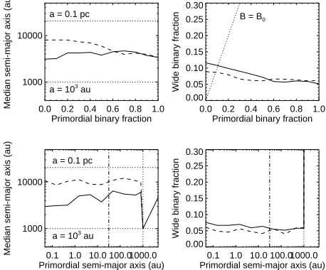
Figure 11. The effect of primordial binarity on the formation of wide bi-naries, for Plummer models with N =10 and R=0.1 pc. The solid and dashed curves in each panel indicate the results for Q=1/2 and Q=3/2, respectively. Top: the effect of a variable primordial binary fractionB0. The
bottom horizontal dotted line indicates a=18.2 au, the median semi-major axis for primordial binaries. Bottom: the effect of the semi-major axis a0for
models with a primordial binary frequencyB0=50% in which each binary
has a semi-major axis a=a0. The dash-dotted lines indicate a=18.2 au, the median semi-major axis of binary systems in the Galactic field. The ver-tical dotted line indicates a=103au, beyond which all primordial binaries are classified as wide binaries.
0.15 pc for the fractal models with Q=1/2 and at R≈0.6 pc for fractal models with Q=3/2, when the dynamical peak is centred in the range 103au
−0.1 pc.
Given our set of initial conditions, compact clusters result in a wide binary fraction of 8−12%, irrespective of virial ratio and mor-phology. For more extended clusters, those with a Plummer struc-ture and those with a higher virial ratio result in a smaller binary fraction. The difference between the Plummer and fractal models can be explained by (i) the difference in the definition of R for the two sets of models, and (ii) by the different intrinsic separation dis-tribution (see the left-hand panels in Figs. 7 and 8).
The cluster size R determines the length scale of the system, and therefore determines the typical semi-major axis of the newly formed wide binaries. Other, less important length scales in the sys-tem are the mean distance between two stars, which depends on the parameters R, N, and the stellar density distribution (see§5.2.1), as well as the typical semi-major axis of primordial binary systems (see§5.3).
5.3 Effects of primordial binarity
In the analysis above we have considered star clusters that initially consist of single stars only. The results for star clusters with a non-zero primordial binary fraction are very similar to the results de-scribed above, with the difference that the components of the wide “binary” are now in many cases primordial binaries. In other words, the majority of the wide “binaries” that formed in the simulations described in the previous sections, actually describe the outer orbits of wide triple and quadruple systems.
listed in Table 1, but now we include a non-zero primordial binary fraction. We perform the simulations with primordial binary frac-tionsB0 ranging from 0% to 100%. We adopt the Kroupa (1995)
birth period distribution. This distribution is derived from a detailed analysis of observed stellar populations, and has the form
fP(P)=2.5
log P−log Pmin
45+ log P−log Pmin2
(16)
for Pmin6P6Pmax, where log Pmin =1, log Pmax =8.43, and P
is the period in days. We adopt a thermal eccentricity distribution
f (e)=2e (06e<1). We adopt a flat mass ratio distribution f (q)=
1 with 0<q≡M2/M1 <1 (i.e., we apply pairing function PCP-I;
see Kouwenhoven et al. 2009). Subsequently, we generate an initial population from this birth population, by applying eigenevolution as described in Kroupa (1995). All binaries are assigned random orientations and orbital phases at the beginning of the simulations. Due to the inclusion of binary components, the total mass of each cluster increases slightly (up to a maximum of 50% for a pri-mordial binary fraction of 100%), although the number of “sys-tems”, N=S+B remains constant. Strictly speaking, it is thus not
appropriate to directly compare clusters with and without binaries, as we have changed more than one parameter: binarity and clus-ter mass (see, e.g., Kouwenhoven & de Grijs 2008). However, as the increase in cluster mass due to adding the companions is rather small, we will ignore this issue.
The results for clusters with a varying primordial binary frac-tionB0 is shown in the top panels of Fig. 11. For small binary
fractions, the results are very similar to those of clusters without primordial binaries. The properties of the resulting wide binary population depend mildly on Q. An increasing Q results in, on av-erage, wider binaries, hence in a larger fraction of binaries with
a > 0.1 pc, and therefore in a slightly smaller wide binary frac-tion. Note thatBdecreases slightly with increasingB0. A larger
primordial binary fraction results in a smaller wide binary fraction, possibly because of the destruction of newly formed wide binaries by primordial binaries (which have a significantly larger collisional cross-section than single stars).
Whether or not primordial binarity affects the formation of wide binaries depends not only on the primordial binary fraction, but also on the properties of these binaries: the semi-major axis (or period) distribution, the eccentricity distribution and the mass ratio distribution. The most important of these is the semi-major axis distribution f (a), as it determines the internal binding energy of a binary and the cross-section for gravitational interactions between binaries and other binaries or single stars. In order to extract the dependence on f (a), we simulate clusters in which all binaries have a single value for a=a0. We vary a0in each cluster, and determine
the number of newly-formed binaries. In all simulations we adopt a primordial binary fraction of 50%, a flat mass ratio distribution and a thermal eccentricity distribution.
The results of these simulations are shown in the bottom pan-els of Fig. 11. For modpan-els with a0 <103au, most primordial
bina-ries survive, while additional wide binary, triple, and quadruple sys-tems are formed. In fact, the resulting wide binary fraction is practi-cally independent of the primordial binary fractionB0. For models
with a0 > 103 au, all primordial binary systems are classified as
wide binaries. For these models we therefore haveB ≈ B0and a
median semi-major axis equal to a0, which results in the glitches at
a=103au in Fig. 11.
The wide orbits are part of systems with 2, 3, and 4 compo-nents. They are formed by randomly pairing single stars and pri-mordial binary systems together. The number of multiple systems
of each degree can thus be estimated by simply calculating the probability of randomly drawing a single-single, single-binary, and binary-binary pair. When assuming a primordial binary fractionB0,
the multiplicity distribution of the resulting wide population can be estimated as follows:
Wide binary fraction= B(1− B0)2 (17)
Wide triple fraction= 2BB0(1− B0) (18)
Wide quadruple fraction= BB2
0, (19)
where we have made the assumption that none of the primordial binary systems has broken up.
All models shown in Fig. 11 result in wide binary fractions
B ≈8% that are more or less independent ofB0and a0. The value
ofBis therefore primarily determined by the initial values of the number of system N in the cluster, and its initial size R.
If we assume that the wide orbits in the bottom panels of Fig. 11 (whereB0 = 50%) are formed of randomly paired
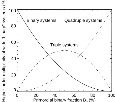
com-ponents (i.e., single stars or primordial binaries), we can calculate the fraction of higher-order multiple systems among theB=8% wide binaries. Among these, we predict that 25%, 50%, and 25%, are binary, triple, and quadruple systems, respectively. In this exam-ple, we thus expect 75% of the “wide binaries” to be higher-order multiple systems. Due to the random process, the outer orbits of these systems are expected to be uncorrelated with the inner orbits or stellar spin axes.
The ratios between wide binary, triple, and quadruple systems are therefore indicative ofB0. A survey for higher-order
multiplic-ity among “wide binary systems” can thus be used to constrain the primordial binary fraction. Given the fact that the majority of stars do form in binary systems, we predict a very high fraction of higher-order multiple systems among wide “binary” systems; see Fig. 12. Our proposed mechanism could explain the existence of the observed wide multiple systems (Mamajek et al. 2009), and our predictions are strongly supported by the surveys of Makarov et al. (2008) and Faherty et al. (2010), who find that a high fraction of the common proper motion pairs in their survey contain inner binary or triple systems, which is significantly higher than in populations of other types of binaries.
6 SUMMARY AND DISCUSSION
Observations have shown that∼ 15% of binaries are wide (a >
103 au). These wide binaries are difficult to explain as being the
result of star formation as it is difficult to see how wide binaries can form (especially those>104 au), and they would be rapidly
destroyed in clustered star forming environments. Whilst 10 – 30% of stars do appear to form in an ‘isolated’ environment in which such binaries could possibly survive, in order to explain the fraction of wide binaries, almost all stars forming in isolated environments would have to form wide binaries. Further, such wide binaries can-not be formed later in any significant numbers by dynamical inter-actions in the Galactic field.
In this paper we study the possibility of wide binary formation during the dissolution phase of star clusters, in particular, during the rapid expansion of clusters after gas expulsion. We study this pos-sibility using (1) an analytical approach in an idealised situation, (2) a Monte Carlo approach, and (3) detailed N-body simulations. Our main conclusions are as follows: