Compact approximation stencils based on integrated radial basis functions for fluid flows

(1)

UNIVERSITY OF SOUTHERN QUEENSLAND

COMPACT APPROXIMATION STENCILS

BASED ON INTEGRATED RADIAL BASIS

FUNCTIONS FOR FLUID FLOWS

A dissertation submitted by

THUY-TRAM HOANG-TRIEU

B.Eng., (Hon.), Tomsk Polytechnic University, Russia, 2008

Engineer, (Hon.), Tomsk Polytechnic University, Russia, 2009

For the award of the degree of

Doctor of Philosophy

(2)

(3)

Dedication

(4)

Certification of Dissertation

I certify that the idea, experimental work, results and analyses, software and conclusions reported in this dissertation are entirely my own effort, except where otherwise acknowledged. I also certify that the work is original and has not been previously submitted for any other award.

Thuy-Tram HOANG-TRIEU Date

ENDORSEMENT

Prof. Nam MAI–DUY, Principal supervisor Date

Dr. Canh–Dung TRAN, Co-supervisor Date

(5)

Acknowledgements

It would not have been possible to write this thesis without the help and support of the kind people around me.

Above all, I would like to express my special appreciation and thanks to my supervisors, Prof. Nam Mai-Duy, Dr. Canh-Dung Tran and Prof. Thanh Tran-Cong, for their insightful guidance and indispensable suggestions. I am deeply grateful for their helps and their patience over the past years.

I would like to acknowledge the University of Southern Queensland (USQ) for the PhD Scholarship and the Computational Engineering and Science Research Centre (CESRC) for the financial supplement.

I would like to thank Dr. Lan Mai-Cao for introducing me to an opportunity to study at CESRC, USQ.

I would also like to thank my friends for their encouragement over the past years.

(6)

Abstract

This research project is concerned with the development of compact local inte-grated radial basis function (CLIRBF) stencils and its verification in the simula-tion of Newtonian and non-Newtonian fluid flows governed by the streamfuncsimula-tion- streamfunction-vorticity formulation. In the CLIRBF stencils, nodal values of the governing equations at selected nodes on a stencil are also incorporated into the IRBF ap-proximations with the help of integration constants to enhance their accuracy. The proposed CLIRBF stencils overcome some of the weaknesses of the local RBF stencils (low order accuracy) and the global RBF approximations (full sys-tem matrices).

Four main research tasks are carried out

• Development of CLIRBF stencils for approximating the field variables and their derivatives.

• Incorporation of CLIRBF stencils into two formulations for discretisation of ordinary/partial differential equation (ODEs/PDEs), namely point col-location and subregion colcol-location.

• Discretisation of fourth-order elliptic ODEs/PDEs, sets of two second-order PDEs representing fourth-order PDEs, and second-order ODEs/PDEs.

• Discretisation of transient problems, where time derivatives are approxi-mated using the Crank-Nicolson/Adams Bashforth scheme.

The proposed CLIRBF stencils are verified in a wide range of problems: (i) ODEs/PDEs with analytic solutions; (ii) heat transfer problems; (iii) Newto-nian fluid flows (Burger’s equations, lid-driven cavity flows, natural convection in rectangular and nonrectangular domains); and viscoelastic fluid flows (Poiseuille flows and corrugated tube flows of Oldroyd-B fluid).

(7)

Papers resulting from the Research

Journal papers

1. Hoang-Trieu, T.-T., Mai-Duy, N., and Tran-Cong, T. (2011). Compact local stencils employed with Integrated RBFs for fourth-order differential problems. SL: Structural Longevity, 6(2):93–108

2. Hoang-Trieu, T.-T., Mai-Duy, N., and Tran-Cong, T. (2012). Several com-pact local stencils based on Integrated RBFs for fourth-order ODEs and PDEs. CMES Computer Modeling in Engineering and Sciences, 84(2):171– 203.

3. Hoang-Trieu, T.-T., Mai-Duy, N.,Tran, C. -D., and Tran-Cong, T. (2013). A finite-volume method based on compact local integrated radial basis func-tion approximafunc-tions for second-order differential problems. CMES

Com-puter Modeling in Engineering and Sciences, 91(6):485–516.

4. Pham-Sy, N., Tran, C. -D., Hoang-Trieu, T.-T., Mai-Duy, N., and Tran-Cong, T. (2013). Compact local IRBF and domain decomposition method for solving PDEs using a distributed termination detection based parallel al-gorithm. CMES Computer Modeling in Engineering and Sciences, 92(1):1– 31.

5. Mai-Duy, N., Thai-Quang, N., Hoang-Trieu, T.-T., and Tran-Cong, T. (2013). A compact 9 point stencil based on integrated RBFs for the convection-diffusion equation. Applied Mathematical Modelling, 235:302–321.

6. Hoang-Trieu, T.-T., Mai-Duy, N.,Tran, C. -D., and Tran-Cong, T. Compact local IRBF stencils for viscoelastic fluid flows. (to be submitted).

7. Hoang-Trieu, T.-T., Mai-Duy, N.,Tran, C. -D., and Tran-Cong, T. Compact local IRBF stencils for transient problems. (to be submitted).

Conference papers

1. Hoang-Trieu, T.-T., Mai-Duy, N., Tran, C.-D., and Tran-Cong, T. (2012). Compact local integrated RBF stencil based on finite volume formulation for second-order differential problems. 4th International Conference on

(8)

Papers resulting from the Research vi

2. Pham-Sy, N., Tran, C. -D., Hoang-Trieu, T.-T., Mai-Duy, N., and Tran-Cong, T. (2012) Development of parallel algorithm for boundary value problems using compact local integrated RBFN and domain decomposition.

4th International Conference on Computational Methods (ICCM 2012),

(9)

Acronyms and Abbreviations

BEM Boundary Element Method

CDS Central Difference Scheme

CFD Computational Fluid Dynamics

CLIRBF Compact Local Integrated Radial Basis Function

CLIRBF-FVM Compact Local Integrated Radial Basis Function-FiniteVolume Method

CLIRBF-PCM Compact Local Integrated Radial Basis Function-Point Col-location Method

CLS Compact Local Stencil

CM Convergence measure

DQM Differential Quadrature Method

DRBF Differential Radial Basis Function

FD Finite Difference

FDM Finite Difference Method

FEM Finite Element Method

FVM Finite Volume Method

GE Governing Equation

IRBF Integrated Radial Basis Function

MQ Multiquadric

ODE Ordinary Differential Equation

PDE Partial Differential Equation

RBF Radial Basis Function

RBFN Radial Basis Function Network

SCHOS Single Cell High Order Scheme

SD Spectral Difference

(13)

Acronyms and Abbreviations xi

UCM Upper-Convected Maxwell

UDS Upwind Difference Scheme

(14)

List of Tables

2.1 ODE, 5-node CLS, 3-node CLS with GE and 3-node CLS without GE: RelativeL2 errors of the solutionuusing some fixed and the optimal values of β for three grids. . . 31 2.2 PDE, Example 1,5_×5-node CLS: Condition numbers of the

sys-tem matrixA and relativeL2 errors of the solution uusing a fixed value and the optimal value of β for several grids. . . 32 2.3 PDE, Example 1, 3_×3-node CLS: relative L2 errors of the

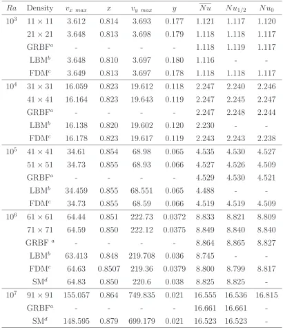
solu-tion u for several grids. . . 35 2.4 PDE, Example 2,Re= 100,β = 20: Extreme values of the velocity

profiles on the centerlines by the proposed method and several other methods. It is noted that N is the polynomial degree. . . . 37 2.5 PDE, Example 2, Re = 1000, β = 20: Extreme values of the

velocity profiles on the centerlines by the proposed method and several other methods. It is noted that N is the polynomial degree. 38

3.1 Example 1, R = 40, β = 2.5: Maximum relative errors and rates of convergence by the original local IRBF and present compact local IRBF methods. The rate presented here is the exponent of

O(hrate) that is computed over two successive grids (point-wise)

and also over the whole set of grids used. LCR stands for local convergence rate. . . 52 3.2 Example 1, R = 40, β = 0.9: Maximum relative errors and rates

of convergence by the original local IRBF and present compact local IRBF methods. The rate presented here is the exponent of

O(hrate) that is computed over two successive grids (point-wise)

and also over the whole set of grids used. . . 52 3.3 Example 1: Maximum relative errors at a grid size ofh= 1/32.

Re-sults by UDS, CDS and SCHOS are extracted from (Gupta et al., 1984). . . 53 3.4 Natural convection: Grid convergence study. “Benchmark” and

“Benchmark*” refer to the finite difference and pseudo spectral results in (Davis, 1983) and (Quere, 1991), respectively. . . 57 3.5 Natural convection: Condition numbers of the conversion matrix

for the vorticity equation (middle column) and the energy equa-tion (last column) which are measured when the Picard iteraequa-tion scheme has achieved convergence. . . 58 3.6 Lid-driven cavity flow: Grid convergence study for extreme values

(15)

List of Tables xiii

3.7 Lid-driven cavity flow: Grid convergence study for features of the primary vortex. “Benchmark” and “Benchmark*” refer to the fi-nite difference and pseudo spectral results in (Ghia et al., 1982) and (Botella and Peyret, 1998), respectively. . . 62

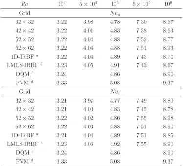
4.1 Natural convection in a square slot: Maximum velocities on the middle planes and the average Nusselt number by the present CLIRBF-FVM (3 Gauss points) and by some other methods. . . . 86 4.2 Natural convection in an annulus defined by concentric outer square

and inner circular cylinders: the average Nusselt number on the outer (Nuo) and inner (Nui) cylinders by the present CLIRBF-FVM (1 Gauss point) and by some other methods (RBF, CLIRBF-FVM and DQM). . . 88

5.1 Planar Poiseuille flow of Newtonian fluid: RMS errors of the com-puted solutions for several values of Re. . . 98 5.2 Planar Poiseuille flow of Oldroyd-B fluid, grid of 21_×21: RMS

errors of the computed solutions for several values of W e. . . 99 5.3 Planar Poiseuille flow of Oldroyd-B fluid, W e = 9: Grid

conver-gence study. . . 99 5.4 Circular Poiseuille flow of Newtonian fluid: RMS errors of the

computed solutions for Re=_{10,109_}_{. . . 101} 5.5 Circular Poiseuille flow of Oldroyd-B fluid, grid of 21_×21: RMS

errors of the computed solutions for several W e numbers. . . 102 5.6 Circular Poiseuille flow of Oldroyd-B fluid, W e = 9: Grid

conver-gence study. . . 102 5.7 Corrugated tube flow of Newtonian fluid, Re= 0: Computed flow

resistances. . . 106 5.8 Corrugated tube flow of Newtonian fluid,ε = 0.3,M = 0.16: Flow

resistances for a wide range of Re. . . 107 5.9 Corrugated tube flow of Oldroyd-B fluid, ǫ = 0.1, M = 0.5:

Com-puted flow resistances. . . 109

6.1 Example 2, Hyperbolic equation, N = 42, ∆t = 10−4_{, the root} mean squared errors at several time levels t. . . 120 6.2 Example 3. Exact solution . . . 123 6.3 Example 3. Solution by CLIRBF . . . 123 6.4 Example 4, Problem 1, Re = 100, t = 0.01, ∆t = 10−4_, _N ₌

21_×21. Comparison of absolute errors foruandv at several mesh points. . . 126 6.5 Example 4, Problem 1,Re= 100,t = 0.5, ∆t= 10−2_,_N _{= 21}_×_21.:

(16)

List of Figures

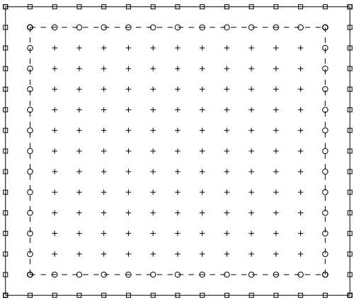
2.1 A problem domain and a typical discretisation. Legends square, circle and plus are used to denote the boundary nodes, the inte-rior nodes next to the boundary and the remaining inteinte-rior nodes, respectively. . . 21 2.2 A schematic representation of the proposed 5_×5-node stencil

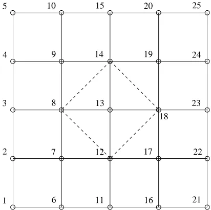
as-sociated with node (i, j). Over the stencil, nodes are locally num-bered for bottom to top and left to right, where 13_≡(i, j). Nodal values of the governing equation used as extra information are placed on a diamond shape. . . 22 2.3 A schematic representation of the proposed 13-node stencil

associ-ated with node (i, j). Over the stencil, nodes are locally numbered for bottom to top and left to right, where 7_≡ (i, j). Nodal values of the governing equation used as extra information are placed on a diamond shape. . . 25 2.4 ODE: Relative L2 errors of the solution u and condition numbers

of the system matrix against the grid size by the proposed stencils and the standard local IRBF one. It is noted that we employ

β = 24 for local and compact local 5-node stencils, β = 34 for 3-node CLS without GE, and β = 5.6 for 3-node CLS with GE. . . 29 2.5 ODE, 5-node CLS, β = 24: The solution accuracy and matrix

condition number against the grid size by Implementation 1 and Implementation 2. . . 30 2.6 PDE , Example 1,13-node CLS, β = 18: The solution accuracy

and matrix condition number against the grid size. Results by the FD 13-node stencil are also included. . . 33 2.7 PDE, Example 1, 13-node CLS, β = 18: The solution accuracy

and matrix condition number against the grid size by Implemen-tation 1 and ImplemenImplemen-tation 2. . . 34 2.8 PDE, Example 2, Re = 1000: Profiles of the x₋component of

the velocity vector along the vertical centerline for several grids. Results by the FDM (Ghia et al., 1982) are also included. . . 36 2.9 PDE, Example 2, Re = 1000: Profiles of the y₋component of

the velocity vector along the horizontal centerline for several grids. Results by the FDM (Ghia et al., 1982) are also included. . . 37 2.10 PDE, Example 2, 3_×3-node CLS, a grid of 111_×111:

Stream-lines of the flow at several Reynolds numbers. It can be seen that secondary vortices are clearly captured. . . 39 2.11 PDE, Example 2,3_×3-node CLS, a grid of 111_×111: Iso-vorticity

(17)

List of Figures xv

3.1 Example 1, rectangular domain: exact solutions at several values of R. . . 49

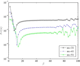
3.2 Example 1, rectangular domain: the maximum relative error against the RBF width (β =a/h) at a grid of 33_×33. The optimal value of β is a decreasing function of R. . . 50

3.3 Example 1, rectangular domain: the maximum relative error against the RBF width (β =a/h) at a grid of 33_×33. The optimal value of β is a decreasing function of R. . . 51

3.4 Example 2, non-rectangular domain: The exact solution (left) and the grid-convergence behaviour of the proposed stencil (right) for

R = 1 (top), R = 10 (middle) and R = 25 (bottom). Grids em-ployed are (10_×10,20_×20,_{· · ·},150_×150). The solution converges apparently asO(h4.24_{) for} _R_{= 1,} _O₍_h3.60_{) for} _R _{= 10 and}_O₍_h3.36₎ for R= 25. . . 54

3.5 Natural convection: Contour plots of the streamfunction (top), vorticity (middle) and temperature (bottom) at coarse grids. Each plot contains 21 contour lines whose values vary linearly. . . 59

3.6 Natural convection, Ra = 107_, _N _{= 61}_×_61, _α _{= 0}_._{001, solution} atRa= 106 _{used as initial solution: the convergence behaviour of} the Picard iteration scheme for β = 10, β = 5 and β = 0.8. The first two fail to give a convergent solution. . . 60

3.7 Lid driven cavity flow, Re= 5000, N = 101_×101, β = 0.1, α = 0.01: Contour plots of the streamfunction and vorticity (top), and plots of the velocity profiles on the centrelines (bottom). Finite-difference results at a dense grid of 257_×257 [31], denoted by , are also included. . . 63

3.8 Lid-driven cavity flow, Re = 5000, N = 101 _×101, α = 0.01, solution at Re = 3200 used as initial solution: the convergence behaviour of the Picard iteration scheme for β = 3 and β = 0.1. Using β = 3 fails to give a convergent solution. . . 63

4.1 A schematic diagram for the CV formulation in 1D. . . 67

4.2 A schematic diagram for the CV formulation in 2D. . . 70

4.3 A schematic diagram for the CV formulation in 2D, where the stencil is cut by the boundary. . . 74

4.4 Example 1, ODE, Dirichlet boundary conditions: Relative L2 er-rors of the solution u (top) and condition numbers of the sys-tem matrix (bottom) against the grid size by the standard FVM, CLIRBF-PCM, CLIRBF-FVM (1 Gauss point) and CLIRBF-FVM (3 Gauss points). Their behaviours are, respectively, O(h2.03_),

O(h4.72_),_O₍_h2.30_{) and}_O₍_h4.81_{) for the solution accuracy, and}_O₍_h2.00_),

(18)

List of Figures xvi

4.5 Example 1, ODE, Dirichlet and Neumann boundary conditions: Relative L2 errors of the solution u (top) and condition numbers of the system matrix (bottom) against the grid size by the stan-dard FVM, CLIRBF-PCM, CLIRBF-FVM (1 Gauss point) and CLIRBF-FVM (3 Gauss points). Their behaviours are, respec-tively,O(h1.93_), _O₍_h3.83_),_O₍_h2.22_{) and}_O₍_h3.88_{) for the solution} ac-curacy, andO(h2.00_),_O₍_h2.50_),_O₍_h2.00_{) and}_O₍_h2.00_{) for the matrix} condition number. . . 78 4.6 Example 2, PDE, rectangular domain, Dirichlet boundary

con-dition: Relative L2 errors of the solution u (top) and condition numbers of the system matrix (bottom) against the grid size by the PCM, FVM (1 Gauss point) and CLIRBF-FVM (3 Gauss points). Their behaviours are, respectively,O(h4.42_),

O(h2.00_{) and}_O₍_h4.72_{) for the solution accuracy, and}_O₍_h2.00_),_O₍_h2.00₎ and O(h2.00_{) for the matrix condition number. . . .} ₈₀ 4.7 Example 2, PDE, rectangular domain, Dirichlet and Neumann

boundary conditions: Relative L2 errors of the solution u (top) and condition numbers of the system matrix (bottom) against the grid size by the CLIRBF-PCM, CLIRBF-FVM (1 Gauss point) and CLIRBF-FVM (3 Gauss points). Their behaviours are, re-spectively, O(h4.82_), _O₍_h2.42_{) and} _O₍_h5.03_{) for the solution} accu-racy, and O(h1.93_), _O₍_h1.93_{) and} _O₍_h1.93_{) for the matrix condition} number. . . 81 4.8 Example 2, PDE, rectangular domain, N =_{31_×31,41_×41,51_×

51_}: the effect of the MQ width on the solution accuracy. . . 82 4.9 Non-rectangular domain: circular domain and its discretisation . . 82 4.10 Example 3, PDE, non-rectangular domain, Dirichlet boundary

con-dition: Relative L2 errors of the solution u and condition num-bers of the system matrix against the grid size by the CLIRBF-PCM, CLIRBF-FVM (1 Gauss point) and CLIRBF-FVM (3 Gauss points). Their behaviours are, respectively, O(h4.03_), _O₍_h2.44_{) and}

O(h3.98_{) for the solution accuracy, and}_O₍_h2.85_),_O₍_h2.39_{) and}_O₍_h2.37₎ for the matrix condition number. . . 83 4.11 Geometry and boundary conditions for natural convection in a

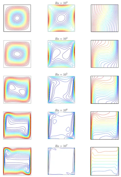
square slot. . . 84 4.12 Natural convection in a square slot, N = 71_×71: Contour plots

for the streamfunction (left), vorticity (middle), and temperature (right) for several Ranumbers. . . 87 4.13 Geometry and boundary conditions for natural convection in a

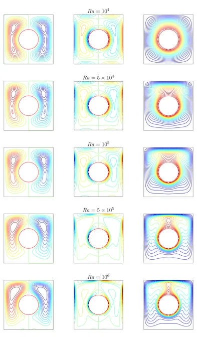
concentric annulus between an outer square cylinder and an inner circular cylinder. . . 88 4.14 Natural convection in a concentric annulus between an outer square

cylinder and an inner circular cylinder, N = 62_×62: Contour plots for the streamfunction (left), vorticity (middle), and temperature (right) for several Ranumbers. . . 89

(19)

List of Figures xvii

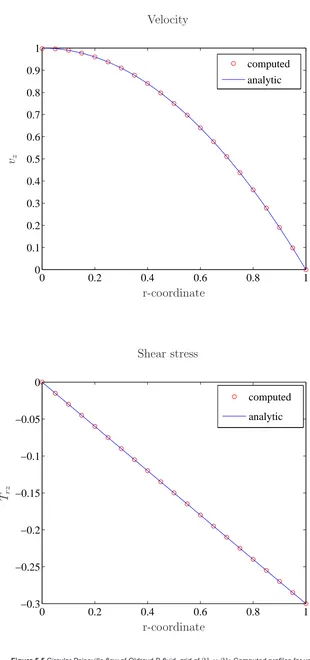
5.2 Geometry for planar Poiseuille flow. The spacing between the two plates is exaggerated in relation to its length. . . 95 5.3 A 2D computational model for planar Poiseuille flow. . . 96 5.4 Boundary conditions for Poiseuille flows. . . 97 5.5 Circular Poiseuille flow of Oldroyd-B fluid, grid of 21_×21:

Com-puted profiles for velocity. . . 103 5.6 Circular Poiseuille flow of Oldroyd-B fluid, grid of 21_×21:

Com-puted profiles for stresses. . . 104 5.7 Geometry of a corrugated tube. . . 105 5.8 Corrugated tube flow of Newtonian fluid, M = 0.16, ǫ = 0.3,

N = 41_×41: Contour plots for the streamfunction and vorticity. . 108 5.9 Corrugated tube flow of Oldroyd-B fluid, W e= 1.2017, N = 31_×

31, M = 0.5, ǫ = 0.1: Contour plots for the field variables. The maximum and minimum values and their locations are also included.110 5.10 Corrugated tube flow of Oldroyd-B fluid, W e = 1.2017, M =

0.5, ǫ= 0.1: Contour plots for the velocity vz (left) and vr (right). The maximum and minimum values of the velocities and their lo-cations are also included. . . 111

6.1 Example 1, Heat equation, N = 101, ∆t = 0.001. Exact and computed solutions at several time levels. . . 118 6.2 Example 1, Heat equation, N = _{11,21,_{· · ·} ,101_}. Error against

grid size at t= 1. The solution converges apparently as O(h4.65_{). . 118} 6.3 Example 1, Heat equation,N = 101, ∆t=_{10−2_,₂_×₁₀−2_,_{· · ·} _,₁₀−1_}_.

Error against time step at t = 1. The solution converges appar-ently as O(∆t1.81_{). . . 119} 6.4 Example 2, N = 201, ∆t = 0.001, x _∈ [₋10π; 10π]. Exact and

numerical solutions at t= 1.5. . . 120 6.5 Example 2, Hyperbolic equation, N = _{11,21,_{· · ·},201_}, ∆t =

0.001, x _∈ [0; 2π]. RMS error against grid size at t = 2. The solution converges asO(h3.53_{) . . . 121} 6.6 Example 3, 1D-Burgers’ Equation. Analytic solution of Burger

equation at various time levels. . . 121 6.7 Example 3, 1D Burger’s equation. Distribution of error over the

spatial domain at t = 0.4 by the DuFort-Frankel explicit (D/F), FTCS explicit, modified Runge-Kutta (MRK), second order TVD scheme (TVD), and present (CL-IRBF) methods. . . 122 6.8 Example 3, 1D Burger’s equation. Distribution of error over the

spatial domain at t = 1 by the DuFort-Frankel explicit (D/F), FTCS explicit, modified Runge-Kutta (MRK), second order TVD scheme (TVD), and present (CL-IRBF) methods. . . 124 6.9 Example 3, 1D Burger’s equation. Variations of the RMS error of

the solution as time step and grid size are reduced. . . 124 6.10 Example 4, Problem 1,t= 0.05. Spatial and temporal convergence

(20)

List of Figures xviii

6.12 Example 5, Grid used for calculating the start-up planar Poiseuille flow. Notice that the boundary conditions for stresses are used for the flow of Oldroyd-B fluid. . . 131 6.13 Example 5, Problem 1, planar Poiseuille flow of Newtonian fluid,

grid spacing h= 0.05. Evolution of velocity at nodes indicated in Figure 6.12. . . 132 6.14 Example 5, Problem 1, planar Poiseuille flow of Newtonian fluid,

h= 0.05. Velocity profiles at different non-dimensional times. No-tice that the velocity profiles att= 1 andt = 5 are indistinguishable.132 6.15 Example 5, Problem 1, planar Poiseuille flow of Newtonian fluid,

t= 0.5: convergence rates of the present method in time and space. 133 6.16 Example 5, Problem 2, planar Poiseuille flow of Oldroyd-B fluid,

W e = 0.5: Evolution of the streamfunction at an interior sample node. . . 136 6.17 Example 5, Problem 2, planar Poiseuille flow of Oldroyd-B fluid,

W e= 0.5: Evolution of the velocity at the centreline node and an interior sample node. . . 136 6.18 Example 5, Problem 2, planar Poiseuille flow of Oldroyd-B fluid,

W e = 0.5. Evolution of shear stress at the wall and an interior sample node. . . 137 6.19 Example 5, Problem 2, planar Poiseuille flow of Oldroyd-B fluid,

W e = 0.5, E = 0.5, h = 0.05. Velocity profiles at different time levels. . . 138 6.20 Example 5, Problem 2, planar Poiseuille flow of Oldroyd-B fluid,

Re= 1: Evolution of the centreline velocity over time with differ-ent values of the elasticity E. . . 138 6.21 Example 5, Problem 2, planar Poiseuille flow of Oldroyd-B fluid,

Re = 1: Evolution of the shear stress at the wall over time with different values of the elasticity E. . . 139 6.22 Example 5, Problem 2, planar Poiseuille flow of Oldroyd-B fluid,

(21)

Chapter 1

Introduction

This chapter aims to give an introduction to the present thesis. It starts with the motivation of the proposed research. Then, brief overviews of the basic equations governing the motion of Newtonian and non-Newtonian fluids, and numerical schemes used for the simulation of fluid flows are given. Next, we review inte-grated radial basis functions (IRBF), which are used to construct the proposed compact stencils, and present the main objectives of the research. The chapter will end with an outline of the thesis.

1.1

Motivation

Computational Fluid Dynamics (CFD) deals with the computer simulation of fluid flows, where the motion of a fluid is described mathematically, e.g., in the form of ODEs and PDEs. A physical/engineering process can be investigated theoretically, experimentally and by computer simulations. Doing experiments and measurements is a traditional approach, and it has been widely used with varying degrees of success. However, this approach suffers from time consuming, high cost, large measurement error, etc. and has limitations - for examples, the size of problems should be small and the obtained information is rather limited. These drawbacks are eliminated in computer simulations (e.g. the problem can now be of small or large size, etc.). Since the late 1960s, the development and application of CFD to all aspects of fluid dynamics have been growing massively (Moin and Kim, 1997). The quality of simulation results depends on the accuracy of the numerical method used. There are numerous numerical methods developed, which can be classified into low order and high order methods, or finite-element-based and meshless/grid-finite-element-based methods. Each group has its own strengths and weaknesses. High-order methods have the ability to produce accurate results using relatively coarse discretisations, while low-order methods result in sparse system matrices that can be solved efficiently. Meshless/grid-based methods are much more efficient in modelling complex geometries than finite-element-based methods.

(22)

1.2. Governing equations 2

capability (Park and Sandberg, 1991). Originally, RBFNs were used for function approximation and classification. Then, RBFNs were extended to a variety of ap-plications, e.g. the solution of ordinary differential equations/ partial differential equations (ODEs/PDEs) (Kansa and Hon, 2000). They have been used with suc-cess in solving heat transfer problems (Zerroukat et al., 1998), fluid flow problems (Sadat and Couturier, 2000; Kosec and Sarler, 2011), time-dependent problems (Kansa et al., 2004), fluid-structure interaction analyses (Ngo-Cong et al., 2012b), Darcy flows (Kosec and Sarler, 2008), hyperbolic problems (Islam et al., 2013), etc. - this list is not meant to be exhaustive. RBFNs are a flexible simulation method as they can be used with Cartesian grids or meshless discretisations, and employed in local or global forms derived from the differentiation or integration process. We will develop approximation stencils based on RBFNs for fluid flows, where the benefits of low cost (by means of Cartesian grids), sparse system matri-ces (using small stencils) and high order accuracy (integrated RBFs and compact form) of the existing numerical schemes are exploited.

1.2

Governing equations

1.2.1 Newtonian and non-Newtonian fluids

Fluids are substances whose deformation easily occurs under external shear forces. Indeed, applying a very small force is able to result in the fluid motion. Fluids can be recognised everywhere in human life, e.g. breathing, blood, wind, rain, etc., and also in many industrial disciplines, such as aerospace, automotive, food processing and chemical processing. An understanding of the behaviour of fluids allows us to control effectively their effects in flow processes.

Fluids can be divided into Newtonian and non-Newtonian. If the behaviour of a fluid is linear, one has a Newtonian fluid; otherwise, a non-Newtonian fluid. Viscoelastic is the term used to describe the coexistence of elastic and viscous properties in a fluid. Viscoelastic fluid is an example of non-Newtonian fluids. Because of the mixture, viscoelastic fluids exhibit many interesting phenomena, which are totally different from those associated with Newtonian fluids.

There are different fluid flow regimes, ranging from creeping, through laminar to turbulent. The laminar regime is characterised by the smooth motion of a fluid, while the turbulent regime tends to produce chaotic eddies, vortices and other flow instabilities. At speeds that are low enough, the creeping flow is observed. As the speed is increased, the flow is then said to be laminar. Further increases in speed may cause the instability in the fluid, which corresponds to a turbulent regime. A dimensionless quantity, called the Reynolds number Re, can be used to characterise these regimes. Creeping flow is the flow at Re= 0, laminar flow occurs at low Reynolds numbers, and turbulent flow occurs at high Reynolds numbers. When dealing with the flow at high Reynolds numbers, the non-linear term in the governing equation will be dominant, which makes the numerical solution difficult to converge, and special care is needed.

(23)

more challenging than that of Newtonian fluid flows (Keunings, 1990; Walters and Webster, 2003). Constitutive equations relating stress to rate of strain are nonlinear for non-Newtonian fluids, and consequently, their solutions are obtained normally in a more complex manner than those associated with the Newtonian case (Walters and Webster, 2003; Barnes et al., 1989; Macosko, 1994; Grillet et al., 1999). For viscoelatic fluids, a dimensionless quantity, called the Weissenberg numberW e, is used to measure the relative importance of the elastic and viscous effects.

1.2.2 Conservation laws

The motion of any fluid is described by the equations of conservation of mass, mo-mentum and energy. Consider an incompressible fluid, whose density is constant. The conservation of mass can be described as

∇ ·v= 0, x_∈Ω, (1.1)

wherevis the velocity vector,xthe position vector, and Ω the domain of interest. The conservation of momentum (equation of motion) is given by

ρDv

Dt = (∇ ·σ) +ρg, x∈Ω, (1.2)

where t is the time, ρ the density, σ _{the total stress tensor,} _g _{the force per unit}

mass due to gravity, and D/Dt the material or substantial derivative (Tanner, 2000; Reddy and Gartling, 1994),

D Dt =

∂

∂t +v· ∇ (1.3)

The total stress tensor σ _{for a fluid at rest is} σ ₌ ₋_p_{I, in which} _p _{is called the}

hydrostatic pressure, and I is the identity tensor. When dealing with fluids in motion, the total stress tensor is decomposed into two parts: σ ₌₋_p_I₊τ_{, where} τ _{is the extra stress tensor. Equation (1.2) can thus be rewritten as}

ρDv

Dt =−∇p+ (∇ ·τ) +ρg, x∈Ω. (1.4)

For simplicity, without loss of generality, one may combine the pressure and gravity terms into the so-called “modified pressure”: _∇P =_∇p₋ρg.

1.2.3 Constitutive equations

The constitutive equation describes the relation between force and deformation in fluid. Constitutive equations are usually written in terms of extra stress tensor

τ _{and strain rate tensor. The simplest constitutive equation is in the case of}

Newtonian fluids

(24)

where η0 is the constant viscosity, and 2D is the rate of deformation tensor, defined as 2D = _∇vT +_∇v.

Many differential constitutive models have been developed. Below is a brief review of some constitutive models.

Upper-Convected Maxwell (UCM) model

τ ₊_λ₁τ∇_{= 2}_η₀_D_, _(1.6)

whereλ1 is the characteristic relaxation time of the fluid and the upper-convected derivative

∇

[] is defined as

∇ [] = ∂[]

∂t +v· ∇[]−(∇v)

T

·[]₋[]_{· ∇}v. (1.7)

Oldroyd-B model

τ ₊_λ₁τ∇_{= 2}_η₀

D+λ2 ∇ D

, (1.8)

where λ2 is the characteristic retardation time of the fluid. Let α be the ratio of the retardation time to the relaxation time (α = λ2/λ1). The Oldroyd-B model will reduce to UCM when α= 0.

The extra stress tensor τ _{can also be decomposed into two components, namely}

solvent and polymeric contributions

τ _{= 2}_η_sD+τ_v_, _(1.9)

where ηs is the solvent viscosity and τv is the elastic stress

τ_v₊_λ₁τ∇_v _{= 2}_η_p_D_, _(1.10)

in which ηp is the polymeric viscosity. Note that η0 = ηs+ηp, ηs = αη0, and

ηp = (1−α)η0. If the value of ηs in equation (1.9) is set to zero (i.e. τ = τv), the Oldroyd-B model reduces to a UCM model. Further details can be found in (Covas et al., 1995) and (Phan-Thien and Tanner, 1977).

Giesekus-Leonov model

τ_v₊_λ₁τ∇_v₋ λ1

2ηp{

τ_v_·τ_v_}_{= 2}_η_pD. (1.11)

Phan-Thien Tanner (PTT) model 1

exp

λ1ε

ηp

tr(τ_v₎

τ_v ₊_λ₁τ∇_v₊_ξλ₁_{_D_·τ_v ₊τ_v _·_D_}_{= 2}_η_p_D_, _(1.12)

where ε and ξ are the material parameters, and ‘tr’ denotes the trace operation.

Phan-Thien Tanner (PTT) model 2

1 + λ1ε

ηp

tr(τ_v)

(25)

In this project, we restrict our attention to Newtonian fluids and Oldroyd-B fluids in two dimensional flows. There are three popular forms of the governing equations, based either on velocity-pressure, or streamfunction-vorticity (ψ₋ω) or streamfunction (ψ). Advantages of the (ψ₋ω) formulation over the (v₋p) one are that (i) the number of equations to be solved are reduced due to the elimination of the pressure variable, and thus reducing the computational effort; and (ii) the continuity equation is automatically satisfied. However, one needs to derive a boundary condition for ω from the given boundary conditions, and also to compute the velocities and pressure after solving the system of discrete equations. Advantages of the (ψ) formulation over the (ψ₋ω) one are that (i) the number of equations are further reduced; and (ii) there is no intermediate variable. However, one needs to deal with the approximation of high-order derivatives and the imposition of double boundary conditions. Further details can be found in (Quartapelle, 1993). Some detailed forms of the governing equations are given below, with our focus on the streamfunction-vorticity formulation which is mainly used in the following chapters.

Newtonian fluids:

In Cartesian coordinates, the governing equations for Newtonian fluids take the form

∂vx

∂x + ∂vy

∂y = 0, (1.14)

ρ

∂vx

∂t +vx ∂vx

∂x +vy ∂vx

∂y

=₋∂P

∂x +η0

∂2_v x

∂x2 +

∂2_v x ∂y2 , (1.15) ρ ∂vy

∂t +vx ∂vy

∂x +vy ∂vy

∂y

=₋∂P

∂y +η0

∂2_v y

∂x2 +

∂2_v y

∂y2

. (1.16)

By introducing

x∗ = x

L, y

∗ ₌ y

L, t

∗ ₌ t

L/V ,

p∗ = P

ρV2, v ∗ x =

vx

V , v

∗ y =

vy

V ,

where L and V are the flow characteristic length and velocity, respectively, the governing equations in dimensionless form are obtained

∂v∗ x

∂x∗ +

∂v∗ y

∂y∗ = 0, (1.17)

∂v∗ x

∂t∗ +v ∗ x

∂v∗ x

∂x∗ +v ∗ y

∂v∗ x

∂y∗ =−

∂p∗

∂x∗ + 1

Re

∂2_v∗ x

∂x∗2 +

∂2_v∗ x

∂y∗2

, (1.18)

∂v∗ y

∂t∗ +v ∗ x

∂v∗ y

∂x∗ +v ∗ y

∂v∗ y

∂y∗ =−

∂p∗

∂y∗ + 1

Re

_∂2_v∗ y

∂x∗2 +

∂2_v∗ y

∂y∗2

, (1.19)

in which Re=ρV L/η0 is the Reynolds number.

(26)

for-1.2. Governing equations 6

mulation

∂2_ψ

∂x2 +

∂2_ψ

∂y2 =−ω, (1.20)

∂ω ∂t + ∂ψ ∂y ∂ω ∂x − ∂ψ ∂x ∂ω ∂y = 1 Re

∂2_ω

∂x2 +

∂2_ω

∂y2

, (1.21)

where the streamfunction ψ(x, y, t) is defined with the property: vx =

∂ψ ∂y and

vy =−

∂ψ

∂x, and ω is the vorticity, ω= ∂vy

∂x − ∂vx

∂y .

In cylindrical coordinates (axi-symmetric), the governing equations for Newtonian fluids are of the form

1

r ∂

∂r(rvr) + ∂vz

∂z = 0, (1.22)

ρ

∂vr

∂t +vr ∂vr

∂r +vz ∂vr

∂z

=₋∂p

∂r +η0

∂ ∂r 1 r ∂ ∂r (rvr)

+ ∂ 2_v r ∂z2 , (1.23) ρ ∂vz

∂t +vr ∂vz

∂r +vz ∂vz

∂z

=₋∂p

∂z +η0

1 r ∂ ∂r

r∂vz ∂r +∂ 2_v z ∂z2 . (1.24)

Their dimensionless form is 1

r∗

∂ ∂r∗ (r

∗_v∗ r) +

∂v∗ z

∂z∗ = 0, (1.25)

πRe

2

∂v∗ r

∂t∗ +v ∗ r

∂v∗ r

∂r∗ +v ∗ z ∂v∗ r ∂z∗

=₋∂p ∗

∂r∗ +

∂ ∂r∗ 1 r∗ ∂ ∂r∗ (r

∗_v∗ r)

+ ∂

2_v∗ r

∂z∗2 , (1.26) πRe 2 ∂v∗ r

∂t∗ +v ∗ r

∂v∗ z

∂r∗ +v ∗ z ∂v∗ z ∂z∗

=₋∂p ∗

∂z∗ +

1 r∗ ∂ ∂r∗

r∗∂v

∗ z

∂r∗

+∂

2_v∗ z

∂z∗2

. (1.27)

where

r∗ = r

R, z

∗ ₌ z

R, t

∗ ₌ t

Q/R3,

p∗ = P

η0Q/R3

, v_r∗ = vr

Q/R2, v ∗ z =

vz

Q/R2,

and Re= 2ρQ

πRη0

is the Reynolds number.

The streamfunction-vorticity formulation in cylindrical coordinates becomes

1

r

∂2_ψ

∂r2 +

∂2_ψ

∂z2 − 1

r ∂ψ

∂r

=₋ω, (1.28)

πRe

2

∂ω ∂t +vz

∂ω ∂z +vr

∂ω ∂r − vr r ω = ∂ 2_ω

∂r2 + 1

r ∂ω

∂r − ω r2 +

∂2_ω

∂z2, (1.29)

where vr =− 1

r ∂ψ

∂z and vz =

1

r ∂ψ

∂r, and ω= ∂vr

∂z − ∂vz

∂r .

(27)

Oldroyd-B fluids:

In Cartesian coordinates, the dimensionless form of the governing equations for Oldroyd-B fluids is

∂2_ψ

∂x2 +

∂2_ψ

∂y2 +ω = 0, (1.30)

Re

∂ω ∂t +vx

∂ω ∂x +vy

∂ω ∂y

=

∂2_τ xy

∂x2 −

∂2_τ xy

∂y2 −

∂2₍_τ

xx−τyy)

∂x∂y

+α

∂2_ω

∂x2 +

∂2_ω

∂y2

, (1.31)

τxx+W e

∂τxx

∂t +vx ∂τxx

∂x +vy ∂τxx

∂y −2 ∂vx

∂xτxx−2 ∂vx

∂y τxy

= 2(1₋α)∂vx

∂x, (1.32)

τxy +W e

∂τxy

∂t +vx ∂τxy

∂x +vy ∂τxy

∂y −

∂vx

∂y τyy− ∂vy

∂xτxx

= (1₋α) ∂vx ∂y + ∂vy ∂x , (1.33)

τyy+W e

∂τyy

∂t +vx ∂τyy

∂x +vy ∂τyy

∂y −2 ∂vy

∂xτxy−2 ∂vy

∂y τyy

= 2(1₋α)∂vy

∂y , (1.34)

whereRe= ρV L

η0

is the Reynolds number,W e=λ1

V

L is the Weissenberg number,

and L and V are the flow characteristic length and velocity, respectively.

(28)

1.3. Conventional simulation methods 8

Oldroyd-B fluids, flowing in a tube with circular cross sections, is

1

r

∂2_ψ

∂r2 +

∂2_ψ

∂z2 − 1

r ∂ψ

∂r

+ω = 0, (1.35)

πRe

2

∂ω ∂t +vz

∂ω ∂z +vr

∂ω ∂r − vr rω =α

∂2_ω

∂r2 + 1

r ∂ω ∂r −

ω r2 +

∂2_ω

∂z2 +∂ 2_τ rr ∂r∂z − ∂2_τ

rz

∂r2 +

∂2_τ rz

∂z2 + 1 r ∂τrr ∂z − ∂τθθ ∂z − ∂ 2_τ zz ∂r∂z + 1

r2τrz− 1

r ∂τrz

∂r , (1.36)

τrr+W e

∂τrr

∂t +vr ∂τrr

∂r +vz ∂τrr

∂z −2 ∂vr

∂r τrr−2 ∂vr

∂z τrz

= 2(1₋α)∂vr

∂r , (1.37)

τrz+W e

∂τrz

∂t +vr ∂τrz

∂r +vz ∂τrz

∂z +

vr

r τrz − ∂vz

∂r τrr− ∂vr

∂z τzz

= (1₋α) ∂vr ∂z + ∂vz ∂r , (1.38)

τzz+W e

∂τzz

∂t +vr ∂τzz

∂r +vz ∂τzz

∂z −2 ∂vz

∂r τrz −2 ∂vz

∂z τzz

= 2(1₋α)∂vz

∂z , (1.39)

τθθ+W e

∂τθθ

∂t +vr ∂τθθ

∂r +vz ∂τθθ

∂z −2 vr

r τθθ

= 2(1₋α)vr

r , (1.40)

whereRe= 2ρQ

πRη0

andW e=λ1

Q

R3 are the Reynolds number and the Weissenberg number, respectively, R is the radius of the tube andQ is the flow rate.

1.3

Conventional simulation methods

(29)

1.3. Conventional simulation methods 9

few FDM publications in Computational Rheology, where only flows with simple geometries are considered. On the other hand, FEMs, BEMs and FVMs can accurately handle problems with complex geometries. For these techniques, gen-erating a mesh and re-meshing are known to be a time-consuming process (Pastor et al., 1991) and the solution appears to converge very slowly in high gradient regions (Emdadi et al., 2008). FEMs have been used in solving transient prob-lems (Bishko et al., 1999; Wapperom et al., 2000), and non-Newtonian fluid flows (Rasmussen, 1999; Yurun and Crochet, 1995; Fan et al., 1999; Sun et al., 1999). In FVMs, physical quantities such as mass, momentum and energy are exactly conserved over any control volume, and thus over the whole domain of interest. Therefore, even with a coarse grid, FVMs can give a solution that exhibits the ex-act integral balance (Eymard et al., 2000). BEMs can be used to solve linear and nonlinear problems, where one can avoid taking the variables at interior nodes as the unknowns in the discretisation system. This feature comes straightforwardly for solving linear problems, but for non-linear problems, to make it occur, some extra treatments need be implemented. BEMs generate a full matrix and do not work well for highly nonlinear flows (Tanner and Xue, 2002).

Based on their order of convergence, numerical methods can be classified into low order and high order. Low-order methods are referred to as methods of first and second orders of convergence, e.g. traditional FDMs, FEMs, FVMs, and BEMs. Their approximations are widely based on linear functions. The main advantages of these methods are their simplicity, which results in fast implemen-tation, and robustness (the robustness means that one can always get a solution, even though it may not be very accurate). However, one needs to use a large number of grid points to represent the approximate solution and thus requiring large computational resources. Most of problems in practice are large scale; low rates of convergence may hinder low-order methods from being useful.

(30)

1.4. Integrated radial basis function methods 10

been presented for the flow of viscoelastic fluids through an undulating tube in the transformed coordinates system, and highly accurate results are obtained. There are several ways proposed in the literature to handle irregularly shaped domains, including domain decompositions, coordinate transformations, fictitious domains and meshless approximations (Bueno-Orovio et al., 2006). It is noted that the access of nodes in meshless approximations and Cartesian-grid-based approximations are much faster than the node access in approximations based on unstructured meshes (Liu et al., 2006).

Numerical methods can also be classified into global and local. For the former, the value of a derivative at a point is computed from the values of the field variable at all nodes in the domain. Such approximations can result in better accuracy, as shown in spectral methods, DQMs and RBFNs. However, global methods are geometrically less flexible and more complicated to implement. They provide dense matrices whose condition numbers grow rapidly as the number of nodes are increased. Handling the fully populated matrices becomes very costly in the case of large scale problems. For local methods, such as FDMs, FEMs and FVMs, the approximation of a derivative at a point involves the neighbouring nodal points only. They can provide resultant sparse coefficient matrices, and thus, their solution are more efficient. Local methods, on the other hand, converge slowly with grid/mesh refinement and cannot yield highly accurate results. Many efforts have been put in the improvement of accuracy for local methods. Using local approximations compactly is an attractive prospect.

1.4

Integrated radial basis function methods

Radial basis function networks are a powerful concept, which is essential to this project. Derived from the biological sciences, they can be considered as univer-sal approximation schemes (Haykin, 1999). The application of RBFNs for the numerical solution of partial differential equations (PDEs) was first reported by Kansa (1990) (Kansa, 1990). A function f(x) can be represented by RBFs as

f(x) = N X

i=1

wigi(x), (1.41)

where x is the position vector, N is the number of RBFs, _{wi}N_i=1 is the set of network weights, and _{gi(x)}Ni=1 is the set of RBFs. The RBFs can be written in a general form as gi(x) =gi(kx−cik), where k · k denotes the Euclidean norm and _{ci}Ni=1 is a set of the RBF centers. There are some common types of RBFs, including

• Multiquadrics function (MQ)

gi(x) = q

r2₊_a2

i, ai >0, (1.42)

• Inverse multiquadrics function

gi(x) = p 1

r2₊_a2 i

(31)

1.4. Integrated radial basis function methods 11

• Gaussians function

gi(x) = exp

−r

2

a2 i

, ai >0, (1.44)

where ai is usually referred to as the width of the ith basis function and r =

kx₋c_i_k=p(x₋c_i)_·(x₋c_i).

Some RBFs, such as the above mentioned, are shown to possess spectral conver-gence rate. Thus, they fall into a class of high order methods. RBF collocation methods need only a set of discrete points – instead of a set of elements – through-out a volume to approximate the field variables. Thus, they can be regarded as truly meshless methods. Originally, RBF approximations were constructed glob-ally. Advantages of global RBF schemes include (i) fast convergence (spectral accuracy for some RBFs such as the multiquadric and Gaussian functions); (ii) meshless nature and (iii) simple implementation. Unlike other high order meth-ods, RBFNs are capable of handling domains with non-rectangular boundaries. To overcome the problem of fully populated matrices and their high condition numbers of global methods, local RBF methods were developed (Franke, 1982; Shu et al., 2003; Kosec and Sarler, 2008; Bourantas et al., 2010). A much larger number of nodes can be now employed; but, their solution accuracy is significantly reduced (Lee et al., 2003). Compact local RBF schemes have been implemented, e.g. (Mai-Duy and Tran-Cong, 2011), to enhance the numerical accuracy of local forms.

RBF approximations can be obtained from the differentiation process (differenti-ated RBFs (DRBFs)) or the integration process (integr(differenti-ated RBFs (IRBFs)). In DRBFs, the function to be approximated is first decomposed into RBFs, and its derivatives are then calculated by differentiating RBFs

u(x) = N X

i=1

wigi(x), (1.45)

∂k_u_(x)

∂ηk = N X

i=1

w_i[η]h(k)_[η]i(x), (1.46)

where η denotes a component of the position vector x (e.g. η can be x for 1D problems, and x or y for 2D problems), superscript (k) denotes the order of the

derivatives of u, andh(k)_[η]i(x) = ∂ k_g_i(x)

∂ηk .

(32)

de-1.5. Objectives of the research 12

pendent variable itself are then obtained by integrating RBFs

∂k_u_(x)

∂ηk = N X

i=1

w_i[η]gi(x) = N X

i=1

w_i[η]I_[η]i(k)(x), (1.47)

∂k−1_u_(x)

∂ηk−1 = N X

i=1

w_i[η]I_[η]i(k−1)(x) +C₁[η], (1.48)

· · ·

u(x) = N X

i=1

w_i[η]I_[η]i(0)(x) + η k−1 (k₋1)!C

[η] 1 +

ηk−2 (k₋2)!C

[η]

2 +· · ·+C [η]

k , (1.49)

where I_[η]i(k−1)(x) = R I_[η]i(k)(x)dη, _{· · ·}, I_[η]i(0)(x) = R I_[η]i(1)(x)dη; and C₁[η], C₂[η],_{· · ·} , C_k[η]

are the “constants” of integration, which will be constants for 1D problems, func-tions in one variable for 2D problems, and in two variables for 3D problems. These functions are unknown and can be approximated as linear combinations of basis functions.

The purposes of using integration (a smoothing operator) to construct the approx-imants are to avoid the reduction in convergence rate caused by differentiation and to improve the numerical stability of a discrete solution. It has been found that the integration constants are very helpful in the implementation of multiple boundary conditions (Mai-Duy, 2005; Mai-Duy and Tanner, 2005b; Mai-Duy and Tran-Cong, 2006) and non-overlapping domain decompositions (Mai-Duy and Tran-Cong, 2008b). Numerical results showed that IRBFs yield better accuracy than DRBFs (Mai-Duy and Tran-Cong, 2001, 2003; Mai-Duy, 2005; Mai-Duy and Tanner, 2005b).

1.5

Objectives of the research

This research project is concerned with the development of powerful approxima-tion stencils for the discretisaapproxima-tion of partial differential equaapproxima-tions (PDEs) gov-erning the motion of fluids. The proposed stencils are based on several recent advances in computational fluid dynamics and computational mechanics, includ-ing the integral approximation formulation, radial basis functions (RBFs) and compact approximations. The main objectives of this research are

• to build up compact local integrated RBF (CLIRBF) stencils for the ap-proximation of a function and its derivatives up to fourth order

• to introduce CLIRBF stencils into the point collocation formulation for the discretisation of second-order elliptic equations and biharmonic equations

• to introduce CLIRBF stencils into the sub-region collocation formulation for the discretisation of second-order elliptic equations

• to build up a numerical procedure based on CLIRBF stencils and point collocation for the simulation of Newtonian fluid flows

(33)

1.6. Outline of the Thesis 13

• to build up a numerical procedure based on CLIRBF stencils and point collocation for the simulation of viscoelastic fluid flows

1.6

Outline of the Thesis

The remaining of the thesis is organised as follows.

• Chapter 2 deals with the development of several CLIRBF stencils for solving fourth-order ODEs and PDEs in point collocation. Test problems, governed by the biharmonic equation and its equivalent set of two Poisson equations, are considered.

• Chapter 3 deals with the incorporation of CLIRBF stencils into the point-collocation formulation for the simulation of flows of a Newtonian fluid. Test problems, whose solutions involve very steep gradients, are considered. Governing equations employed are the convection-diffusion equation and the streamfunction-vorticity formulation.

• Chapter 4 deals with the incorporation of CLIRBF stencils into the subregion-collocation formulation for the simulation of flows of a Newtonian fluid. Two numerical integration schemes to evaluate volume integrals, namely the middle point rule and 3-point Gaussian quadrature rule, are employed. Several test problems including natural convection in an annulus, where the governing equations are taken in the streamfunction-vorticity formulation, are considered.

• Chapter 5 is concerned with the application of CLIRBF stencils for simu-lating steady state viscoelastic flows. Poiseuille flows and corrugated tube flows of Oldroyd-B fluids are considered.

• Chapter 6 is concerned with the use of CLIRBF stencils in transient prob-lems. Hyperbolic and parabolic equations are considered.

(34)

Chapter 2

Compact local IRBF stencils and point

collocation for high-order differential

problems

Our first concern is about high-order ODEs/PDEs, which govern many applica-tions in engineering. New compact local stencils based on IRBFs for the discreti-sation of fourth-order ODEs and PDEs will be presented in this chapter. Five types of compact stencils - 3-node and 5-node for 1D problems and 5_×5-node, 13-node and 3_×3 -node for 2D problems - are implemented. In the case of 3-node stencil and 3_×3-node stencil, nodal values of the first derivative(s) of the field variable are treated as additional unknowns (i.e. 2 unknowns per node for 3-node stencil and 3 unknowns per node for 3_×3-node stencil). The integration constants arising from the construction of IRBFs are exploited to incorporate into the local IRBF approximations (i) values of the governing equation (GE) at selected nodes for the case of 5-, 5_×5- and 13-node stencils, and (ii) not only nodal values of the governing equation but also nodal values of the first derivative(s) for the case of 3-node stencil and 3_×3-node stencil. There are no special treatments required for grid nodes near the boundary for 3-node stencil and 3_×3-node stencil. The proposed stencils, which lead to sparse system matrices, are numerically verified through the solution of several test problems.

2.1

Introduction

(35)

2.2. Brief review of integrated RBFs 15

2009b), and Galerkin schemes (Mai-Duy et al., 2009a). Global RBF methods are more accurate but less efficient than local RBF methods (please see Section 1.4 for a detailed discussion).

This chapter is concerned with the development of local IRBF stencils in com-pact form for the solution of fourth-order ODEs and PDEs. The following two strategies (e.g. (Stephenson, 1984; Altas et al., 1998)) are studied in the context of local compact IRBF stencils.

The first strategy employs relatively large stencils (i.e. 5 nodes for 1D fourth-order problems, and 13 nodes or 5_×5 nodes for 2D fourth-order problems). For this approach, only nodal values of the field variable on a stencil are treated as unknowns. It is noted that, when compared with second-order problems, there are more nodes used on a stencil (i.e. 2 additional nodes for 1D problems, and 4 and 16 additional nodes for 2D problems).

The second strategy employs relatively small stencils (i.e. 3 nodes for 1D problems and 3 _×3 nodes for 2D problems). For this approach, not only nodal values of the field variable on a stencil but also nodal values of its first derivative at selected nodes are treated as unknowns. Advantages of this strategy include (i) the number of nodes employed here does not increase when compared with the case of second-order problems; (ii) there are no special treatments required for grid nodes near the boundary; (iii) boundary derivative values can be imposed easily and accurately; and (iv) first derivative values are obtained directly from the final system of algebraic equations.

Furthermore, in both strategies, we also incorporate nodal values of the governing equation at selected nodes on a stencil into the IRBF approximations. Numerical results will show that such an incorporation can significantly enhance the solution accuracy.

The remainder of the chapter is organised as follows. Section 2 is a brief review of IRBFs. The proposed compact local stencils based on IRBFs are presented for 1D problems in Section 3 and for 2D problems in Section 4. Numerical examples, including the simulation of lid-driven cavity flows, are given in Section 5 to demonstrate the attractiveness of the proposed stencils. Section 6 concludes the chapter.

2.2

Brief review of integrated RBFs

(36)

2.2.1 Second-order integrated RBF scheme

In this scheme, the second-order derivatives of the function u are decomposed into a set of RBFs

∂2_u_(x)

∂η2 = N X

i=1

w_i[η]I_[η]i(2)(x), (2.1)

where η denotes a component of the position vector x (e.g. η can be x for 1D problems, and x or y for 2D problems), _{wi}N_i=1 is the set of RBF coefficients

which are unknown, and nI_i(2)(x)oN

i=1 is the set of RBFs. Expression (2.1) is then integrated to obtain approximate expressions for lower order derivatives and the function itself as follows.

∂u(x)

∂η =

N X

i=1

w[η]_i I_[η]i(1)(x) +C1, (2.2)

u(x) = N X

i=1

w[η]_i I_[η]i(0)(x) +ηC1+C2, (2.3)

where C1 and C2 are “constants of integration” with respect to η, which are to be treated as the additional RBF coefficients. In (2.1)-(2.3), the superscript (.) is used to indicate the associated derivative order.

Collocating (2.1)-(2.3) at a set of nodal points _{xi}N_i=1 yields d

∂2_u

∂η2 =H (2)

η wbη, (2.4)

c

∂u ∂η =H

(1)

η wbη, (2.5)

b

u=_H_η(0)w_bη, (2.6)

where the notation ‘_b’ is used to denote a vector, _H(.) _{is the RBF coefficient} matrix in the RBF space and wbη is the RBF vector of coefficients, including the integration constants.

2.2.2 Fourth-order integrated RBF scheme

In this scheme, the fourth-order derivatives of the functionuare decomposed into a set of RBFs as

∂4u(x)

∂η4 = N X

i=1

w_i[η]I_[η]i(4)(x). (2.7)

(37)

∂3_u_(x)

∂η3 = N X

i=1

w[η]_i I_[η]i(3)(x) +C1, (2.8)

∂2_u_(x)

∂η2 = N X

i=1

w[η]_i I_[η]i(2)(x) +ηC1+C2, (2.9)

∂u(x)

∂η =

N X

i=1

w[η]_i I_[η]i(1)(x) + η 2

2C1+ηC2+C3, (2.10)

u(x) = N X

i=1

w[η]_i I_[η]i(0)(x) + η 3 6C1+

η2

2 C2+ηC3+C4. (2.11)

Collocating (2.7)-(2.11) at a set of nodal points _{xi}N_i=1 yields d

∂4_u

∂η4 =H (4)

η wbη, (2.12)

d

∂3_u

∂η3 =H (3)

η wbη, (2.13)

d

∂2_u

∂η2 =H (2)

η wbη, (2.14)

c

∂u ∂η =H

(1)

η wbη, (2.15)

b

u=_H(0)_η w_bη. (2.16)

For the approximations of integration constants used in (2.1)-(2.3) and (2.7)-(2.11), the reader is referred to (Mai-Duy and Tran-Cong, 2003, 2010) for further details.

In this study, the multiquadric (MQ) function is chosen as the basis function as

I_i(4)(x) = q

(x₋ci)2+a2i for 1D problems, (2.17)

I_i(4)(x) = q

(x₋cix)2_{+ (}_y₋_c_iy)2₊_a2

i for 2D problems, (2.18)

where ci (for 1D problems) or (cix, ciy)T (for 2D problems) and ai are the MQ centre and width, respectively. The width of the ith MQ can be determined according to the following relation

ai =βdi, (2.19)

(38)

2.3. Proposed compact local IRBF stencils for fourth-order ODEs 18

methods. For the latter, one can vary the value of β and/or refine the spatial discretisation to enhance the solution accuracy.

In the following sections, to simplify the notations, we will drop the subscript

η used in (2.12)-(2.16) for 1D problems, and use (i, j) to represent a grid node located at (xi, yj) in a global 2D grid, xk to represent a grid nodek in a local 2D stencil, and _M(i,:) to denote the ith row of the matrix_M.

2.3

Proposed compact local IRBF stencils for fourth-order

ODEs

Our sample of fourth-order ODEs is taken as

d4u dx4 +

d2u

dx2 =f(x), (2.20)

where xA ≤ x ≤xB and f(x) is some given function. The boundary conditions prescribed here are of Dirichlet type, i.e. u and du/dx given at both xA and xB.

We discretise the problem domain using a set of N discrete nodes _{xi}Ni=1, and utilise fourth-order IRBF schemes to represent the field variable u.

2.3.1 Compact local 5-node stencil (5-node CLS)

Consider a grid node xi and its associated 5-node stencil [xi1, xi2, xi3, xi4, xi5] (xi ≡

xi 3).

The conversion system, which represents the relation between the RBF space and the physical space, is established from the following equations

b

u

b

e

=

H(0)

K

| {z }

C

b

w, (2.21)

where _C is the conversion matrix, w_b = (w1, w2, w3, w4, w5, C1, C2, C3, C4)T, ub = (u1, u2, u3, u4, u5)T, bu =H(0)wb are equations representing nodal values of u over the stencil, _H(0) _{is a 5}_×_{9 matrix that is obtained from collocating (2.11) at grid} nodes of the stencil, _be = _Kw_b are equations representing extra information that can be the ODE (2.20) at selected nodes, anddu/dxatxAandxB. Solving (2.21) results in

b

w=_C−1

b

u

b

e

. (2.22)

(39)

derivatives at an arbitrary point x on the stencil are calculated in the physical space as

d4_u₍_x₎

x4 =

h

I₁(4)(x), . . . , I₅(4)(x), 0, 0, 0, 0 iC−1

b u b e , (2.23)

d3_u₍_x₎

dx3 = h

I₁(3)(x), . . . , I₅(3)(x), 1, 0, 0, 0 i

C−1

b u b e , (2.24)

d2_u₍_x₎

dx2 = h

I₁(2)(x), . . . , I₅(2)(x), x, 1, 0, 0 iC−1

b u b e , (2.25)

du(x)

dx =

h

I₁(1)(x), . . . , I₅(1)(x), x2_/₂_{, x,} ₁_, ₀ i_C−1 b u b e , (2.26)

u(x) =h I₁(0)(x), . . . , I₅(0)(x), x3_/₆_{, x}2_/₂_{, x,} ₁ i_C−1 b u b e , (2.27)

where xi

1 ≤ x≤ xi5. In what follows, we present two ways to construct the final system of algebraic equations, namely Implementation 1 and Implementation 2.

Implementation 1: The final system is generated by

(i) the collocation of the ODE (2.20) at_{x3, x4, . . . , xN−2}using (2.23) and (2.25) with x=xi, in whicheb=_Kwb is employed to represent values of (2.20) atxi

2 and

xi

4, i.e.

f(xi 2)

f(xi 4)

=

G(2,:)

G(4,:)

b

w, (2.28)

where _G =_H(4) ₊_H(2)_{, and}

(ii) the imposition of du/dx atxA and xB using (2.26) with x=x1 and x=xN. Implementation 2: The final system is generated by collocating the ODE (2.20) at _{x4, x5, . . . , xN−3} and {x2, x3, xN−2, xN−1}. For the former, the collocation process is similar to that of Implementation 1. For the latter, special treatments for the imposition of first derivative boundary conditions are required. Colloca-tions of the ODE (2.20) at _{x2, x3} and {xN−2, xN−1} are based on the stencils of nodesx3 andxN−2, respectively, with the following modified extra information vectors

b

e= (du(xi

1)/dx, f(xi4))T for the stencil of x3, b

e= (f(xi

2), du(xi5)/dx)T for the stencil of xN−2.

Both implementations lead to a system matrix of dimensions (N ₋2)_×(N ₋2). We define the sparsity as the percentage of zero entries relative to the total matrix entries. For example, the use of grid node N = 31 leads to a system matrix of dimension 29_×29 with the sparsity of 83.82%.

2.3.2 Compact local 3-node stencil (3-node CLS)

Consider a grid node xi (i={2,3, . . . , N −1}) with its associated 3-node stencil [xi

(40)

Unlike the 5-node CLS, nodal values of the first derivative of the field variable are also treated here as unknowns. There are thus two unknowns, namely u and

du/dx, per node.

We form the conversion system as