Stochastic Geometry Analysis and Additional Small Cell Deployment for HetNets Affected by Hot Spots

Research Article

Stochastic Geometry Analysis and Additional Small Cell

Deployment for HetNets Affected by Hot Spots

Nan E and Xiaoli Chu

Department of Electronic and Electrical Engineering, University of Sheffield, Sheffield S1 3JD, UK

Correspondence should be addressed to Xiaoli Chu; [email protected]

Received 7 September 2015; Revised 3 January 2016; Accepted 13 January 2016

Academic Editor: Pedro M. Ruiz

Copyright © 2016 N. E and X. Chu. This is an open access article distributed under the Creative Commons Attribution License, which permits unrestricted use, distribution, and reproduction in any medium, provided the original work is properly cited.

Hot spots (HSs) of mobile users that were not expected in the original network planning may occur after a heterogeneous network (HetNet) has been deployed and affect the network performance. In this case, deploying additional small cells on top of the existing HetNet without changing the existing network infrastructure is considered as a solution. In this paper, we first provide a stochastic geometry analysis for a HetNet affected by a large HS and for the additional small cells that need to be deployed based on the spatial bivariate Poisson point process. The optimal numbers of additional small cells required in the HS and non-HS areas are obtained by minimizing the difference between the numbers of macrocell users after and before the HS occurs based on the analytical results. We then propose an algorithm to maximize the average user throughput by jointly optimizing the locations of additional small cells and user associations of all cells. Simulation results show that the proposed algorithm can maintain the average user throughput above a threshold with excellent fairness among all users even for a very high density of HS users.

1. Introduction

Small cell deployment in heterogeneous networks (HetNets) has been considered as an efficient solution to the rapid growth of mobile data demand under limited radio resources. It is anticipated that deploying low-power small cells will increase the area spectral efficiency [1]. In a HetNet, some small cells are deployed by the users, with their locations uncontrollable by the operators. Moreover, once a HetNet has been deployed, persistent hot spots (HSs) of user equipment (UE) that were not expected in the original network planning may occur, causing extra traffic demand. As the mobile traffic demand goes beyond the network capacity, the quality of service (QoS) of UE in the HetNet will be affected. In this case, deploying additional small cells on top of the existing HetNet by the operators would become necessary.

Considering cost effectiveness for network operators, it is desirable to optimize the number and locations of additional small cells to be deployed without changing the existing HetNet infrastructure. This relies on a thorough analysis of the HetNet. Stochastic geometry and the theory of random geometric graphs have been used in the analysis and design of wireless networks [2]. The internodal distances were modeled

using a spatial bivariate Poisson point process (PPP) in [3]. However, the existence of significant HSs in HetNets has not been specifically considered in stochastic geometry based analysis of mobile networks.

In this paper, we analyse a HetNet before and after an unexpected HS occurs and additional small cells that would be required to mitigate the HS effect under a spatial bivariate PPP model. We model the spatial distributions of different network nodes (e.g., existing small cells, additional small cells to be deployed, HS UE, and non-HS UE) into five possible events. By minimizing the difference between the amounts of macrocell UE after and before the HS occurs based on the analytical results, the optimal numbers of additional small cells required for the HS and non-HS areas are obtained. We then propose an algorithm to maximize the average UE throughput in a HetNet affected by unexpected HS by jointly optimizing the locations of additional small cells on top of the existing HetNet and the user associations of all cells. The relationship between HS UE intensity and additional small cell intensities in HS and non-HS areas is analysed. The sim-ulation results show that our proposed algorithm can effec-tively maintain the average UE throughput requirement with Volume 2016, Article ID 9727891, 9 pages

excellent fairness among all UE even for a very high intensity of HS UE.

The rest of the paper is organized as follows. In Section 2, the system model is presented. The analysis based on the spatial bivariate PPP and the analytical results are provided in Section 3. The optimization of additional small cell deploy-ment and the algorithm to solve it are provided in Section 4. Simulation results and performance evaluation are presented in Section 5. Conclusions are drawn in Section 6.

2. Related Work

Using the stochastic geometry analysis, the authors of [3] studied the distribution of the distances between an arbitrary point and its dissimilar neighboring points as a spatial bivariate Poisson point process. In this paper we will extend the model of [3] into five events for our stochastic geometry analysis in Section 3.

As for small cell deployment in HetNets, the femtocell deployment with an arbitrary topology was optimized by maximizing the number of users supported with QoS con-straints in [4]. In [5], the deployment locations of macro base stations (BSs), pico-BSs, and relays are optimized by selecting a subset of candidate sites. In [6], the locations of small cells are sequentially determined by maximizing the weighted sum of the received signal strength and load, but without consider-ing the user associations. The small cell deployment strategy in [7] considering the movement of UE is proposed.

Although HS mitigation has been studied for wireless sensor networks [8], most existing works on small cell deploy-ment strategies have focused on optimizing the deploydeploy-ment of small cells on top of a conventional macrocell network or the deployment of a whole new HetNet from scratch [4–6]. In [9], the dynamic placement of small cells for hot spots is optimized by minimizing the data delivery cost and by mini-mizing macrocell utilization, respectively, where the locations of additional small cells are chosen from the set of known can-didate sites. As a result, the maximum number of additional small cells is limited by the number of candidate locations.

3. System Model

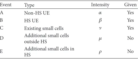
We consider a two-tier HetNet that contains macrocells and small cells. In each macrocell coverage area, the location of the macro-BS is constant, while the small cell BSs and UE are considered as random points [10]. Based on the spatial bivariate PPP [3], we define five events for the problem of deploying additional small cells on top of an existing HetNet as presented in Table 1. Event A represents non-HS UE (which is not jointly distributed with event C, which will be explained later), with the spatial intensity𝛼. Event B denotes the HS UE (which is not jointly distributed with event E, which will be explained later) in the HS area with the spacial intensity𝛽. Since the HS area overlaps with the macrocell coverage, non-HS UE may also occur in the non-HS area. Event C represents the existing small cells. We assume that each existing small cell serves at least one non-HS UE and that each existing small cell BS is jointly distributed with a non-HS UE. Hence, event C is considered as an existing small cell and a non-HS

Table 1: Events.

Event Type Intensity Given

A Non-HS UE 𝛼 Yes

B HS UE 𝛽 Yes

C Existing small cells ] Yes

D Additional small cells

outside HS 𝜇 No

E Additional small cells in

HS 𝜌 No

UE jointly occurring at a random point𝑦. Event D denotes additional small cells that will be deployed in non-HS areas, with intensity 𝜇. Event E denotes additional small cells deployed in the HS area with intensity𝜌, each serving at least one HS UE. Thus, each event E node is jointly distributed with a HS UE.

After a significant HS occurs and additional small cells are deployed, the overall spatial intensity of small cells in non-HS areas is]+ 𝜇and that of small cells in the HS area is]+ 𝜌[11]. For event C, denote 𝑓₁(‖𝑥_U − 𝑦‖) and 𝑔₁(‖𝑥_S − 𝑦‖) as the probability density functions (PDFs) of a UE at𝑥_U and an existing small cell at𝑥_S when event C occurs at𝑦, respectively. Zero-mean isotopic Gaussian distributions with standard deviations 𝜎_𝑓1 and 𝜎_𝑔1 are chosen for 𝑓₁(𝑋) and

𝑔₁(𝑋), respectively [3].

Before the HS occurs, the probability of event C occurring at any point in the macrocell coverage area is calculated as [3]

Pr{C} = ℎ₁(𝑥_U, 𝑥_S)

≜ ∫

𝑦∈RM

𝑓_{1(󵄩󵄩󵄩󵄩𝑥U− 𝑦󵄩󵄩󵄩󵄩) 𝑔1(󵄩󵄩󵄩󵄩𝑥S− 𝑦󵄩󵄩󵄩󵄩) 𝑑𝑦}

= ℎ₁(𝑥_U− 𝑥_S, 0) = ℎ₁(𝑋₁, 0)

= 1 2𝜋𝜎2

1

𝑒−‖𝑋1‖2/2𝜎21,

(1)

whereR_Mis the macrocell coverage area,𝑋₁= 𝑥_U− 𝑥_S, and

𝜎2₁= 𝜎_𝑓2₁+𝜎_𝑔2₁, which is a correlation factor that is determined by the distance of a non-HS UE to its jointly distributed existing small cell BS for event C.

Similarly, for event D, denote𝑓₂(‖𝑥_HSU−𝑦‖)and𝑔₂(‖𝑥_NS−

𝑦‖)as the PDFs for a HS UE occurring at𝑥_HSUand an addi-tional small cell BS deployed at𝑥_NSin the HS area, respec-tively.𝑓₂(𝑋)and𝑔₂(𝑋)are zero-mean isotopic Gaussian dis-tributions with standard deviations𝜎_𝑓2and𝜎_𝑔2, respectively. The probability of a joint event between a HS UE at𝑥_HSUand an additional small cell BS at𝑥_NSoccurring in the HS area is given by [3]

ℎ2(𝑥HSU, 𝑥NS)

≜ ∫

𝑦∈RH

𝑓_{2(󵄩󵄩󵄩󵄩𝑥HSU− 𝑦󵄩󵄩󵄩󵄩) 𝑔2(󵄩󵄩󵄩󵄩𝑥NS− 𝑦󵄩󵄩󵄩󵄩) 𝑑𝑦}

= ℎ₂(𝑋₂, 0) = 1 2𝜋𝜎2

2𝑒

−‖𝑋2‖2_/2𝜎2 2,

(2)

3.1. The Network without HS. By using the given intensities of event A and event C andℎ₁(𝑥_U, 𝑥_S)in (1), we can calculate the expected amount of non-HS UE in the coverage of an existing small cell BS at𝑥_S,𝑥_S∈R_M, as follows:

𝜒_AC(𝑟_S) = ∫

𝑥U∈CS

(𝛼 + ℎ₁(𝑥_U, 𝑥_S)) 𝑑𝑥_U

= 𝛼𝜋𝑟_S2+ (1 − 𝑒−𝑟2S/2𝜎21) ,

(3)

whereC_S is the coverage area of a small cell and 𝑟_S is the coverage radius of a small cell.

The expected number of existing small cells in the macrocell coverage area is given by

𝜒C(𝑟M) = ∫ 𝑥S∈RM

]𝑑𝑥S=]𝜋𝑟2M, (4)

where𝑟_Mis macrocell coverage radius.

The expected total amount of non-HS UE in the macrocell coverage area before HS occurs is given by

𝐸 {𝑁_U} = ∫

𝑥U∈RM

𝛼 𝑑𝑥_U+ ∫

𝑥U∈RM

]ℎ₁(𝑥_U, 𝑥_S) 𝑑𝑥_U

= 𝛼𝜋𝑟_M2 + (1 − 𝑒−𝑟2M/2𝜎12)]𝜋𝑟2

M.

(5)

3.2. The Network with HS. After a HS with UE intensity𝛽 occurs in the coverage of a macrocell, by usingℎ₂(𝑥_HSU, 𝑥_NS) in (2), the expected amount of UE (including HS UE and non-HS UE) in an additional small cell coverage which is in the non-HS area can be written as

𝜒_ABE(𝑟_S) = ∫

𝑥HSU∈CS

(𝛽 + ℎ₂(𝑥_HSU, 𝑥_NS)) 𝑑𝑥_HSU

+ ∫

𝑥U∈CS

𝛼 𝑑𝑥_U

= (𝛼 + 𝛽) 𝜋𝑟_S2+ (1 − 𝑒−𝑟S2/2𝜎22) ,

(6)

where𝜎₂is defined in (2).

The expected amount of UE (including HS UE and non-HS UE) in an existing small cell coverage that overlaps with the HS area is given by

𝜒_AB(𝑟_S) = 𝜒_AC(𝑟_S) + ∫

𝑥HSU∈CS

𝛽 𝑑𝑥_HSU

= (𝛼 + 𝛽) 𝜋𝑟_S2+ (1 − 𝑒−𝑟2S/2𝜎21) ,

(7)

where C_h is the area of the small cell coverage in the HS area. For simplicity, we assume that the existing small cell is completely in the HS area in (7).

The expected amount of non-HS UE served by additional small cells in non-HS areas is given by

𝜒_AD(𝑟_S) = ∫

𝑥U∈CS

𝛼 𝑑𝑥_U= 𝛼𝜋𝑟_S2. (8)

The expected number of existing small cells in non-HS areas is

𝜒󸀠_C= ∫

𝑥S∈RnH

]𝑑𝑥_S=]𝜋 (𝑟_M2 − 𝑟_HS2 ) , (9)

whereR_nHis the non-HS area in the macrocell coverage. The expected number of additional small cells in the HS area is given by

𝜒_E(𝑟_HS) = ∫

𝑥NS∈RH󸀠

]𝑑𝑥_NS= 𝜌 (𝜋𝑟_HS2 −]𝜋2𝑟_HS2 𝑟_S2) , (10)

where𝑟_HSis the radius of the HS area, which is assumed to be a disc area, andR_H󸀠is the HS area excluding the coverage area of existing small cells in the HS. Since the HS area overlaps with the existing network, the coverage areas of existing small cells located in the HS need to be removed from the calculation of additional small cells in the HS area.

The expected number of existing small cells in the HS area is given by𝜒_C(𝑟_HS)following (5).

The expected number of additional small cells in non-HS areas is

𝜒_D= ∫

𝑥NS∈RnH

𝜇 𝑑𝑥_NS= 𝜇𝜋 (𝑟2_M− 𝑟_HS2 ) . (11)

The expected total amount of UE in the macrocell cov-erage area after the HS occurs is given by

𝐸 {𝑁_U󸀠} = 𝛼𝜋𝑟_M2 +]𝜋𝑟_M2 (1 − 𝑒−𝑟M2/2𝜎21) + 𝛽𝜋𝑟2 HS

+ 𝜌 (𝜋𝑟_HS2 −]𝜋2𝑟_HS2 𝑟_S2)(1 − 𝑒−𝑟HS2/2𝜎22) . (12)

4. Intensity of Additional Small Cells

We assume that all the UE in the HetNet is satisfied with its service before a significant HS occurs. After a significant HS occurs, without deploying additional small cells, the HS UE that cannot be accommodated by existing small cells will be served by the macrocell. This extra burden on the macro-BS may reduce the QoS of macrocell UE. In order to avoid over-loading the macrocell, we aim to keep the amount of macro-cell UE after the HS occurs as close as possible to that before the HS occurs.

The expected amount of macrocell UE before the HS occurs is given by

𝐸 {𝑁_MU} = 𝐸 {𝑁_U} − 𝜒_AC(𝑟_S) ⋅ 𝜒_C(𝑟_M) . (13)

After the HS occurs and additional small cells are deployed, the expected amount of UE served by the existing small cells in non-HS areas can be calculated as

𝐸 {𝑁NHS} = 𝜒AC(𝑟S) ⋅ 𝜒󸀠C. (14)

The expected amount of UE served by the existing small cells in the HS area can be calculated as

The expected amount of UE served by additional small cells in the HS area can be calculated as

𝐸 {𝑁_HS} = 𝜒_ABE(𝑟_S) ⋅ 𝜒_E(𝑟_HS) . (16)

The expected amount of UE served by additional small cells in non-HS areas can be calculated as

𝐸 {𝑁_NHS󸀠 } = 𝜒_AD(𝑟_S) ⋅ 𝜒_D. (17)

Hence, the expected amount of macrocell UE after the HS occurs can be calculated as

𝐸 {𝑁_MU󸀠 }

= 𝐸 {𝑁_U󸀠}

− (𝐸 {𝑁_NHS} + 𝐸 {𝑁_HS} + 𝐸 {𝑁_HS󸀠 } + 𝐸 {𝑁󸀠_NHS}).

(18)

We optimize the intensities of additional small cells in the HS and non-HS areas through minimizing the difference between the amounts of macrocell UE after and before the HS occurs as follows:

arg min

𝜌,𝜇 󵄨󵄨󵄨󵄨󵄨𝐸 {𝑁 󸀠

MU} − 𝐸 {𝑁MU}󵄨󵄨󵄨󵄨󵄨

s.t. 𝜌, 𝜇 ≥ 0.

(19)

By using the results in (3)–(18), the objective function in (19) can be rewritten as

arg min

𝜌,𝜇 󵄨󵄨󵄨󵄨𝑎 ⋅ 𝜌 + 𝑏 ⋅ 𝜇 + 𝑐󵄨󵄨󵄨󵄨,

𝑎 = [(𝛼 + 𝛽) 𝜋𝑟2_S+ (1 − 𝑒−𝑟S2/2𝜎22)]

⋅ (𝜋𝑟_HS2 −]𝜋2𝑟2_HS𝑟_S2) ,

𝑏 = 𝛼𝜋𝑟2

S(𝜋𝑟M2 − 𝜋𝑟HS2 ) ,

𝑐 = (𝛽𝜋𝑟_S2+ 𝑒−𝑟S2/2𝜎21− 𝑒−𝑟S2/2𝜎22)]𝜋𝑟2

HS− 𝛽𝜋𝑟2HS.

(20)

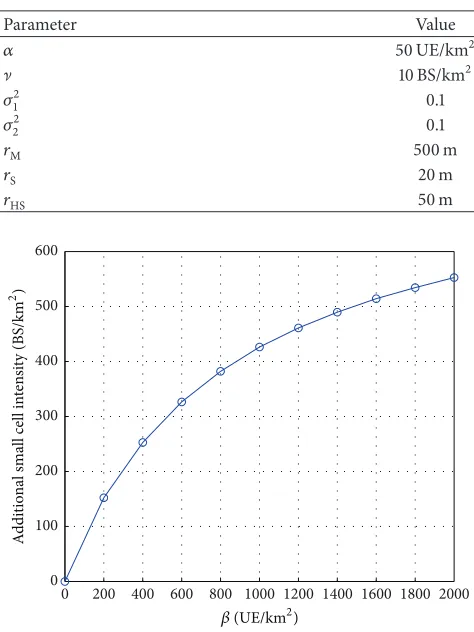
The optimization problem in (19) can be readily solved using numerical methods. Here we present numerical solu-tions of the optimal 𝜌 and 𝜇 obtained under the system parameters in Table 2. The center of the HS area is randomly generated in the macrocell coverage area while ensuring the whole HS area is within the macrocell coverage area with a minimum distance from the macrocell BS of 100 m. The intensity of additional small cells in the HS area versus the intensity of HS UE is presented in Figure 1. It can be seen that the intensity of additional small cells in the HS area increases with the intensity of HS UE at a decreasing rate. Figure 2 shows the intensity of additional small cells in non-HS areas versus the intensity of HS UE. Comparing Figure 2 with Figure 1, the intensity of additional small cells in the HS area is much higher than that in non-HS areas; the rapid increase of the intensity for additional small cells in non-HS areas when𝛽 < 1000UE/km2is because the intensity of additional small cells in the HS area is not enough to serve all the HS UE,

Table 2: System setting.

Parameter Value

𝛼 50 UE/km2

] 10 BS/km2

𝜎2

1 0.1

𝜎2

2 0.1

𝑟M 500 m

𝑟_S 20 m

𝑟HS 50 m

Additional small cell intensity in HS area

200 400 600 800 1000 1200 1400 1600 1800 2000

0

𝛽(UE/km2₎

0 100 200 300 400 500 600

A

ddi

tio

n

al small cell in

te

n

si

ty (BS/km

2 )

Figure 1: The intensity of additional small cells in the HS area (𝜌) versus the intensity of HS UE.

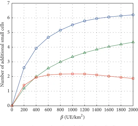
thus requiring additional small cells in non-HS area to share the extra burden caused by HS UE to the cellular network. For large values of𝛽, the intensity of additional small cells in non-HS areas decreases with𝛽, because the additional small cells in the HS area are now able to serve the majority of HS UE. Figure 3 shows the expected numbers of additional small cells in the HS and non-HS areas under the setting in Table 2.

5. Deployment of Additional Small Cells

Based on the analytical results in Section 3, we propose to maximize the average UE throughput among all UE by jointly optimizing the locations of new small cells and user associations of all cells for a HetNet affected by a HS not expected in the original network planning.

We consider the downlink (DL) of a two-tier HetNet consisting of one central macrocell and⌈𝜒_C(𝑟_M)⌉small cells randomly distributed in the macrocell coverage area. The number of existing BSs is𝑁_eBS= 1 + ⌈𝜒_C(𝑟_M)⌉. Each cell has access to the total of𝑁_RB resource blocks (RBs). Denoting the number of additional small cells to be deployed in the HS area as𝑁_NS1and the new small cells to be deployed in non-HS area as𝑁_NS2, the total number of BSs is given by𝑁_BS= 𝑁_eBS+

Additional small cell intensity in non-HS area

200 400 600 800 1000 1200 1400 1600 1800 2000

0

𝛽(UE/km2)

0 0.5 1 1.5 2 2.5 3

A

ddi

tio

n

al small cell in

te

n

si

ty (BS/km

2 )

Figure 2: The intensity of additional small cells in non-HS areas (𝜇) versus the intensity of HS UE.

Total expected number of additional small cells Expected number of additional small cells in HS area Expected number of additional small cells in non-HS areas 0

1 2 3 4 5 6 7

N

u

m

b

er o

f addi

ti

o

n

al small cells

200 400 600 800 1000 1200 1400 1600 1800 2000

0

𝛽(UE/km2₎

Figure 3: An example of the total number of new small cells under the setting in Table 2.

According to the system model in Section 2, the expected amount of HS UE is given by

𝜒_BE(𝑟_HS) = 𝛽𝜋𝑟_HS2 + (1 − 𝑒−𝑟2HS/2𝜎22)]𝜋𝑟2

HS. (21)

Let𝑁_NHS = ⌈𝐸{𝑁_U}⌉denote the amount of non-HS UE and let𝑁_HS= ⌈𝜒_BE(𝑟_HS)⌉denote the amount of HS UE in the macrocell coverage area. The set of all UE is given byN_U =

{1, 2, . . . , 𝑁U}, where𝑁U= 𝑁NHS+ 𝑁HS.

The throughput of the𝑖th UE (𝑖 = {1, 2, . . . , 𝑁_U}) is given by

𝛾_𝑖=𝑁∑BS

𝑗=1

𝑁_𝑗RB⋅ 𝑊 ⋅log₂(1 +𝑃𝑗⋅ 𝑔𝑖,𝑗⋅ 𝑢𝑖,𝑗

𝐼_𝑖,𝑗+ 𝑁₀ ) , (22)

where𝑢_𝑖,𝑗= 1if the𝑖th UE is served by the𝑗th BS and𝑢_𝑖,𝑗= 0 otherwise;𝑊is the bandwidth of a RB; without considering power control, 𝑃_𝑗 is the DL transmit power of the 𝑗th BS in a RB; and𝑃_𝑗 = 𝑃_M(S)if it is a macro-BS (small-cell BS). Assuming that the channel on each RB sees independent and identical Rayleigh fading, the channel power gain of the link between the𝑖th UE and the𝑗th BS in a RB is expressed as

𝑔_𝑖,𝑗= 𝑔_f,𝑖𝑗⋅ 𝑔_pl,𝑖𝑗, (23)

where𝑔_f,𝑖𝑗 is the exponentially distributed fading gain with unit mean and𝑔_pl,𝑖𝑗is the path loss as given in [1];𝑁_𝑗RBis the number of RBs per UE in cell𝑗and is given by

𝑁_𝑗RB= ⌊ 𝑁RB

∑𝑁U

𝑖=1𝑢𝑖,𝑗

⌋ , ∀𝑗, (24)

where, as illustrated and proven by Ye et al. in [12], equal resource allocation among the UE in all cells is optimal for the logarithmic utility; we assume that all the available RBs are allocated in each cell following the round robin algorithm with full bandwidth allocation [13], so that each cell is fully loaded and there will be intercell interference in each RB;𝑁₀ is the additive white Gaussian noise (AWGN) power; and𝐼_𝑖,𝑗 is the interference power in a RB received by UE𝑖from BSs other than BS𝑗; that is,

𝐼_𝑖,𝑗= 𝑁∑BS

𝑗󸀠_=1,𝑗󸀠 _̸=𝑗

𝑃_𝑗󸀠⋅ 𝑔_𝑖,𝑗󸀠, ∀𝑗 ∈N_BS. ₍₂₅₎

The additional small cell deployment optimization prob-lem is formulated as

arg max

U,(x1,y1),(x2,y2)

∑𝑁U

𝑖=1𝛾𝑖

𝑁_U

s.t. (x₁,y₁) ∈ 󵄨󵄨󵄨󵄨H_HS󵄨󵄨󵄨󵄨,

(x2,y2) ∈ 󵄨󵄨󵄨󵄨HNHS󵄨󵄨󵄨󵄨

𝑁BS

∑

𝑗=1𝑢𝑖,𝑗= 1, ∀𝑖 ∈NU,

𝛾_𝑖≥ 𝛾_th, ∀𝑖 ∈N_U,

𝑁RB≥ 𝑁𝑗RB> 0, ∀𝑗 ∈NBS,

𝑢_𝑖,𝑗∈ {0, 1} , ∀𝑖 ∈N_U, ∀𝑗 ∈N_BS,

(26)

the 𝑁_NS2 × 1 location vectors of additional small cells in non-HS areas;|H_HS|and|H_NHS|are the feasible deployment areas [14] for additional small cells in the HS and non-HS areas, respectively; and𝛾_th is the minimum UE throughput threshold.

Note that the joint optimization of the locations of additional small cells and the user associations of all cells in (26) is a mixed integer programming problem, which is NP-hard and requires a high computational complexity to find the global optimal solution. Therefore, we propose a practical algorithm in Algorithm 1 to solve the optimization problem in (26).

In Algorithm 1, the binary constraint of user association indicators is relaxed to 0 ≤ 𝑢𝑟_𝑖,𝑗 ≤ 1 [15]. All user association indicators are initialized as 0. Denote X₁ and X2 as the sets of additional small cells in the HS and non-HS areas, respectively. The two sets are both initialized as empty. The sizes𝑁_NS1and𝑁_NS2of vectors(x1,y1)and(x2,y2), respectively, are initialized based on the analytical results in Section 3. The optimized numbers of additional small cells to be deployed will be refined in the algorithm. The addi-tional small cells’ locations are optimized by the generalized reduced gradient (GRG) method [16].

6. Simulation Results

In this section, we present simulation results to evaluate the performance of the proposed algorithm for deploying additional small cells on top of an existing HetNet affected by HS. In the simulation, in addition to Table 2 we set the transmit power of the macro-BS and a small-cell BS as 46 dBm and 23 dBm, respectively, the bandwidth of each RB

𝑊 = 180kHz, the minimum UE throughput threshold𝛾_th=

3Mbps, the number of RBs in each cell 𝑁_RB = 50, and

𝑁₀= −174dBm/Hz.

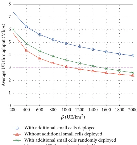
Figure 4 shows the average UE throughput with or with-out additional small cells deployed following our proposed algorithm and with the same number of additional small cells randomly deployed versus the spatial intensity of HS UE. We can see that, by deploying additional small cells following our proposed algorithm, the average UE throughput is much higher than without deploying any additional small cells or randomly deploying the same number of additional small cells. The average UE throughput can be kept above the threshold even for a very high intensity of HS UE. If without deploying additional small cells or randomly deploying the additional small cells the average UE throughput drops below the threshold as the intensity of HS UE increases, indicating that some of the UE will have unsatisfactory QoS.

In order to evaluate the load balancing performance of our algorithm, we calculate the fairness index of all UE [17] as

F= (∑

𝑁U

𝑖=1𝛾𝑖)2

𝑁_U⋅ ∑𝑁U

𝑖=1𝛾𝑖2

. (27)

The fairness index versus the intensity of HS UE is shown in Figure 5. Since the number and locations of additional small cells and user associations are optimized, the fairness index

With additional small cells deployed Without additional small cells deployed With additional small cells randomly deployed Minimum UE throughput threshold 0

1 2 3 4 5 6 7 8

A

verag

e UE t

h

ro

ug

h

p

u

t (Mb

ps)

400 600 800 1000 1200 1400 1600 1800 2000

200

𝛽(UE/km2)

Figure 4: Average UE throughput versus the intensity of HS UE.

With additional small cells deployed Without additional small cells deployed With additional small cells randomly deployed 0

0.1 0.2 0.3 0.4 0.5 0.6

F

air

ness index

400 600 800 1000 1200 1400 1600 1800 2000

200

𝛽(UE/km2₎

Figure 5: Fairness index versus the intensity of HS UE.

Initialization:

(1)𝑢𝑟_𝑖,𝑗← 0,∀𝑖, 𝑗; X1,X2← ⌀; MAX← 0; 𝑁NS1← ⌊𝜒E(𝑟HS)⌋; 𝑁NS2← ⌊𝜒D⌋

Main Function:

(2)|H_HS| ← |H|_X1 (3)|H_NHS| ← |H|_X2

(4) (𝑔,U𝑟,X∗1,X∗2) ←GRG solve (22) for X1,X2

(5) if (22) is feasible, U_𝑟∈Z+then

(6) if 𝑔 >MAX then (7) MAX← 𝑔(U𝑟, (X1,X2))

(8) U∗←U_𝑟

(9) X∗₁ ←X1

(10) X∗₂ ←X2

(11) if 𝑁_NS1= ⌊𝜒_E(𝑟_HS)⌋then

(12) 𝑁_NS1← ⌈𝜒_E(𝑟_HS)⌉

(13) return

(14) else if𝑁NS1= ⌈𝜒E(𝑟HS)⌉,𝑁NS2= ⌊𝜒D⌋then

(15) 𝑁_NS2← ⌈𝜒_D⌉

(16) return

(17) else if𝑁NS1= ⌈𝜒E(𝑟HS)⌉,𝑁NS2= ⌈𝜒D⌉then

(18) return

(19) end if

(20) else if 𝑔 ≤MAX then

(21) if 𝑁_NS1= ⌈𝜒_E(𝑟_HS)⌉then

(22) 𝑁_NS1← ⌊𝜒_E(𝑟_HS)⌋ (23) 𝑁_NS2← ⌈𝜒_D⌉

(24) return

(25) else if 𝑁NS1= ⌊𝜒E(𝑟HS)⌋,𝑁NS2= ⌈𝜒D⌉then

(26) 𝑁_NS2← ⌊𝜒_D⌋

(27) return

(28) end if

(29) return

(30) end if

(31) return MAX, U∗,X∗₁,X∗₂

(32) else if (22) is feasible, U𝑟∉Z+ then

(33) for all𝑢𝑟_𝑖,𝑗∉Z+ do

(34) 𝑔(𝑢𝑟_𝑖,𝑗= 0) →U𝑟,X1,X2, MAX

(35) 𝑔(𝑢𝑟_𝑖,𝑗= 1) →U𝑟,X1,X2, MAX

(36) end for

(37) else if (22) is infeasible, then

(38) return

(39) end if

Algorithm 1

Figure 6 shows the area spectral efficiency (ASE) [18] with additional small cells deployed following our proposed algorithm and with the same number of additional small cells randomly deployed versus the spatial intensity of HS UE. We can see that by deploying additional small cells following our proposed algorithm, the ASE is much higher than randomly deploying the same number of additional small cells, and the gain in ASE increases with the intensity of HS UE. This is because the numbers of additional small cells deployed in HS and non-HS areas are, respectively, optimized for given intensity of HS UE, as shown in Figure 3.

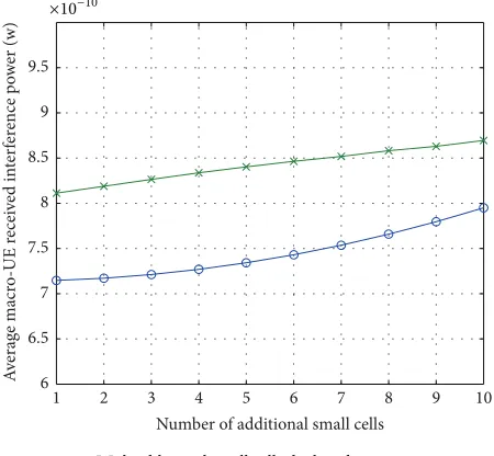
We also perform simulation to evaluate the average interference power received by a macro-UE caused by the additional small cells. The simulation result is presented in Figure 7. We can see that the average macro-UE received

interference power caused by additional small cells increases with the number of additional small cells. However, com-pared with randomly deploying the same number of addi-tional small cells, our proposed algorithm results in much less interference for any given number of additional small cells.

7. Conclusion

With additional small cells deployed With additional small cells randomly deployed 50

60 70 80 90 100 110 120 130 140 150 160 170 180 190 200

Ar

ea

sp

ec

tral efficienc

y (b

ps/H

z/km

2)

400 600 800 1000 1200 1400 1600 1800 2000

200

𝛽(UE/km2)

Figure 6: Area spectral efficiency versus the intensity of HS UE.

With additional small cells deployed With additional small cells randomly deployed

×10−10

6 6.5 7 7.5 8 8.5 9 9.5

A

verag

e macr

o-UE r

ecei

ve

d

in

te

rf

er

ence p

o

w

er (w)

2 3 4 5 6 7 8 9 10

1

Number of additional small cells

Figure 7: Macro-UE received interference power versus the number of additional small cells.

the average UE throughput (after unexpected HS occurs) by jointly optimizing the locations of additional small cells and the user associations of all cells. Simulation results show that the proposed algorithm for optimizing the deployment of additional small cells on top of an existing HetNet can guarantee the QoS requirement of all UE even for a very high density of HS UE while achieving excellent load balancing performance with a lower interference to macro-UE for the HetNet.

8. Future Work

In our future work, we plan to extend our work in two directions: (1) stochastic geometry analysis and (2) small cell deployment optimization, both considering the possible occurrence of multiple HSs (with independent HS UE inten-sities), which is closer to real HetNets. User movement and mobile traffic patterns will also be considered in the small cell deployment algorithm.

Conflict of Interests

The authors declare that there is no conflict of interests regarding the publication of this paper.

References

[1] 3GPP TR 36.912 V2.0.0, “3GPP; technical specification group radio access network; feasibility study for further advancements for eutra (release 9),” August 2009.

[2] M. Haenggi, J. G. Andrews, F. Baccelli, O. Dousse, and M. Franceschetti, “Stochastic geometry and random graphs for the analysis and design of wireless networks,”IEEE Journal on Selected Areas in Communications, vol. 27, no. 7, pp. 1029–1046, 2009.

[3] A. Babaei and B. Jabbari, “Distance distribution of bivariate Poisson network nodes,”IEEE Communications Letters, vol. 14, no. 9, pp. 848–850, 2010.

[4] H.-Y. Hsieh, S.-E. Wei, and C.-P. Chien, “Optimizing small cell deployment in arbitrary wireless networks with minimum ser-vice rate constraints,”IEEE Transactions on Mobile Computing, vol. 13, no. 8, pp. 1801–1815, 2014.

[5] W. Zhao, S. Wang, C. Wang, and X. Wu, “Cell planning for heterogeneous networks: an approximation algorithm,” in Pro-ceedings of the 33rd Annual IEEE International Conference on Computer Communications (INFOCOM ’14), pp. 1087–1095, IEEE, Toronto, Canada, April-May 2014.

[6] Y. Park, J. Heo, H. Kim et al., “Effective small cell deployment with interference and traffic consideration,” inProceedings of the 80th IEEE Vehicular Technology Conference (VTC ’14), pp. 1–5, IEEE, Vancouver, Canada, September 2014.

[7] S. F. Chou, T. C. Chiu, Y. J. Yu, and A. C. Pang, “Mobile small cell deployment for next generation cellular networks,” in Proceedings of the IEEE Global Communications Conference (GLOBECOM ’14), pp. 4852–4857, Austin, Tex, USA, December 2014.

[8] M. Tahani and M. Sabaei, “A distributed data-centric storage method for hot spot mitigation in wireless sensor networks,” in Proceedings of the International Symposium on Telecommunica-tions (IST ’10), pp. 401–408, Tehran, Iran, December 2010. [9] M. Qutqut, H. Abou-zeid, H. Hassanein, A. Rashwan, and F.

Al-Turjman, “Dynamic small cell placement strategies for LTE heterogeneous networks,” inProceedings of the IEEE Symposium on Computers and Communication, pp. 1–6, Madeira, Portugal, June 2014.

[10] T. C. Brown, B. W. Silverman, and R. K. Milne, “A class of two-type point processes,”Zeitschrift f¨ur Wahrscheinlichkeitstheorie und Verwandte Gebiete, vol. 58, no. 3, pp. 299–308, 1981. [11] J. E. Paloheimo, “A spatial bivariate poisson distribution,”

Biometrika, vol. 59, no. 2, pp. 489–492, 1972.

cellular networks,”IEEE Transactions on Wireless Communica-tions, vol. 12, no. 6, pp. 2706–2716, 2013.

[13] 3GPP TR 36.814 V9.0.0, “Evolved Universal Terrestrial Radio Access (E-UTRA); Further Advancements for EUTRA Physical Layer Aspects (Release 9),” March 2010.

[14] J. Wu, X. Chu, D. L´opez-P´erez, and H. Wang, “Femtocell exclusion regions in hierarchical 3-sector macrocells for co-channel deployments,” inProceedings of the 1st IEEE Interna-tional Conference on Communications in China (ICCC ’12), pp. 541–545, Beijing, China, August 2012.

[15] J. M. Ortega and W. C. Rheinboldt,Iterative Solution of Nonlin-ear Equations in Several Variables, vol. 30, SIAM, Philadelphia, Pa, USA, 1970.

[16] L. S. Lasdon, A. D. Waren, A. Jain, and M. Ratner, “Design and testing of a generalized reduced gradient code for nonlinear programming,”ACM Transactions on Mathematical Software, vol. 4, no. 1, pp. 34–50, 1978.

[17] R. Jain, D. Chiu, and W. Hawe, A Quantitative Measure of Fairness and Discrimination for Resource Allocation in Shared Computer Systems, vol. 38, Eastern Research Laboratory, Digital Equipment Corporation, Hudson, Mass, USA, 1984.

Submit your manuscripts at

http://www.hindawi.com

Computer Games Technology

International Journal of

Hindawi Publishing Corporation

http://www.hindawi.com Volume 2014

Hindawi Publishing Corporation

http://www.hindawi.com Volume 2014 Distributed

Sensor Networks International Journal of

Advances in

Fuzzy

Systems

Hindawi Publishing Corporation

http://www.hindawi.com Volume 2014

International Journal of Reconfigurable Computing

Hindawi Publishing Corporation

http://www.hindawi.com Volume 2014

Hindawi Publishing Corporation

http://www.hindawi.com Volume 2014

Applied

Computational

Intelligence and Soft

Computing

 Advances in 

Artificial

Intelligence

http://www.hindawi.com Volume 2014

Advances in

Software Engineering Hindawi Publishing Corporation

http://www.hindawi.com Volume 2014

Hindawi Publishing Corporation

http://www.hindawi.com Volume 2014

Electrical and Computer Engineering

Journal of Journal of

Computer Networks and Communications

Hindawi Publishing Corporation

http://www.hindawi.com Volume 2014

Hindawi Publishing Corporation

http://www.hindawi.com Volume 2014

Multimedia

International Journal of

Biomedical Imaging

Hindawi Publishing Corporation

http://www.hindawi.com Volume 2014

Artificial

Neural Systems

Hindawi Publishing Corporation

http://www.hindawi.com Volume 2014

Robotics

Hindawi Publishing Corporation

http://www.hindawi.com Volume 2014 Hindawi Publishing Corporationhttp://www.hindawi.com Volume 2014

Computational Intelligence and Neuroscience

Hindawi Publishing Corporation

http://www.hindawi.com Volume 2014

Modelling & Simulation in Engineering Hindawi Publishing Corporation

http://www.hindawi.com Volume 2014

The Scientific

World Journal

Hindawi Publishing Corporation

http://www.hindawi.com Volume 2014

Hindawi Publishing Corporation

http://www.hindawi.com Volume 2014

Human-Computer Interaction

Advances in

Computer EngineeringAdvances in

Hindawi Publishing Corporation