Joint Source-Channel Coding Optimized On End-to-End Distortion for Multimedia Source

(1)

Theses Thesis/Dissertation Collections

8-2016

Joint Source-Channel Coding Optimized On

End-to-End Distortion for Multimedia Source

Ebrahim Jarvis

Follow this and additional works at:http://scholarworks.rit.edu/theses

This Thesis is brought to you for free and open access by the Thesis/Dissertation Collections at RIT Scholar Works. It has been accepted for inclusion in Theses by an authorized administrator of RIT Scholar Works. For more information, please [email protected].

Recommended Citation

(2)

On End-to-End Distortion for Multimedia

Source

by

Ebrahim Jarvis

A Thesis Submitted in Partial Fulfillment of the Requirements for the Degree of Master of Science

in Computer Engineering

Supervised by

Associate Professor Dr. Andres Kwasinski Department of Computer Engineering

Kate Gleason College of Engineering Rochester Institute of Technology

Rochester, New York August 2016

Approved by:

Dr. Andres Kwasinski, Associate Professor

Thesis Advisor, Department of Computer Engineering

Dr. Sohail Dianat, Professor

Committee Member, Department of Electrical Engineering

Dr. Shanchieh Jay Yang, Professor

(3)

Rochester Institute of Technology Kate Gleason College of Engineering

Title:

Joint Source-Channel Coding Optimized On End-to-End Distortion for Multimedia Source

I, Ebrahim Jarvis, hereby grant permission to the Wallace Memorial Library to

repro-duce my thesis in whole or part.

Ebrahim Jarvis

(4)

Dedication

(5)

Acknowledgments

I would like to thank my advisor Dr. Kwasinki for his continuous support and help in my

research. I would also like to thank Dr. Dianat and Dr. Yang for their valuable input and

(6)

Abstract

Joint Source-Channel Coding Optimized On End-to-End Distortion for Multimedia Source

Ebrahim Jarvis

Supervising Professor: Dr. Andres Kwasinski

In order to achieve high efficiency, multimedia source coding usually relies on a use of

predictive coding. While more efficient, source coding based on predictive coding has been

considered to be more sensitive to errors during communication. With the current volume

and importance of multimedia communication, minimizing the overall distortion during

communication over an error-prone channel is critical. In addition, for real-time scenarios

it is necessary to consider additional constraint such as fix and small delay for a given bit

rate. To comply with these requirements, we seek an efficient joint source-channel coding

scheme.

In this work, end-to-end distortion is studied for a first order auto regressive synthetic

source that represents a general multimedia traffic. This study reveals that predictive coders

achieve the same channel-induced distortion performance as memoryless codecs when

ap-plying optimal error concealment. We propose a joint source-channel system based on

incremental redundancy that satisfies the fixed delay and error-prone channel constraints

and combines DPCM as a source encoder and a rate-compatible punctured convolutional

(RCPC) error control codec. To calculate the joint source-channel coding rate allocation

that minimizes end-to-end distortion, we develop a Markov Decision Process (MDP)

ap-proach for delay constrained feedback Hybrid ARQ, and we use a Dynamic Programming

(7)

(8)

List of Figures

2.1 predictive source encoder . . . 8 2.2 DPCM encoder and decoder . . . 14

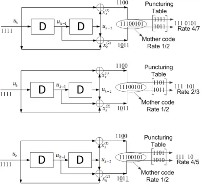
2.3 Rate-Compatible Punctured Convolutional Channel Code example. . . 18

2.4 Performance of different codes from the same family of RCPC codes with

mother code rate 1/4, memory 8 and puncturing period 8 (reproduced from [1]). . . 20 2.5 Free distance as a function of channel coding rate r for two families of

RCPC codes (reproduced from [1]). . . 21 2.6 Number of error events with Hamming weightdf as a function of channel

coding rate r for two families of RCPC codes (reproduced from [1]). . . 22 2.7 Block diagram of a joint source and channel coding scheme . . . 23 2.8 A typical end-to-end distortion curve as a function of SNR . . . 26 2.9 The single-mode D-SNR curves and the resulting D-SNR curve for a speech

source(reproduced from [1]). . . 27 2.10 The single-mode D-SNR curves and the resulting D-SNR curve for a video

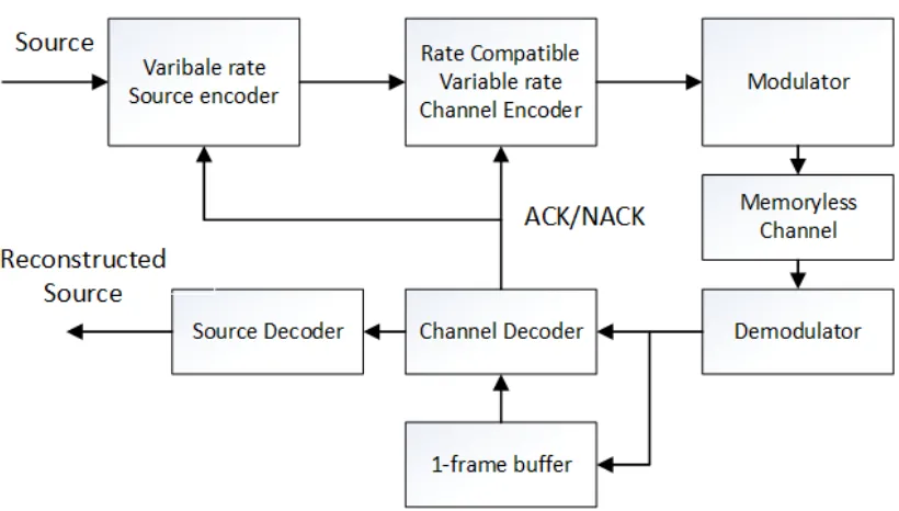
source(reproduced from [1]). . . 27 2.11 Block diagram of the communication system to implement delay-constrained

JSCC using incremental redundancy . . . 30

3.1 Gillbert Elliot channel model . . . 63 3.2 End-to-end distortion simulation of proposed work with differentα

coeffi-cients . . . 64 3.3 End-to-end distortion withα = 1coefficient . . . 65

4.1 Block diagram of DPCM coded with ARQ/FEC transmission scheme . . . 71

4.2 Markov chain of codetypes . . . 78

4.3 End-to-end distortion vs. Es/N0 for AWGN channels with and without

(11)

Chapter 1

Introduction

1.1

Motivation

The ever-growing demand for applications based on multimedia communications requires

more efficient use of communication resources. However, multimedia sources, like video,

are communication bandwidth intensive. Even though the new technology may support the

communication channels with ever-increasing bandwidth, compression of the information

source is still play an essential role in communication. This is due to the fact that with

the rate of data is growing at higher rate of bandwidth growth that force us to achieve a

more efficient bandwidth utilization. For example, in terrestrial TV broadcasting, online

gaming, virtual reality, video conferencing, satellite TV and cable TV applications, more

high-resolution video channels can be delivered within the allocated bandwidth if each

video signal is compressed for transmission. Therefore, the development of an efficient

framework to do source compression has attracted considerable research interest.

To address the multimedia source compression problem, numerous techniques have

been proposed. Predictive coding technique has shown to be highly efficient in compressing

the source data. However, there is widely spread misconception among some researchers,

who questions the performance of predictive coding over a noisy channel. They suggest

that presence of a transmission error at the decoder would cause the performance of these

(12)

To increase throughput in data transmission various transmission schemes have been

studied. Numerous studies suggest that feedback-based transmission system such as

Hy-brid ARQ with incremental redundancy can provide considerable gains in throughput over

pure (no feedback) Forward Error Control (FEC) system. This occurs because, Hybrid

ARQ system assumes there is a significant probability of correctly receiving data protected

with a weak channel code, and hence it is not necessary to add large redundancy in

ev-ery transmission. Despite these gains application of feedback based schemes to real-time

communication has been limited due to the challenges presented by inherent delay related

problems regarding transmission of incremental redundancy.

1.2

Contributions In This Thesis

The primary goal of this thesis is to address the source-channel rate allocation problem so

as to the end-to-end distortion will be minimized for the communication of a multimedia

source. First, we propose a synthetic source that abstracts the fundamental components of

video. This is because, working with video is difficult due to complexity of source model.

Furthermore, in the proposed source, we assume that the first sample is memoryless and

the rest is DPCM coded using the memory between the samples. The precise and novel

mathematical expressions have been used to indicate the end-to-end behavior of such

sys-tem. Furthermore, our simulation results show that the performance of predictive coders in

the presence of errors not only will not be catastrophic but also with the proper use of error

concealment it leads to having the same performance as the memoryless system. Second,

we address the joint source-channel rate problem in the incremental redundancy Hybrid

(13)

from modeling our problem with a Markov Decision Process (MDP). A Dynamic

Program-ming algorithm is used to find the optimal source and channel rates. Our simulation results

(14)

Chapter 2

Background

In this chapter, we discuss various technologies and techniques relevant to this work. The

chapter is divided into five parts. First, we will briefly introduce previous studies that deals

with similar problem. Then we study the basic structure of predictive coding. In Section

2.2.3 we will investigate the statistical properties of the source. Then, we focus our study on

differential pulse code modulation (DPCM). We also describe the overall features of DPCM

encoder and decoder. In third part of this chapter we will discuss the idea behind variable

rate codes. We describe the channel model and decoding mechanism, recognizing that

understanding the performance of such system is essential to design joint source-channel

codes. In the fourth part of this chapter, we extend the study of RCPC codes, and look

into joint source-channel coding. In the last part of this chapter, we discuss the use of

incremental redundancy bits in the joint source-channel coding system.

2.1

Previous Work

Of the works with similar objective as ours, the work most closely related to this thesis is

that by Chou et al. [2], which addresses the problem of streaming packetized media over

a lossy packet network by rate-distortion optimization. Assuming that each data unit of

the video stream is independent of one another, the authors showed that the problem of

(15)

optimization for a single unit data. Furthermore, the authors derived a practical algorithm

to address a variety of transmission scenarios such as sender driven or receiver driven

trans-mission, and streaming over the best effort network. This algorithm used a Markov decision

process framework, where the cost-error model differentiate different transmission

scenar-ios from each other. The expected rate-distortion optimization was done by using a general

iterative algorithm to form a convex hull that can be solved by Lagrange multiplier

opti-mization technique. Furthermore, authors assume a fix short delay (up to several seconds)

in the beginning of the data transmission that is independent of the length of the

presenta-tion. In addition, their rate optimization system is primarily based on the usage of buffer

and playback on the receiver side, where incremental redundancy can be more suitable for

a more constrained delay and buffer space. By considering the distortion that is suffered by

each single data unit independent of each other and developing an error-cost model based

on each frame, concluding the optimal rate-distortion will be approximation of the optimal

scenario (scenario that studies the affect of error on current frame to the future frame).

The work [3], studies the performance of DPCM predictive coding method under an

error prone channel. This research shows that DPCM works reasonably well to compress

the signal. However, the performance degrades considerably when errors occur during

transmission. The authors concluded that this is due to error propagation at the decoder,

which originates from the DPCM mechanism that relies on previous samples at decoder.

The authors suggest that this leads to a catastrophic performance with the even single error

during transmission. Furthermore, this study showed that a low-rate feedback channel

would improve the overall performance.

The work of Kwasinski et al. [4], presented a joint-source channel coding scheme based

(16)

under strict delay constraints. The proposed scheme works with a constant bit rate and

de-lay (one frame dede-lay). In order to add incremental redundancy to the frame when its coded,

the source is encoded with a lower bit rate. The underlying design technique uses a Markov

chain by introducing various code types, where each code type describes the different

com-positions of the frames. In the work, there are three possible outcomes to a transmission.

The authors assumed three successively transmitted frames, referred in time as previous,

current and next frames, and the corresponding source blocks as previous, current and next

source blocks. The feedback-based transmission scheme is described as, when the previous

block is received with errors, the current block will contain the codeword for the current

frame and incremental redundancy for the previous one and will lower the channel code

rate when possible (the maximum number of different code rates not reached). If the

cur-rent block was received without errors after channel decoding, then the curcur-rent frame will

consist entirely of the current frame’s bits without incremental redundancy. The result of

the work [4], showed distortion value decrease compare to no feedback transmission and

hence,28%increase in the simultaneous calls that can be supported on the CDMA network.

In [5], Zhihai He et al. shed more light on the source and channel distortion

model-ing. The authors developed a rate-distortion model for DCT-based video by considering

the macroblock intrarefreshing rate. Using this R-D model, the authors estimated the

dis-tortion given the bit rate and intrarefreshing rate. Furthermore, in this work the behavior of

channel error on video coding and transmission is described through closed form

expres-sions. However, the accuracy of their distortion estimation is largely based on the size of

(17)

2.2

Predictive Coding

A data compression system could be translated into any scheme that operates on source

data to eliminate possible redundancies so that only those values needed to reproduction

are preserved. There are two main approaches to address redundancy issues namely, time

and frequency domain techniques. In the first category, compression is performed through

prediction of source samples by exploiting the fact that source samples are serially

corre-lated. Therefore, predictive coding system codes the difference between the source sample

and the predicted value instead of coding the source. Common time domain coders include

differential pulse code modulation (DPCM) and delta modulation (DM). In frequency

do-main methods, first, the source spectrum is divided into several frequency bands through

subband filtering. Then a procedure called frequency decomposition is applied. This is

fol-lowed by assigning quantizers to the subbands. If we increase the number of the subbands,

we will get less correlation between the subband. Wavelet, subband, and transform coders

such as traditional JPEG, MPEG- 1, MPEG-2, H.261, H.263, and H.265 are standard for

frequency-based domain coding. Scalar quantization of each source sample independently

is a suboptimal method, when there is time correlation between samples. The correlation in

time between samples may appear as two samples that are close in time show little change

in value. Speech and audio sources both show time correlation between samples because

the physical mechanism by which they are generated create a signal that changes smoothly

over time. The same can be expressed about image and video sources for time and spatial

correlations. When two neighbor samples are correlated, one can use the quantized

infor-mation from one sample and reduce the amount of data needed to code the other one.

One of the methods that exploit the correlation between samples (memory) is predictive

(18)

[image:18.612.100.515.94.187.2]

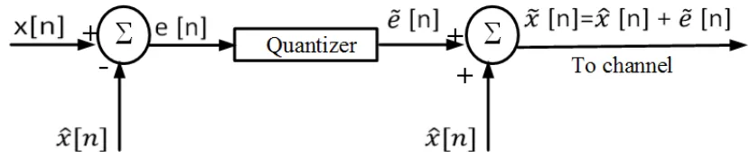
Figure 2.1: predictive source encoder

the source sample x[n]before quantization. The same quantity is added to the quantized difference ˜e[n] to generate the reconstructed output x˜[n]. An important property of pre-dictive coding is that the reconstruction error equals the quantization error. The following

equations prove this fact:

e[n] = x[n]−xˆ[n]

˜

x[n] = ˜e[n] + ˆx[n]

x[n]−x˜[n] = e[n] + ˆx[n]−(˜e[n] + ˆx[n])

= e[n]−˜e[n]. (2.1)

The best choice of predicted value as notedxˆ[n]in the figure 2.1, to produce a difference

e[n], can be yield using two main methods namely, maximum a priori probability (MAP) and linear minimum squared estimate (LMMSE). MAP obtainsxˆ[n]from a group of neigh-boring samples. Let us denote the adjacent samples by g[n]. The MAP estimatexˆ[n]of

x[n]is given by,

ˆ

x[n] =arg maxxp(

(19)

The optimization solution calculated by MAP is often considered as too slow due to the

complexity and number of operations so that one may take into account a suboptimal

set-tlement to this problem. In the case of adjacent samples in the source sequence showing

high dependency (strong correlation), the simplest solution is the previous samplex[n−1]. Note that under this condition the difference e[n] = x[n]−x[n −1] is most likely to be small. The main issue with MAP is that to predictx[n]the solutionx[n−1]does not take into consideration the correlation between samples.

As mentioned to estimatex[n]we can use the linear minimum squared estimate (LMMSE). This method uses a linear combination of samples in the neighbor groupg[n]. The follow-ing section will review the design of the optimal LMMSE for an autoregressive source as

will be considered in this thesis.

2.2.1 Optimal Linear Prediction for Autoregressive Sources

From [6], let...., x[−1], x[0], x[1], x[2], .., x[n]be a zero mean, stationary source sequence. The linear prediction ofx[n]from the pastLsamples can be implemented as,

ˆ

x[n] = L X

k=1

akx˜[n−k], (2.2)

where a1, a2, ..., aL are the prediction filter coefficients. The solution that minimizes the

MSE E

ˆ

x[n] −x[n]2

for the vector of prediction coefficients a∗ = (a1∗,a2∗, . . . ,aL∗),

comes from the orthogonality principle [7] that the errorx[n]−xˆ[n]should be orthogonal to the past sample values,

E

(x[n]−xˆ[n])x[n−k]

(20)

The orthogonality principle generates the Yule-Walker equation [6],

φx(L)a∗ =φx, (2.4)

where in 2.4,φx(m) =E[x[n]x[n−m]]is the autocorrelation function of the source with

different lag m, m = 1,2, ..., L; andφx = (φx(1), φx(2), ..., φx(L))T. Then for the L-th

order autocorrelation matrix of the source we have,

φx(L) ={φ(|k−m|)}L −1

k,m=0. (2.5)

We can express 2.4 in an expanded form of the Yule-Walker that shows the individual

elements as          

φx(0) φx(1) . . . φx(L−1)

φx(1) φx(0) . . . φx(L−2)

..

. ... ... ...

φx(L−1) φx(L−2) . . . φx(0)           ×          

a∗₁ a∗₂

.. .

a∗_L

          =          

φx(1)

φx(2)

.. .

φx(L)          

The MMSE can be described as,

e2_min = min E[|x[n]−xˆ[n]|2_]

= φx(0)−φTxa0

= φx(0)−φTx(φ(xL)) −1_φ

x (2.6)

Note that thee2_min is always less thanφx(0)since the autocorrelation matrixφL is always

non-negative definite. This condition will assure that the inverse (φ(xL))−1 is also definite

positive thenφT_x(φ(xL))−1φx >0for any vector φx. Therefore, the minimum error variance

(21)

2.2.2 Source Key Properties

To study the source statistical properties, we are assuming the input source x[n]follows a first autoregressive, AR(1), source model, we can express the source model as,

x[n] =ρx[n−1] +z[n], (2.7)

where the innovation process z[n] forms a sequence of independent and identically dis-tributed random-valued samples following a Gaussian distribution with zero mean and

variance σ2

z. The source probability distribution follows a first-order Markov

(Markov-1) process, since the current random variable x[n] only depends on the previous sample

x[n−1]and the innovation processz[n]and it does not depend on other past samples. The source is encoded by operating on blocks ofMsamples{x[0], x[1], . . . , x[M−1]}. We assume the first sample (x[0]) is encoded using a memoryless source encoder and the rest of samples are encoded using predictive coding encoder (DPCM). This mechanism

models the main components of the video encoder. In the video encoder the first frame

in a block of frames is encoded independent from other frames and without considering

the time-correlation (as I frame), and the rest of the frames are encoded by exploiting the

temporal correlation with the previous frames (as P frames). Following a simplified model

for motion compensated video coding, the first sample is encoded at a rate R0 bits per

sample using a scalar memoryless encoder and all subsequentM−1samples are encoded using a DPCM encoder with a rate ofRnbits per sample for samplex[n]. Note that through

(22)

samples only:

x[n] = ρx[n−1] +z[n]

= ρ(ρx[n−2] +z[n−1]) +z[n]

= ρ2x[n−2] +ρz[n−1] +z[n]

= n X

j=0

ρjz[n−j]. (2.8)

Since x[n] = Pn j=0ρ

j_z_[_n₋_j_]_{, a linear combination of Gaussian random variables,} _x_[_n_]

is also Gaussian. This is, x[n] ∼ N(0, σ2

x). From this result, we can now calculate the

expected value forx[n],

E[x[n]] =Eh

n X

j=0

ρjz[n−j]i= n X

j=0

ρjE[z[n−j]] = 0 (2.9)

(23)

samplesx[n] =P∞_j₌₀ρj_z_[_n₋_j_]_{. In this case, the autocorrelation is}

φ(k) = E[x[n]x[n−k]]

= E

h_X∞

i=0

ρiz[n−i] _X∞

j=0

ρjz[n−k−j] i = ∞ X i=0 ∞ X j=0

ρi+jE[z[n−i]z[n−k−j]]

(#) =

∞ X

j=0

ρk+2jσ_z2

= ρkσ_z2

∞ X

j=0

ρ2j

= σ2_z ρ

k

1−ρ2,

where equality (#) follows because the innovation process samplesz[n]are uncorrelated,

Ehz[n−i]z[n−k−j]i =       

σ_z2, ifi=k+j,

0, otherwise.

(2.10)

Now, since by definitionσ2

x=φ(0), it follows that

σ_x2 = σ 2 z

1−ρ2. (2.11)

Therefore, the covariance of the source can be expressed as,

φ(k) =σ_x2ρk, k≥0. (2.12)

Using this result and that the autocorrelation function is even, it follows that

(24)

[image:24.612.176.438.94.349.2]

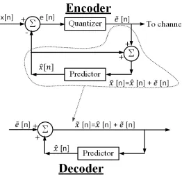
Figure 2.2: DPCM encoder and decoder

Finally, we can conclude thatx[n]∼ N 0, σ_z2/(1−ρ2), ρ≥0.

2.2.3 DPCM System Description and Statistical Overview

The principle of differential pulse code modulation (DPCM) is based on ideas from

predic-tive coding. DPCM was first introduced in [8] to improve the efficiency of communication

systems by taking advantage of the correlation between the source samples. DPCM is a

compression method which is even today widely used. Where other compression methods

may offer better compression ratio, DPCM offers simplicity results in low cost

implemen-tation, which is highly efficient especially in high speed compression.

Figure 2.2, shows the architecture of the DPCM encoder and decoder. It can be seen

that the DPCM main components are comprised of two main components: predictor and

(25)

sourcex[n]and a predicted valuexˆ[n], then it quantized to˜e[n], which is then transmitted to the destination. The predicted value xˆ[n]is obtained from a linear combination of the pastLvalues of the sourcex˜[n−1], . . . ,x˜[n−L], which are derived frome˜[n]accordingly. As a result, the current reconstruction ofx˜[n]is the sum of the predicted valuexˆ[n]and the quantized prediction residual˜e[n]. Note that the reconstruction error can be yield the same way as discussed in predictive coders in (2.1).

As Figure 2.2 illustrates, DPCM uses a linear prediction filter with the input-output

relation given by,

ˆ

x[n] = L X

k=1

akx˜[n−k], (2.14)

for a predictor of order L with coefficients ak. In the particular case of a first order

au-toregressive, AR(1), source,L = 1and we havexˆ[n] = a1x˜[n−1]. From (2.7), it is well

known ([6]) that to minimize the mean square prediction error the coefficientashould be,

a =ρ, making the optimum linear predictor bexˆ[n] =ρx˜[n−1].

The main challenge for DPCM comes from the fact that the prediction is made from

the past values which are not available at the destination because their reconstructed values

contains error. If the predictor works by storing the past M values in the memory and the destination tries to reconstruct the samples, the reconstruction error will accumulate.

Therefore the DPCM predictor at encoder side uses the source reconstructed values which

are the same as those at the destination.

2.2.4 DPCM Coding Error and Gain

The prediction residuals (e[n]) are a scalar source signal, with values quantized indepen-dently of each other, as shown in Figure 2.2. In DPCM linear prediction is obtained similar

(26)

squared value of the prediction residual and is closely related to the variance of the source.

However, the coding error for DPCM is not the same value as the e2_min in (2.6), since in DPCM the prediction method is done differently. In (2.6), the prediction takes place on the

actual past values while in DPCM it takes place on previously reconstructed values.

If we assume that the transmission is done at high rates while the quantization error

is small then we can approximate that the predictor coefficients are calculated using the

source covariancesEx[n]x[n−l], l = 0,1, . . . , L. Alsoxˆ[n], is approximately derived from the same past values. Using this approximation the coding error can be approximates

as [6],

Ehˆe[n]2i ≈φx(0)−φTx(φ (L) x )

−1_φ

x. (2.15)

The gain in DPCM coding over PCM can be defined as,

GDP CM/P CM =

DP CM

DDP CM

. (2.16)

Which is derived from the ratio of the their corresponding coding errors. Since they both

have the same unit variance distortion versus rate function the ratio will be the ratio of their

source variance which is,

GDP CM/P CM =

φx(0)

φx(0)−φTx(φ (L) x )−1φx

. (2.17)

Note that the gain will be more than one in the case of the source with memory.

2.3

Rate-Compatible Channel Codes

Rate-compatible channel codes offer flexibility in adapting the channel code rate when it

is used for joint-source channel coding applications. This is because in these applications

(27)

codes, the members are derived from the lowest rate code which is called the ”mother

code”. The higher rate codes in the rate-compatible family can be encoded using puncture

tables that operates on the mother code. For each RCPC code, there is a puncturing table

to determine the bits that are being removed from the output of mother code encoder. The

puncturing table consists of rows which related to each output encoder and columns that

show the order of bits. The zero element in the table means that bit from the mother code

to be punctured and one indicates that the mother code in that position not to be punctured.

Note that since the number of columns are limited, the puncturing operation is repeated

periodically. The length of this repetition is called the puncturing period for RCPC codes.

The rate compatible restriction over puncturing table ensures that all code bits of high rate

codes are used by lower rate codes. If we express that the mother code is extended by

puncturing a low rate _N1 with period P anda as the punctured matrix andl as the matrix sequence number, latter restriction can be expressed as,

if aij(l0) = 1 then aij(l) = 1 for all l ≥l0 ≥1, (2.18)

or equivalently,

if aij(l0) = 0 then aij(l) = 0 for alll≤l0 ≤(N −1)(P −1). (2.19)

Rate-compatible channel codes can be constructed from any linear code, but it is more

efficient and straightforward when based on the use of convolutional codes in which case

they are called rate-compatible convolutional codes (RCPC).

Figure 2.3 shows an example of generating various coding rates using the same

convo-lutional code. The figure shows three codes are derived with coding rates decreasing from

(28)

[image:28.612.105.517.191.572.2]

(29)

the zero puncturing we get the rate which is equal to the rate of the mother code and any

positive number of puncturing results in higher coding rate compare to the mother code.

The top code has the largest rate in the example of Figure 2.3 at 4/7, and is derived from puncturing one bit out of four bits. The punctured bit corresponds to an entry of zero in

puncturing table corresponding to the output of the bottom line of the encoder. The deleted

bit is shown as underlined. For the example of the top code in Figure 2.3, the puncturing

table is,



 

1 1 1 1

1 0 1 1 

 

where it can be seen that the punctured bits are the second, sixth, tenth, etc. The puncturing

period here is four.

The decoding of RCPC codes can be done the same way as the other punctured

convo-lutional codes. As a matter of fact, the common way of implementing the decoder is to use

Viterbi decoder. As it is discussed in [9], the soft decision Viterbi algorithm can be utilized

for decoding all the RCPC codes with various puncturing rules.

2.3.1 Performance of RCPC Codes

The performance of RCPC codes can be calculated in the same way as other convolutional

codes. Therefore, it can be measured based on the probability of making a decoding error.

The applied puncturing rules will affect the strength of the code. Higher rate codes are

weaker regarding correcting errors. This point is shown in Figure 2.4, where the BER is

plotted as a function of channel SNR for different RCPC codes from the same family.

The analysis of the performance of RCPC codes depends on the channel model and

decoding mechanism, since they affect the probability of making a decoding error. It was

(30)

[image:30.612.115.488.228.524.2]

(31)

[image:31.612.134.487.97.250.2]

Figure 2.5: Free distance as a function of channel coding rate r for two families of RCPC codes (reproduced from [1]).

metric Viterbi decoder. Assuming, that the input to the encoder is the all zero sequence.

The probability of making a decoding error is calculated as the probability of not choosing

the right path (all zero in this case) in the corresponding trellis diagram of the decoder.

Note that the input can be a stream of bits with not a fixed length necessarily. Therefore,

the performance is measured as the probability that the path which separates and rejoins all

the zero path for the first time has a path metric larger than the all zero path. This problem

can be related to calculating the probability that the Hamming distance between one path

and the zero path isd. According to [1], this probability can be expressed as,

Pe(d|γb) = 1 2 erfc

p

drγb, (2.20)

where ris the channel code rate, γb = Eb/N0 is the received SNR per bit and erfc (γ) is

the complementary error function defined as,

erfc(γ) = 2/π

Z ∞

γ

e−u2du. (2.21)

(32)

[image:32.612.128.489.96.247.2]

Figure 2.6: Number of error events with Hamming weightdf as a function of channel coding rate r

for two families of RCPC codes (reproduced from [1]).

distance asdf, the upper bound probability of decoding error can be written as,

P(γb)≤ ∞ X

d=df

a(d)Pe(d|γb), (2.22)

wherea(d)is the number of paths with Hamming distance dfrom the all zero path. Note that in RCPC codes both danda(d) depends on the channel code rate. Figure 2.5 shows this relation in more detail where the free distance decrease with increasing in channel code

rate. This observation can be expressed as,

df =ke−cr, (2.23)

wherekandcare constants. Figure 2.6 illustrates the fact that the behavior of the function

a(d)can not be approximated as a simple function of channel coding rate (r).

Finally, as we shall see in section 2.4, rate compatible channel codes, by providing a

simple mechanism to adapt channel coding rate while using the same decoder, they are very

useful when implement joint-source channel coding techniques. Specifically, in the case of

(33)

[image:33.612.96.519.90.149.2]

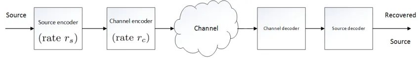
Figure 2.7: Block diagram of a joint source and channel coding scheme

other words, we tend to transmit the source bits with the highest channel rate, where the

SNR is high. Using this method in conjunction with the technique that is called

“Incremen-tal Redundancy” results in efficient multimedia communication. Incremen“Incremen-tal redundancy

transmission scheme heavily relies on the use of flexible channel codes. Incremental

re-dundancy technique will be discussed in more detail in section 2.5.

2.4

Joint Source-Channel Coding

Shannon’s source-channel separation theorem states that, in point-to-point communication

systems, source coding (compression) and channel coding (error protection) can be

per-formed separately and sequentially, while maintaining optimality. In many practical

appli-cations, the conditions of the Shannon’s separation theorem can not be used. This is due to

the optmality condition remains true only in the case of asymptotically long block lengths

of data. Thus, significant interest has developed in various schemes of joint source-channel

coding.

The most shared and simple way to design a joint source-channel coding system is by

implementing each source and channel separately while configuring them to work jointly

together. In this approach, called concatenated joint source and channel coding we

con-nect separate source and channel coding blocks serially but their operating parameters are

jointly optimized. As figure 2.7 shows, while, the source and channel encoding blocks are

(34)

parameters as a single coding unit. Then for this purpose, the source and channel codes are

chosen such that they can be easily modified. Two of the common mechanisms employed

are embedded source codecs and rate-compatible punctured channel codecs.

The primary goal in designing a concatenated joint source-channel is to assign a proper

rate to the channel and source encoder. The resource allocation for joint source and the

channel coding is done for a given channel signal to noise ratio (SNR). In addition, it is

assumed that the total number of bits transmitted through the channel is fixedW bits. The main goal regarding the joint allocation of the source and channel coding rate is

to minimize the end-to-end distortion. The end-to-end distortion is the combination of the

source coding distortion and the channel-induced distortion. Source coding distortion is

related to the quantization and compression processes, and channel-induced distortion is

caused by channel errors that occur during transmission and cannot be corrected by the

channel coding process. As such, the end-to-end distortion can be mathematically written

as,

D(rs, rc, γ) =DFPr(γ) +DS(rs)

1−Pr(γ)

, (2.24)

where rs is the source encoding rate measured in bits/sample, rc is the channel coding

rate, γ is the channel SNR, DF is the total distortion when an error occurs during

trans-mission and cannot be corrected by the channel code, Pr(γ) is the probability of having

post-decoding channel errors andDS is the source encoding distortion.

Note that in (2.24), the possibility of not having an error during transmission is 1−

Pr(γ), in which case the end-to-end distortion is equal to the source encoding distortion

DS(rs) only. When an error happens in the channel during transmission and the channel

(35)

lost information needs to be estimated or concealed by an error concealment mechanism.

In this situation, the distortion introduced is the sum of the source distortion, and

channel-induced distortion denoted asDF.

The distortionDF value is usually observed to be much larger than DS, and it is

re-lated to various variables, including the level of compression, the algorithm used for error

concealment and the source statistics. In some cases the value ofDF can be derived from

statistical considerations. In the absence of any extra information, it is known that the

op-timal error concealment consists of replacing the lost source samples with their expected

value. In the case of a memoryless Gaussian source with zero mean, the error concealed

value isˆs=E[s] = 0andDF is,

DF =E h

(s−ˆs)2 i

= 1. (2.25)

The quality of communication perceived by the end user depends on the reconstructed

sam-ples at the receiver side, which also rely on the overall end-to-end distortion. To receive a

better quality, then, the goal is to minimize the end-to-end distortion by appropriate choice

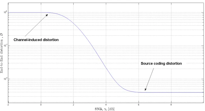
of source coding rate(rs)and the channel coding raterc. Figure 2.8 illustrates the typical

plot of the end-to-end distortion as a function of channel SNR. It can be observed in

Fig-ure 2.8, that when the channel SNR is high, the probability of post channel decoding error

(Pr(γ)) is very low, close to zeroPr(γ)≈0, and the value ofD(rs, rc, γ), using (2.24) can

be expressed as,

D(rs, rc, high γ)≈DS(rs). (2.26)

(36)

[image:36.612.136.487.101.291.2]

Figure 2.8: A typical end-to-end distortion curve as a function of SNR

value of the end-to-end distortion will be,

D(rs, rc, low γ)≈DF. (2.27)

It can be seen that between the high and low SNR regions there is a transition, whereby

decreasing the SNR value the end-to-end distortion value will increase from DS(rs) to

DF. Since the total transmitted bits are fixed then by decreasing the SNR, we have the

situation where the number of uncorrected errors increases. Figure 2.9 and 2.10, illustrate

the typical results when plotting the end-to-end distortion as a function of channel SNR.

These figures provide insight into the basic trade offs associated with joint bit rate allocation

for concatenated JSCC. The mechanism linking source and channel coding rate implies that

choosing a smaller channel coding rate will result in adding more redundancy and having

(37)

[image:37.612.128.489.142.294.2]

Figure 2.9: The single-mode D-SNR curves and the resulting D-SNR curve for a speech source(reproduced from [1]).

Figure 2.10: The single-mode D-SNR curves and the resulting D-SNR curve for a video

[image:37.612.131.486.456.603.2]

(38)

The source and channel coding rates in concatenated joint source-channel coding are

jointly chosen for a given SNR value. In a practical scenario, the possible choices for

cod-ing rates are selected from a finite number of discrete choices. Letrs ={rs1, rs2, . . .}and

rc ={rc1, rc2, . . .}, andΩ = {Ωi}, be the finite set that defines possible source encoding

rates, possible channel encoding rates and all possible working combination of source code

rate and channel code rate as operating mode, respectively. Since the total number of bits

are fixed (W), the source and channel rates only are one independent variable, since they are relates as,

W ≥N rs/rc, (2.28)

where N is the number of source sample at the input of the source encoder during one encoding period. The inequality (2.28), provides us with numerous choices for the value of

rs given a fixedrc, but only the largest possible value is reasonable, because given a fixed

SNR, the value of Pr(γ)is also fixed, so the largest possiblerswill minimize theDS(rs)

and end-to-end distortion. Therefore, the choice of rs givenrc is the one where (2.28) is

closest to an equality. Consequently, the operating mode can be identified through only the

choice of rc or the choice ofrs. In practice since we are working with discrete numbers,

this condition may not exactly meet, and some padding bits may be added. If we define the

operating mode by the source coding rate we have, Ω = {Ωi} = {rsi}, then the equation

(2.24), will change notation accordingly to the following,

dΩi =DFPΩi(γ) +DS(Ωi)

1−PΩi(γ)

, (2.29)

where PΩi(γ) is the frame error probability for the given operating mode (Ωi), DS(Ωi)is

the source codec D-R function, and DF is the distortion when an error happened during

(39)

end-to-end formula (2.29) is called the single mode D-SNR curve, since for each mode we

have a different D-SNR curve.

The goal of concatenated joint source-channel coding design is to find the operating

mode that minimizes the end-to-end distortion. Mathematically, this goal can be defined

as,

min Ω

DFPΩi(γ) +DS(Ωi)

1−PΩi(γ)

,

such that W ≥N rs/rc.

The optimization problem for a range of channel SNRs forms an overall minimum

distor-tion funcdistor-tion that is called the “D-SNR curve”. This optimization problem is discussed in

more detail in chapter 4.

2.5

Delay-Constrained JSCC using Incremental Redundancy with

Feed-back

Studying delay-constrained joint source-channel coding is motivated by the ever

increas-ing demand over sendincreas-ing real-time multimedia sources with constrained delay. As it is

described in [10], delay-constrained video coding applications requires a total delay, which

consists of buffer delay and transmission delay, to be smaller than the interval between two

frames. This results in using Forward Error Correction (FEC) as the primary method for

error control.

Figure 2.11 illustrates the block diagram of the communication system to implement

delay-constrained JSCC using incremental redundancy. The source encoder works on a

(40)

[image:40.612.117.527.83.316.2]

Figure 2.11: Block diagram of the communication system to implement delay-constrained JSCC using incremental redundancy

fixed number of bits are generated to encode the source samples. These bits form source

blocks. In the next step codewords are generated from source blocks using a concatenation

of an outer error detection code and an inner error correction code selected from a rate

compatible family of codes.

Since the transmission is synchronous over a wireless channel, it can be assumed

fixed-size frames per source block sample. Incremental redundancy is used with feedback based

transmission mechanism. The transmission system uses ACK/NACK feedback to

deter-mine what codewords should be included in a frame. A frame may contain codewords and

partial codewords for one or two source blocks depending on the feedback.

To see the operation of the system in Figure 2.11, let’s consider three frames in three

consecutive time-frames regarded as previous, current and next frames with

correspond-ing source blocks followcorrespond-ing the same sequence in time. If the feedback received at sender

(41)

to codewords of the current source block. At the receiver, the current frame will be

de-coded to retrieve the current source block. The channel coding operation determines the

success or failure of this transmission and will send one bit ACK/NACK through a

feed-back channel to notify the sender. If the sender receives an ACK for the current frame, it

would continue sending the next frame with the same operation as for the current frame.

If a NACK is received, which indicates the failure during transmission of a current frame,

the channel encoder would choose lower rate channel code for the current source block

(can be achieved through rate compatibility of channel codes by adding extra parity bits).

These extra parity bits, referred to as Incremental Redundancy bits, are sent as a part of

the next frame combined with the codeword for the next source block. Because the frame

size is fixed, the source and channel coding rate in the next frame will be chosen so as to

accommodate the incremental redundancy for the current source. On the receiver side, the

decoder will decode the next codeword and also will try to decode the current codeword

to the best of its capability by combining the previously received source block and the

re-ceived incremental redundancy. Note that upon receiving the incremental redundancy the

currently decoded source block is accepted without further attempts at using incremental

redundancy. Thus, the maximum delay, in this case, will be one frame to decode a source

block which is in compliance with the condition mentioned in [10]. Note that, in this

mechanism the essential property is to reduce the source encoding rate in the next frame, to

allow for the transmission of incremental redundancy bits to help error recovery of the

cur-rent source. As a result, the decoded next source block may suffer higher average distortion

than the current source. However, it will help to decode the current source and reduce its

channel-induced distortion.

(42)

is discussed in chapter 4.

2.6

Summary

In this chapter, we have summarized the elements of predictive coding system and focused

on DPCM as an instance of such a system. Then we described the source fundamental

properties. Also, we considered the performance of DPCM through end-to-end

distor-tion that is the combinadistor-tion of source encoding distordistor-tion and channel-induced distordistor-tion.

To address the channel-induced distortion we studied the rate-compatible channel codes.

Then, to optimize the overall end-to-end distortion we used RCPC codes in conjunction

with joint-source channel coding. Finally, we highlight the importance of the incremental

redundancy when designing a system based on the delay-constrained joint source-channel

(43)

Chapter 3

Distortion Analysis

3.1

Problem Setup

Because multimedia sources usually exhibit some form of correlation between samples,

the source codecs are frequently built around a DPCM-type codec, where the correlation of

source samples is exploited through the use of predictive coding. However, it has become

a broadly spread notion that transmission errors significantly degrade the performance of

DPCM-type codecs (e.g. [3]). Yet, in an often overlooked comment in [11], this notion

is noted as a misconception. Nevertheless, this misconception persisted after [11], maybe

because this is only a passing comment within a section that is focused on an analysis

that does not provide the full insights into the mechanism at play. In fact, the comment

in [11] made no attempt at presenting an unequivocal case to dispel the misconception by

not going any further than a single comment and not conducting any study about when

transmission errors significantly degrade the performance of DPCM-type codecs and when

this is not the case. In this chapter we present an analysis that leads to a closed-form

expressions to characterize the main elements that determine the end-to-end distortion of

multimedia codecs, allowing for an in-depth study of the effects of transmission errors.

To achieve this, we extract and model the core operational elements in multimedia source

codecs by focusing on a simpler DPCM-based source coding scheme. The insight from

(44)

experience the same distortion due to transmission errors, even when DPCM-type codecs

suffer from error propagation while memoryless codecs do not. Furthermore, the analysis

will show that the reasons for this result are the DPCM coding gain and the better error

concealment performance that are achieved in a DPCM system by exploiting the source

memory and by using the optimal predictor in the DPCM coding loop.

The rest of this chapter is organized as follows, section 3.2, describes the problem and

the setup used to study the problem. Section 3.3 derives the equations related to source

encoding distortion. Subsection 3.4 leads to formulate the end-to-end distortion followed

by discussion and numerical results.

3.2

System Setup

In order to mimic the main configuration of multimedia codecs, we study the end-to-end

distortion of a communication system that transmits a block of M samples using a mem-oryless source encoder for the first sample and a DPCM (predictive coding) encoder for

the rest of samples. This setup models the main elements in the encoding of video, where

the fist frame in a block-of-frames is encoded without exploiting the source sample

time-correlation (making it an I-frame), and the encoding of the rest of the frames can use the

temporal correlation with previous frames (as P frames). The considered DPCM encoder

and decoder are shown in Fig. 2.2, wherex,xˆandx˜are the source, predicted and decoded samples respectively. We will assume a synthetic source that is designed to instantiate the

most fundamental characteristics of a video-like source. As such, we assume a source that

follows a first order autoregressive - AR(1) - process: x[n] = ρx[n −1] +z[n], where the innovation process z[n] forms a sequence of independent and identically distributed random-valued samples following a Gaussian distribution with zero mean and varianceσ2

(45)

Accordingly, A DPCM uses a linear prediction filter with the input-output relation given

by,

ˆ

x[n] = L X

k=1

akx˜[n−k],

For a predictor of orderLwith coefficientsak. In the particular case of a first-order

autore-gressive, AR(1), source,L= 1, and we have,

ˆ

x[n] =a1x˜[n−1]. (3.1)

From ([6]), it is well known that to minimize the mean square prediction error,a=ρ. Note that the source statistical properties show the same behavior as formulated in

sub-section 2.2.3.

3.2.1 Properties of DPCM Codecs

Note that in a DPCM encoder the signale[n]is the input to a scalar, memoryless quantizer, whilee˜[n]is the corresponding output. In the case of scalar, memoryless quantizers it was shown in [7] that the input and output from the scalar, memoryless quantizer exhibits the

property that,

E

e[n]˜e[n] =E

˜

e[n]2

. (3.2)

Also, since for a good predictive codec the prediction errors at different times are

un-correlated, quantized or not,E(e[n]˜e[n−k] = 0andE˜e[n]˜e[n−k]and, thus,

(46)

3.3

Source Encoding Distortion

In the designed system to transmit a block of M samples, we assume the first sample is encoded using memoryless source encoder and the rest of samples are DPCM encoded.

Therefore, to understand the distortion due to source encoding, we need to differentiate

between the memoryless encoded source and the DPCM encoded source. LetDS denote

the source encoding distortion for ideal, memory-less encoding. For a source encoding rate

ofRbits per source samples, from [12], we have,

DS(R) =σx22

−2R ₌ σz22 −2R

1−ρ2 ,

when in the second equation we have used (2.11).

For scalar, memoryless quantization under the high rate approximation, the source

en-coding distortion isDq ≈ ∆ 2

12,[6], where∆is the average width of the quantization interval.

This approximation is valid for uniform and non-uniform quantizers with source sample

with symmetric probability density function (pdf). Assuming the dynamic range of the

quantizer to be in the rangex ∈ [−4σx,4σx], there are k-2 decision intervals in this range

wherek= 2R_{. Then, we have,}

∆ = 8σx

k−2 ≈ 8σx

k

Dq= 16

3

σ_x2 k2 =

16 3 σ

2 x2

−2R = 16

3 DS. (3.4)

Next, letDm[n]be the source encoding distortion at timenwhen using DPCM

encod-ing. Using the property of DPCM codec in (2.1), the source encoding distortion can be

(47)

Dm[n] =E[(x[n]−x˜[n])2] =E[(e[n]−e˜[n])2]. (3.5)

Making the approximation that the predictor coefficients are formed from actual past values

and the prediction from reconstructed and actual values are about the same, the source

encoder predictor error (σ_e2) yields,

σ_e2 = E(x[n]−xˆ[n])2

= E

(x[n]−xˆ[n])(x[n]−xˆ[n])

= E

x[n]−xˆ[n]

x[n]

−E

x[n]−xˆ[n] ˆ

x[n]

(†)

= E

x[n]−xˆ[n]

x[n]

(‡)

= σ_x2−

L X

k=1

akE

x[n]x[n−k]

= σ_x2−

L X

k=1

akφ(k), (3.6)

where equality(‡)follows because the predictor can be approximated as

L X

k=1

akx˜[n−k]≈ L X

k=1

akx[n−k]. (3.7)

This clearly shows that in DPCM prediction is done based on reconstructed past values.

(48)

E x[n]−xˆ[n]xˆ[n] = Eh x[n]−xˆ[n] L X

k=1

akx˜[n−k] i

from (3.7)

≈ Eh x[n]−xˆ[n] L X

k=1

akx[n−k] i

= L X

k=1

akE

x[n]−xˆ[n]x[n−k]

(♠)

= 0.

Here, equality (♠)uses the orthogonality principle for the MMSE predictor as showed in

(3.3) (input samples are orthogonal to filter prediction error). Note that whenL= 1(AR(1) process), from (3.6),

σ_e2 = σ_x2−aφ(1)

= σ_x2−aρσ_x2

= σ_x2(1−aρ). (3.8)

From inspecting figure 2.2, it can be seen that the input to the scalar, memoryless quantizer

is the signal e[n]. At the same time, (3.5) indicates that the distortion of the DPCM codec equals the quantization mean squared error experienced by the signale[n]. Assuming high rate approximation and that the pdf ofe[n]is symmetric,Dmis the distortion for the signal

e[n]when it is being quantized by a DPCM encoder. Using (3.4),

Dm = 16

3 σ 2 e2

−2R_.

(49)

Then, for an AR(1) source, the source encoding distortion (Dm), from (3.9) and (3.8)

can be expressed as,

Dm = 16

3 (1−aρ)σ 2 x2

−2R

= (1−aρ)Dq. (3.10)

The coefficient 1−aρ is the source coding gain of DPCM source coding over the memo-ryless source coding. Not that when the source shows high correlation this gain increases.

3.4

End-to-End Distortion

Calculation of the end-to-end distortion involves the computation of the source encoder

distortion (discussed above) and the channel-induced distortion. One factor that affects

the magnitude of the channel-induced distortion is the error concealment operation that

is being applied at the source decoder. In this section, we assume that the optimal error

concealment is being applied. Also, in the next section, we will study the effect of having

suboptimal error concealment. In this work, we assume that an error in the transmission of

the first sample encoded using a scalar memoryless quantizer is concealed by replacing it

with its expected value. For the M −1subsequent samples, which are DPCM-encoded, a

transmission error is concealed by estimating the lost sample using the reconstructed value

of the previous sample (i.e. replacing the corrupted value by its predicted value). Since,

the studied system uses both memoryless and DPCM coding, the analysis of the

channel-induced distortion requires considering different cases. We first consider cases results in

unsuccessful transmission of the first sample. As indicated, when the sample received at

time0has uncorrectable errors (which will be denoted asx˜0[0]), it is concealed as

˜

(50)

Let the average end-to-end distortion at time 0, when there is an error in the transmission

of the sample at time0be denoted asDee,0[0]. This distortion is,

Dee,0[0] = E[(x[0]−x˜0[0])2]

= E[(x[0]−x˜[0] + ˜x[0]−x˜0[0])2]

= E[(x[0]−x˜[0])2] +E[(˜x[0]−x˜0[0])2]

+2E[(x[0]−x˜[0])(˜x[0]−x˜0[0])] (z)

= Dq+E[˜x[0]2], (3.12)

where(_z)follows from the following reasons:

• 2E[(x[0]−x˜[0])(˜x[0]−x˜0[0])] = 0 as was shown in [7] under the assumption of

optimal quantization and sample reconstruction.

• By definitionE[(x[0]−x˜[0])2] =Dq.

• Because of error concealment,x˜0[0] =E[x[0]] = 0,E[(˜x[0]−x˜0[0])2] =E[˜x[0]2].

Next, to derive E[˜x[0]2_]_{in (3.12), since}_D

q = E[(x[0]−x˜[0])2] = E[x[0]2] +E[˜x[0]2]− 2E[x[0]˜x[0]], we have that

E[˜x[0]2] =Dq−E[x[0]2] + 2E[x[0]˜x[0]]. (3.13)

From (3.2), now with input and output samplesx[0]andx˜[0], respectively, it follows that

(51)

E[˜x[0]2] = Dq−σx2+ 2E[˜x[0] 2

],

⇒E[˜x[0]2] = σ_x2−Dq ,D0[0]. (3.14)

Combining (3.12) and (3.14), it yieldsDee,0[0] =Dq+D0[0], which provides meaning to

D0[0]as the distortion at timen = 0that is added to the source encoding distortion due to

a transmission error at timen = 0. Also, this result implies that

Dee,0[0] =Dq+σx2 −Dq =σ2x. (3.15)

Next, we look into different scenarios for DPCM-AR(1) coding. To obtain a similar

deriva-tion for the end-to-end distorderiva-tion denotes asDee[1], we should recognize that transmission

error can happen at time0, at time1or both. First we consider the situation, when a

trans-mission error happens at time0. In this case the output of the DPCM decoder at timen= 1

is (with error concealment as in (3.11) ),

˜

(52)

The average end-to-end distortion in this case is,

Dee,0[1] = E[(x[1]−x˜0[1])2]

= E[(x[1]−x˜[1])2] +E[(˜x[1]−x˜0[1])2]

−2E[(x[1]−x˜[1])(˜x[1]−x˜0[1])] ([)

= Dm[1] +E[(ax˜[0] + ˜e[1]−e˜[1])2]

= Dm[1] +E[(ax˜[0])2] from (3.14)

= Dm[1] +a2(σ2x−Dq)

= Dm[1] +a2D0[0], (3.17)

where([)follows follows from the following reasons:

• By definition,E[(x[1]−x˜[1])2_{] =}_D m[1].

• Because of (3.16) andx˜[1] = ax˜[0] + ˜e[1](recall thatx˜[1]is the output with no error and no error propagation),E[(˜x[1]−x˜0[1])2] =E[(ax˜[0] + ˜e[1]−e˜[1])2],

• The fact that,

E[(x[1]−x˜[1])(˜x[1]−x˜0[1])] = E[(x[1]−x˜[1])˜e[1]]

from (2.1)

= E[(e[1]−e˜[1])˜e[1]] = E[e[1]˜e[1]]−E[˜e[1]2] from (3.2)

= 0.

Note how (3.17) shows that the error introduced at time 0, through the error concealment,

(53)

procedures, at an arbitrary timek,

Dee,o[k] =Dm[k] +a2kD0[0] =Dm[k] +a2k(σx2−Dq). (3.18)

We now consider the case of a transmission error at timen = 1only (when transmitting

˜

e[1]). In this case, error concealment takes the formx˜1[1] =ax˜[0]and the average

end-to-end distortion at timen= 1is,

Dee,1[1] =E[(x[1]−x˜1[1])2]

=E[(x[1]−x˜[1])2] +E[(˜x[1]−x˜1[1])2]−2E[(x[1]−x˜[1])(˜x[1]−x˜1[1])]

=Dm[1] +E[(˜x[1]−x˜1[1])2]−2E[(x[1]−x˜[1])(˜x[1]−x˜1[1])] (\)

=Dm[1] +E[(ax˜[0] + ˜e[1]−ax˜[0])2]

=Dm[1] +E[˜e[1]2]

=E[(x[1]−x˜[1])2] +E[˜e[1]2]

=E[(e[1]−e˜[1])2] +E[˜e[1]2]

=E[e[1]2]−2E[e[1]˜e[1]] +E[˜e[1]2] +E[˜e[1]2] from (3.2)

= E[e[1]2] + 2E[˜e[1]2]−2E[˜e[1]2]

=E[e[1]2]

=σ2_e

from (3.8)

(54)

where equality(\)follows fromx˜[1] =ax˜[0]+˜e[1],x˜1[1] =ax˜[0]andE[(x[1]−x˜[1])(˜x[1]− ˜

x1[1])] = 0due to

E[(x[1]−x˜[1])(˜x[1]−x˜1[1])] = E[(x[1]−x˜[1])(˜x[1]−ax˜[0])]

= E[(x[1]−x˜[1])˜x[1]]−aE[(x[1]−x˜[1])˜x[0]]

= E[(x[1]−x˜[1])(ax˜[0] + ˜e[1])]−aE[(x[1]−x˜[1])˜x[0]]

= aE[(x[1]−x˜[1])˜x[0]]−aE[(x[1]−x˜[1])˜x[0]]

+E[(x[1]−x˜[1])˜e[1]]

= E[(x[1]−x˜[1])˜e[1]] from (2.1)

= E[(e[1]−e˜[1])˜e[1]]

= E[e[1]˜e[1]]−E[˜e[1]2] from (3.2)

= 0.

The average distortion at timen = 1 due to a transmission error at timen = 1 can be written as,

D1[1] = E[˜e[1]2] = (1−aρ)σx2−Dm[1],

which follows fromDee,1[1] =Dm[1] +D1[1].

We can now calculate the the average end-to-end distortion at a general timej when a transmission error occurs at the same timen=j,Dj[j]. In this case the error concealment

(55)

average end-to-end distortion, we get,

Dj[j] = E[(x[j]−x˜j[j])2] (3.19)

= E[(x[j]−ax˜[j −1])2]

= E[(ax˜[j−1] + ˜e[j]−ax˜[j−1])2]

= E[˜e[j]2] ♦

= σ2_e−Dm[j]

= (1−aρ)σ_x2−Dm[j], (3.20)

where equality_♦follows because,

Dm[j] = E[(x[j]−x˜[j])2] from (2.1)

= E[(e[j]−e˜[j])2]

= E[e[j]2]−2E[e[j]˜e[j]] +E[˜e[j]2]

= E[˜e[j]2] from (3.2)

= σ2_e−2E[˜e[j]2] +E[˜e[j]2]

= σ2_e−E[˜e[j]2]

(56)

Using the superposition principle, the average end-to-end distortion at timen= 1when there are transmission errors both at timesn= 0andn = 1is,

Dee,01[1] = E[(x[1]−x˜01[1])2] (3.21)

= a2(σ2_x−Dq) +σx2(1−aρ) (3.22)

Considering now a last specific scenario for a single transmission error, the end-to-end

distortion at timen= 2when the error happens at time 1 follows from considering that the reconstruction will use the previous error-concealed sample x˜1[1]in the reconstruction of ˜

x1[2],x˜1[2] =ax˜1[1] + ˜e[2]. Therefore,

Dee,1[2] = E[(x[2]−x˜1[2])2]

= E[(x[2]−x˜[2])2]

+E[(˜x[2]−x˜1[2])2]−2E[(x[2]−x˜[2])(˜x[2]−x˜1[2])]

= Dm[2] +E[(˜x[2]−x˜1[2])2]

−2E[(x[2]−x˜[2])(˜x[2]−x˜1[2])] (F)

= Dm[2] +E[(ax˜[1] + ˜e[2]−ax˜1[1]−e˜[2])2]

= Dm[2] +a2E[(˜x[1]−x˜1[1])2]

from (3.19)

= Dm[2] +a2D1[1]

from (3.20)

(57)

Where (_F) follows because, x˜[2] = ax˜[1] + ˜e[2], x˜1[2] = ax˜1[1] + ˜e[2] and E[(x[2]− ˜

x[2])(˜x[2]−x˜1[2])] = 0since,

E[(x[2]−x˜[2])(˜x[2]−x˜1[2])] = E[(x[2]−x˜[2])(ax˜[1] + ˜e[2]−ax˜1[1]−e˜[2])]

from (2.1)

= E[(e[2]−˜e[2])(ax˜[1]−ax˜1[1])]

= E[(e[2]−˜e[2])a(ax˜[0] + ˜e[1]−ax˜[0])]

= E[(e[2]−˜e[2])a(˜e[1])]

= aE[(e[2]−˜e[2])˜e[1]] from (3.3)

= 0

To study the general end-to-end distortion case, we denoteDee,j[k]as the overall average

distortion at time k > 0when an error happened at timej (0 < j ≤k) and with the error concealed as,

˜

xj[j+ 1] =ax˜[j] (3.23)

(58)

Dee,j[k] = E[(x[k]−x˜j[k])2]

= E[(x[k]−x˜j[k])2] +E

(˜x[k]−x˜j[k])2]−2E[(x[k]−x˜[k])(˜x[k]−x˜j[k])

= Dm[k] +E(˜x[k]−x˜j[k])2]−2E[(x[k]−x˜[k])(˜x[k]−x˜j[k])

()

= Dm[k] +a2(k−j)E[˜e[j]2]−2E(x[k]−x˜[k])(˜x[k]−x˜j[k])

()

= Dm[k] +a2(k−j)E[˜e[j]2]

= Dm[k] +a2(k−j)

(1−aρ)σ_x2−Dm[j]

, (3.24)

where()follows from applying recursion onx˜[k]−x˜j[k],

˜

x[k]−x˜j[k] = a(˜x[k−1]−x˜j[k−1])

= a2(˜x[k−2]−x˜j[k−2]),

and continuing the recursion, untill we eventually obtain,

˜

x[k]−x˜j[k] = ak−j(˜x[k−(k−j)]−x˜j[k−(k−j)])

= ak−j(˜x[j]−x˜j[j])

= ak−j(ax˜[j−1] + ˜e[j]−ax˜[j−1])

= ak−je˜[j] (3.25)

Also, in the derivation ofDee,j[k], equality()is due toE

(x[k]−x˜[k])(˜x[k]−x˜j[k])

=

0, because, from (2.1), (3.3) and (3.25), E(x[k] −x˜[k])(˜x[k] − x˜j[k])

= E(e[k]−

˜

(59)

We now proceed to calculate the overall average end-to-end distortion at a time n, that

combines all possible events (errors may or may not occur), Dee[n]. Let Pn denote the

probability of a transmission error at time n. At time n = 0 the distortion will equalDq

when there is no transmission error (with probability 1−P0) andDee,0[0]when there is a

transmission error (with probability P0). Using (3.12) and (3.14) to findDee at time 0, we

get,

Dee[0] = Dq(1−P0) +Dee,0[0]P0

= Dq(1−P0) +σx2P0

= Dq+P0(σx2−Dq). (3.26)

Note that this expression shows how we always (with probability one) have a distortionDq

(source encoding distortion) and to this distortion we add a distortionD0[0]with probability

P0to account for possible transmission errors.

The overall average end-to-end distortion at timen = 1is calculated by combining the distortion from four possible events: a transmission error happened only at time n = 0

(an event with probabilityP0(1−P1)), a transmission error happened only at timen = 1

(an event with probability (1−P0)P1), a transmission error happened at timesn = 0 and

(60)

probability(1−P0)(1−P1)). Therefore, the overall end-to-end distortion is,

Dee[1] = Dm[1](1−P0)(1−P1) +Dee,0[1]P0(1−P1)

+Dee,1[1](1−P0)P1+Dee,01[1]P0P1

= Dm[1](1−P0−P1+P0P1) (3.27)

+Dee,0[1](P0−P0P1) +Dee,1[1](P1−P0P1) +Dee,01[1]P0P1.

When there are multiple transmission errors the average end-to-end distortion is calculated

by applying the superposition principle. Therefore, it is possible to observe the relation

Dee,jk[n] = Dee,j[n] +Dee,k[n]−Dm[n], where the source encoding distortion Dm[n]is

subtracted to compensate for being accounted for both in Dee,j[n]and in Dee,k[n]. Using

this relation, replacing Dee,01[1] = Dee,0[1] +Dee,1[1]−Dm[1]in (3.27) and simplifying

the resulting expression, yields

Dee[1] = Dm[1](1−P0−P1) +Dee,0[1]P0+Dee,1[1]P1 (3.28) ()

= Dm[1](1−P1) +a2(σ2x−Dq)P0 (3.29)

+(1−aρ)σ_x2P1, (3.30)

where equality () follows from replacing Dee,0[n] = Dm[n] + a2n(σx2 −Dq) (as per

(3.18)) and Dee,k[n] = Dm[n] +a2(n−k)

(1−aρ)σ2

x)−Dm[k]

(as per (3.24)) followed

by simplifications and collecting common terms. Both expressions (3.28) and (3.29) are

insightful in their own different way to characterize how the overall average end-to-end

(61)

from time n = 0and timen = 1. Also, the equation (3.29) shows the value of the end-to-end distortion from timen= 0decreased at timen = 1with the coefficient ofa2.

The derivation of the end-to-end distortion at timen = 2follows the same procedure as for the time n = 1with the only addition that now it will be necessary to consider the end-to-end distortion in the case when there was three transmission errors (at timesn= 0, 1 and 2). For this case, it will be necessary to use the relation Dee,jkl[n] = Dee,j[n] +

Dee,k[n] +Dee,l[n]−2Dm[n], derived from the application of the superposition principle.

Note how now source encoding distortion Dm[n] is subtracted twice to compensate for being accounted for in allDee,j[n],Dee,k[n]andDee,l[n]distortions. Consequently,

Dee[2] = Dm[2](1−P0 −P1+P0P1)(1−P2) +Dee,0[2](1−P1−P2+P1P2)

+Dee,1[2]P1(1−P0−P2+P0P2) +Dee,2[2]P2(1−P0−P1+P0P1)

+Dee,01[2](P0P1 −P0P1P2) +Dee,02[2](P0P2−P0P1P2)

+Dee,12[2](P1P2 −P0P1P2) +Dee,012[2]P0P1P2

= Dm[2](1−P0−P1−P2) +Dee,0[2]P0+Dee,1[2]P1+Dee,2[2]P2

= Dm[2](1−P0−P1−P2) +Dm[2