http://eprints.whiterose.ac.uk/129037/
Version: Accepted Version
Article:
Chen, X., Jia, P., Wang, Y. et al. (4 more authors) (2018) A surface-based approach to
determine key spatial parameters of the acetabulum in a standardized pelvic coordinate
system. Medical Engineering and Physics, 52. pp. 22-30. ISSN 1350-4533
https://doi.org/10.1016/j.medengphy.2017.11.009
[email protected] https://eprints.whiterose.ac.uk/ Reuse
This article is distributed under the terms of the Creative Commons Attribution-NonCommercial-NoDerivs (CC BY-NC-ND) licence. This licence only allows you to download this work and share it with others as long as you credit the authors, but you can’t change the article in any way or use it commercially. More
information and the full terms of the licence here: https://creativecommons.org/licenses/
Takedown
If you consider content in White Rose Research Online to be in breach of UK law, please notify us by
*Address correspondence to:
1 2
1.
Xiaojun Chen, PhD
3
Room 805, School of Mechanical Engineering, Shanghai Jiao Tong University, Dongchuan Road 800,
4
Minhang District, Shanghai, China
5
Post Code: 200240
6
E-mail: [email protected]
7
Tel: (+86) -13472889728, (+86) 21-62816517
8
Fax: (+86)21-34206847
9 10
2.
Liao Wang, MD
11
Department of Orthopaedics, Shanghai Nine People's Hospital Affiliated to Shanghai Jiao Tong University
12
School of Medicine, Zhizaoju Road 639, Huangpu District, Shanghai, China
13
Post Code: 200011
14
E-mail: [email protected]
15
Tel
(+86)13564737682
16 17
18
19
A surface-based approach to determine key
spatial parameters of the acetabulum in a
standardized pelvic coordinate system
Xiaojun Chen a,* ,Pengfei Jia a, Yiping Wang a, Henghui Zhang b, Liao Wangb,* , Zeike A. Taylor c, and Alejandro F. Frangi c
a
Institute of Biomedical Manufacturing and Life Quality Engineering, School of Mechanical
Engineering, Shanghai Jiaotong University, Shanghai, China
b
Shanghai Key Laboratory of Orthopaedic Implants, Department of Orthopaedics, Shanghai Nine
People's Hospital Affiliated to Shanghai Jiao Tong University School of Medicine, Shanghai, China
c
Center for Computational Imaging and Simulation Technologies in Biomedicine, The University of
Abstract
20Accurately determining the spatial relationship between the pelvis and acetabulum is challenging due to their 21
inherently complex three-dimensional (3D) anatomy. A standardized 3D pelvic coordinate system (PCS) and the precise 22
assessment of acetabular orientation would enable the relationship to be determined. We present a surface-based method to 23
establish a reliable PCS and develop software for semi-automatic measurement of acetabular spatial parameters. Vertices 24
on the acetabular rim were manually extracted as an eigenpoint set after 3D models were imported into the software. A 25
reliable PCS consisting of the anterior pelvic plane, midsagittal pelvic plane, and transverse pelvic plane was then 26
computed by iteration on mesh data. A spatial circle was fitted as a succinct description of the acetabular rim. Finally, a 27
series of mutual spatial parameters between the pelvis and acetabulum were determined semi-automatically, including the 28
center of rotation, radius, and acetabular orientation. Pelvic models were reconstructed based on high-resolution computed 29
tomography images. Inter- and intra-rater correlations for measurements of mutual spatial parameters were almost perfect, 30
showing our method affords very reproducible measurements. The approach will thus be useful for analyzing anatomic 31
data and has potential applications for preoperative planning in individuals receiving total hip arthroplasty. 32
Key words:
surface-based, acetabulum, pelvic coordinate system, total hip arthroplasty, computer assisted 33surgery 34
35
1.
Introduction
36Total hip arthroplasty (THA) is considered to be a successful treatment for patients with end-stage hip osteoarthritis 37
[1]. Diseases and surgical procedures of the hip are inherently three-dimensional (3D), occurring in and around the 38
proximal femur and the acetabulum. With the advent of cementless implants, the orientation of the femoral component 39
must be consistent with the geometry of the femoral medullary cavity. Correct implantation of the acetabular component in 40
THA is critical with respect to long-term survival as well as short-term complications [2]. 41
Lewinnek et al. [3] proposed a safe zone for the placement of the acetabular component based on radiological 42
analysis of the dislocation rates among 300 THAs. They recommended two related two-dimensional (2D) parameters for 43
defining the safe zone, including an inclination of 40˚ (standard deviation [SD] 10˚) and an anteversion of 15˚ (SD 10˚)
relative to the anterior pelvic plane (APP). This so-called safe zone is widely applied to guide the placement of the 45
acetabular component, although the ranges for the inclination and anteversion remain unknown. The native orientation of 46
the acetabulum or the transverse acetabular ligament [4] have also been used as guides, with satisfactory outcomes. 47
However, the complex 3D geometry of the anatomic landmarks makes the determination and description of their 48
orientations difficult [5, 6], especially when the mutual relationship of the acetabulum and pelvis is considered. These 49
complex anatomic structures do not allow for accurate measurement of their 3D orientations based on the 2D images 50
provided by radiography or traditional axial tomography [7-13]. In addition to the orientation [14, 15] of the acetabulum, 51
other mutual spatial parameters, such as the center of rotation, remain unknown, despite their importance for successful hip 52
joint reconstruction and the restoration of hip biomechanics [16]. Knowledge of these parameters will also benefit further 53
biomechanical and anatomical research. 54
To further clarify the spatial relationship between the acetabulum and pelvis, and especially the acetabular orientation, 55
a reliable pelvic coordinate system (PCS) is required [15, 17-21]. A reliable PCS consisting of the APP, midsagittal pelvic 56
plane (MSP), and transverse pelvic plane (TPP) is very important for the successful alignment of the acetabular component. 57
The APP, a plane defined by the bilateral anterior superior iliac spines (ASIS) and the midpoint between the bilateral pubic 58
tubercles, has the potential to be used to establish a reliable PCS. However, manual selection of these anatomic landmarks 59
does not reliably define the APP. A surface-based approach has been proposed in [22, 23] to overcome this drawback. By 60
manually selecting both ASISs and pubic tubercles on partly homologous surface patches, the APP can be reliably 61
computed by an iterative algorithm. The MSP and TPP can also be computed as the mirror plane associated with both 62
ASIS regions by using an iterative closest point (ICP) algorithm. We hypothesize that a reliable PCS can be established 63
from the APP, MSP, and TPP. Semi-automatically selected points on the osseous ridge of the acetabulum have been used 64
to generate a best-fit circle for describing acetabular orientation [24]. Here we describe a novel method to measure the 3D 65
acetabular orientation and center of rotation relative to the new PCS. The proposed method was recently used to study 66
acetabular orientation statistics within a cohort of Chinese subjects [25]. In the present contribution, we describe in detail 67
the technical aspects of the method, and investigate the intra- and inter-observer consistency of its results. 68
2.
Methods
70In this study, we present a unique algorithm to analyze various parameters related to the acetabulum, and a 3D 71
software implementation of the same. The processing and image rendering tools of the software are based on the 72
open-source libraries Insight Toolkit (ITK) and Visualization Toolkit (VTK). Surface models are reconstructed from 73
computed tomography (CT) data volumes through the threshold and region-growing segmentation method using 3D Slicer 74
4.2 (Surgical Planning Laboratory, Brigham and Women’s Hospital, Harvard Medical School, United States,
75
http://www.slicer.org/). After reconstruction, 3D models of the acetabulum are imported into our software. By manually 76
selecting someanatomic landmarks on the model, the software can automatically calculate acetabular spatial parameters. 77
The entire acetabular rim, less the notch, is required to determine the actual 3D orientation of the acetabulum’s aperture. 78
To achieve this, a 3D PCS needs to be established before acetabular measurements. 79
2.1 Standardized pelvic coordinate system
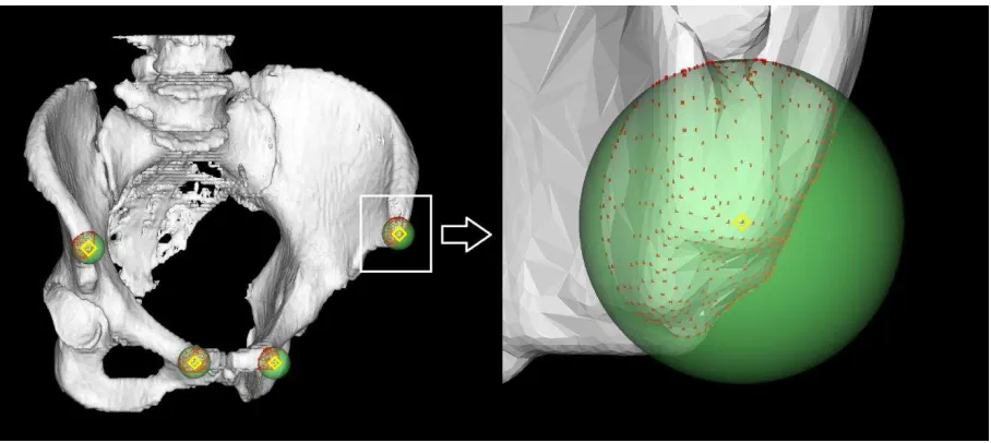
80Four initial markers are manually located on the anatomical landmarks to begin the analysis (Fig. 1). Spheres with 81
centers at each initial marker are used to clip points on the surface model. The spherical implicit function for clipping is
82
(1) 83
where is a point on the surface model Upelvis; R is the radius of the sphere, which should be large enough to
84
cover the landmark; and OP is the distance between P and the sphere center O . Thus, four clipped point sets are used 85
87
Fig. 1. Clipping landmark point sets on the pelvic surface. Four initial markers (yellow) are manually defined at positions near the landmarks.
88
Point sets (red) are clipped using a spherical implicit function (green region; see equation (1)).
89
2.1.1 Anterior pelvic plane
90
The APP can be considered as a tangent plane containing the ASISs and the pubic tubercles. The initial APP consists 91
of the initial ASIS marker bilaterally and the midpoint between the markers on the left and right pubic tubercles. At each 92
step of the iteration, points in the clipped point set are sorted by their displacement relative to the APP determined by the 93
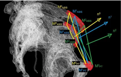
current markers. The most anterior point becomes the next marker, and the APP is recomputed (Fig. 2). The algorithm will 94
96
Fig. 2. Schematic diagram of the APP iteration. Automatically searching the most anterior point on the landmarks (red), markers are modified
97
from M0
to M2
(yellow blue green) within a few steps. The corresponding normal vector of the APP changes from n0 to n2. 98
1. Manually locate initial markers Mi0 ( i is left ASIS, right ASIS, left pubic tubercle, or right pubic tubercle).
99
2. For markers M , compute the midpoint ik k mid
M between pubic tubercles and create a plane k
APP with normal 100
vector k
n defined by bilateral MkASIS and k mid
M . 101
3. Select vertices near the markers using the spherical function in (1) (points outside of the sphere are removed). 102
Traverse every point and compute their distance to the plane k
APP ( k
n is the positive direction). 103
4. If the points with maximal distance to k
APP are not the same as markers k i
M , go to step 2; else go to step 5. 104
5. Output the last plane k
APP and normal vector k
n to be the optimal APP solution. 105
2.1.2 Midsagittal plane
106
The MSP is computed as the mirror plane associated with approximately symmetrical structures in the pelvis. An 107
initial estimate of the MSP passing through the midpoint between ASISs with a normal vector
1, 0, 0
in the world 108110
Fig. 3. MSP computation pipeline.
111
Then, the initial mirror shape is registered with the original shape using the ICP algorithm. After iterative 112
computation, the optimal registration transform is 113
(2) 114
where
T
IMis the initial mirror transform andT
ICPis the rigid ICP transform. However,T
opt is actually an affine 115transform rather than the optimal mirror transform of the pelvis. Based on the order of surface points listed in the data, 116
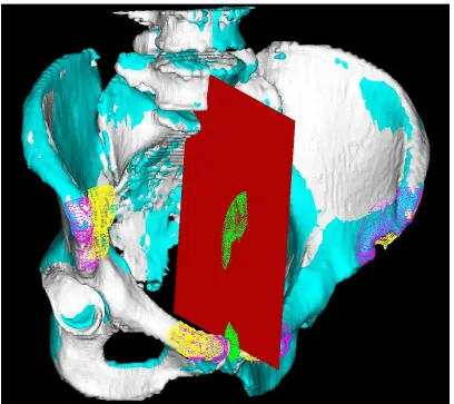
Because these points are all considered to be on the optimal mirror plane, a fitted least-squares plane (Fig. 4) should be the 118
MSP solution at the end of the computation. 119
[image:9.612.109.517.141.504.2]120
Fig. 4. MSP computation process. The initial mirrored shape (yellow) is transformed to maximally fit the original shape (white) after ICP
121
registration. The midpoints (green) between corresponding points in the original shape and registered shape (purple) are used to fit a
122
least-squares MSP (red). Visualization of the optimal mirrored pelvis (indigo) after MSP modification indicates a good result.
123
From the clinical perspective, the ASISs and pubic tubercles could provide a reliable reference because they are 124
easily accessible when the patient is in the lateral position. However, from the graphical perspective, taking the entire 125
pelvis into account would provide a benefit, such as a more accurate estimate. 126
2.1.3 The origin of the PCS and transverse plane
127
Because the APP and MSP are computed without a perpendicularity constraint, it is necessary to modify one of 128
them to guarantee perpendicularity. We recommend modifying the MSP rather than the APP because the MSP has a higher 129
clinical significance. The normal vectors associated with the MSP and the APP provide the orientation of two coordinate 130
(3) 132
where , , and are the normal vectors of the APP, MSP, and TPP, respectively. A guaranteed 133
perpendicular MSP normal is then computed from 134
(4) 135
To compute the pelvic origin OPCS, one of the markers on the APP is projected onto the MSP and then projected onto the 136
TPP. 137
2.2 Acetabular anatomy
1382.2.1 Acetabular opening circle
139
A recently published method introduced the use of a three-point circle as an initial estimate of the acetabular rim [24]. 140
However, the rim is usually not precisely circular. Our proposed method takes this into account. First, a series of nodes are 141
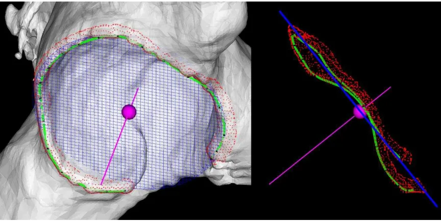
manually located along the curved osseous ridge, and a cubic interpolation is used to build a B-spline path (Fig. 5). Then, 142
surface points near the rim path are selected using a Boolean combination of spherical implicit functions. The clipping 143
function that takes the minimum value of all implicit functions is 144
Fmin
F F1, 2,...,Fn
(5) 145where Fi is a single spherical implicit function, as shown in (1), with its center at a point on the rim path and n is the 146
148
Fig. 5. Acetabular opening circle and axis determination. With about 20 nodes (black dots) manually located on the osseous ridge, a B-spline
149
path (green) is built as the rim path using cubic interpolation. Points (red) on the surface model and near the rim path are collected to fit a
150
least-squares spatial circle (blue grid). The center of rotation (purple sphere) and the normal axis of the opening plane (purple line) are
151
computed.
152
These points on the rim represent many important anatomic parameters of the acetabulum, such as orientation, shape, 153
and size. Spatial circle fitting is a convenient approach used to analyze the rim points. Here, we use a least-squares spatial 154
circle, which is actually the intersection between a sphere and a plane that are separately fitted. Finally, the anatomic 155
parameters of the acetabulum, such as those listed above (orientation, shape and size) can be easily computed from the 156
acetabular opening circle in the PCS. 157
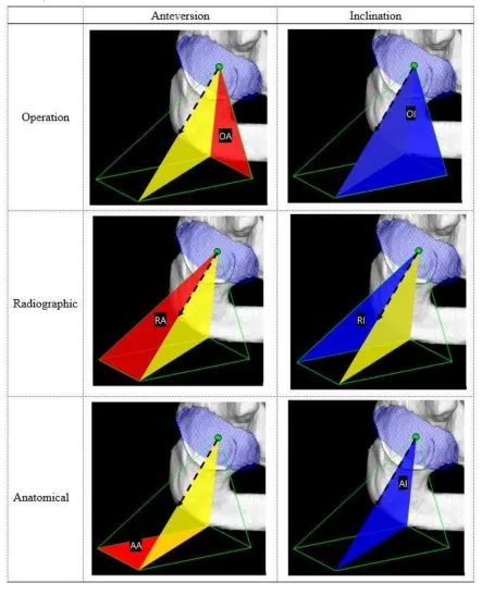
2.2.2 Acetabular orientation in PCS
158
Standard measures of anteversion and inclination of the acetabular axis have been introduced elsewhere [6]. The axis 159
vector representing the acetabular orientation calculated by the plane fitting is in the image data coordinate system and 160
the acetabular parameter calculation must be based on the standardized PCS, describing the orientation of the acetabulum 161
in 3D space. For the illustration of the PCS, please refer to Fig. 3. in [25]. 162
To determine these measures in the PCS, the acetabular axis should be transformed in advance as 163
(6) 164
vector of the acetabular axis; and I is an identity matrix. With the normalized vector , the acetabular 166
orientation parameters are computed as 167
2 2
2 2
2 2
tan
tan
tan
tan
tan
tan
OA y z
OI x y z
RA y z x
RI x z
AA y x
AI x y z
(7) 168
where OA is operative anteversion; OI is operative inclination; RA is radiographic anteversion; RI is radiographic 169
inclination; AA is anatomical anteversion; AI is anatomical inclination. (As shown in Fig 6., red represents anterversion 170
172
Fig. 6. Definition of the acetabular version
173
3.
Experiment and evaluation
174render the results of acetabular orientation. After importing the model, our proposed semi-automatic system can quickly 176
calculate the orientation. 177
For evaluation experiments, the right acetabulum was chosen. High-resolution CT data with a slice thickness of 1 mm 178
and an average in-plane (x-y) resolution of 0.977 mm of 88 normal people (mean age of 4327 years, 51 male and 37 179
female) receiving pelvic scans for reasons not related to orthopedic conditions were selected from Shanghai Nine 180
People’s Hospital institution’s database.
181
It is important to evaluate the accuracy of the APP and MSP computations. Theoretically, the APP is a unique 182
solution, and practically it can be obtained after at most four iterations. Rapid convergence required only one iteration in 183
60 cases (68.5%), two iterations in 21 cases (23.9%), three iterations in 5 cases (5.7%), and four iterations in 2 cases 184
(2.3%). The average number of iterations was 1.42±0.33, and the maximum was 4. Due to the complex 3D morphology 185
of the pelvis, evaluation of the MSP computation should also be surface-based. The point-to-surface distances between the 186
mirror pelvis and the original pelvis for every vertex of the model (Fig. 7) averaged over all 88 subjects was 1.340.49 187
mm. As illustrated in Fig. 3, the ICP shape is the optimal mirror shape. 188
[image:14.612.117.521.412.709.2]189
Fig. 7. Color-coded point-to-surface distances between the mirror pelvis and the original pelvis for every vertex.
This method performed well in the determination for all of the 88 subjects. The major error source from observers 191
was the randomness of the placement of the initial markers, especially for the two endpoints of the rim path. Different 192
observers placed the endpoints at different positions on the osseous ridge or in the notch. To evaluate the differences 193
among raters and surface models, we produced three surface models of a random patient using different threshold values in 194
segmentation, mesh smoothing, and decimation in reconstruction. Taking the parameter of the radiographic anteversion of 195
acetabulum as an example, the experiment for the patient showed that values were similar across models and raters (Table 196
[image:15.612.132.480.288.369.2]1). 197
Table 1. Radiographic anteversion of acetabulum with different raters and surface models 198
Yiping Wang Henghui Zhang Liao Wang SD
Surface Model 1 21.09° 21.52° 20.99° 0.23°
Surface Model 2 21.06° 21.04° 20.84° 0.099°
Surface Model 3 21.21° 20.69° 21.5° 0.33°
SD 0.065° 0.34° 0.28°
Henghui Zhang and Liao Wang are clinical raters, while Yiping Wang is a technical rater.
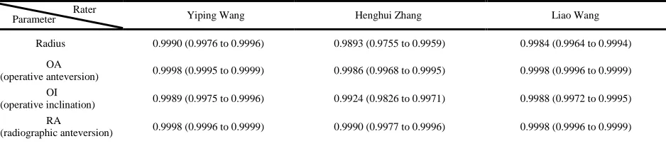
199
The intra-class correlation coefficient (ICC) evaluation is a two-way analysis of variance model that accounts for 200
random effects of both different users and subjects and it has been widely adopted to assess the reliability for a group of 201
typical users [26]. In this study, ICC scores on anteversion and inclination in the standard angular definitions (operative, 202
radiographic, and anatomic) and the radius of the acetabular rim were used to evaluate the reliability. Three trials were 203
independently performed by three raters (Yiping Wang, Henghui Zhang, and Liao Wang) on all subjects. Raters started 204
with raw DICOM (Digital Imaging and Communications in Medicine) images and performed all operations such as 205
thresholding, segmentation, reconstruction, and initial marker placement using the 3D software. Both intra- (Table 2) and 206
inter-rater (Table 3) ICC scores on these measures are high, indicating that the algorithms are very reliable and capable of 207
accomplishing repetitive measurements for mass patient data. 208
Table 2. Single measure intra-rater reliability 209
Yiping Wang Henghui Zhang Liao Wang
Radius 0.9990 (0.9976 to 0.9996) 0.9893 (0.9755 to 0.9959) 0.9984 (0.9964 to 0.9994)
OA
(operative anteversion) 0.9998 (0.9995 to 0.9999) 0.9986 (0.9968 to 0.9995) 0.9998 (0.9996 to 0.9999)
OI
(operative inclination) 0.9989 (0.9975 to 0.9996) 0.9924 (0.9826 to 0.9971) 0.9988 (0.9972 to 0.9995)
RA
(radiographic anteversion) 0.9998 (0.9996 to 0.9999) 0.9990 (0.9977 to 0.9996) 0.9998 (0.9996 to 0.9999) Rater
Parameter
[image:15.612.74.543.629.732.2]RI
(radiographic inclination) 0.9981 (0.9957 to 0.9993) 0.9893 (0.9756 to 0.9959) 0.9987 (0.9970 to 0.9995) AA
(anatomical anteversion) 0.9998 (0.9996 to 0.9999) 0.9989 (0.9976 to 0.9996) 0.9998 (0.9995 to 0.9999)
AI
(anatomical inclination) 0.9985 (0.9966 to 0.9994) 0.9910 (0.9794 to 0.9966) 0.9990 (0.9976 to 0.9996)
The values are given as the intra-rater ICC scores, with the 95% confidence interval in parentheses, for single measures in
210
terms of absolute agreement (an ICC of approximately 0.90 to 1.00 for Cronbach alpha can be considered almost perfect).
211
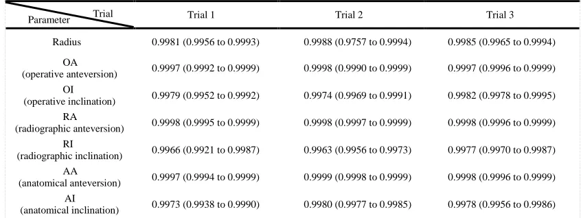
[image:16.612.93.516.229.388.2]212
Table 3. Single measure inter-rater reliability 213
Trial 1 Trial 2 Trial 3
Radius 0.9981 (0.9956 to 0.9993) 0.9988 (0.9757 to 0.9994) 0.9985 (0.9965 to 0.9994)
OA
(operative anteversion) 0.9997 (0.9992 to 0.9999) 0.9998 (0.9990 to 0.9999) 0.9997 (0.9996 to 0.9999)
OI
(operative inclination) 0.9979 (0.9952 to 0.9992) 0.9974 (0.9969 to 0.9991) 0.9982 (0.9978 to 0.9995)
RA
(radiographic anteversion) 0.9998 (0.9995 to 0.9999) 0.9998 (0.9997 to 0.9999) 0.9998 (0.9996 to 0.9999)
RI
(radiographic inclination) 0.9966 (0.9921 to 0.9987) 0.9963 (0.9956 to 0.9973) 0.9977 (0.9970 to 0.9987)
AA
(anatomical anteversion) 0.9997 (0.9994 to 0.9999) 0.9999 (0.9998 to 0.9999) 0.9998 (0.9996 to 0.9999) AI
(anatomical inclination) 0.9973 (0.9938 to 0.9990) 0.9980 (0.9977 to 0.9985) 0.9978 (0.9956 to 0.9986)
The values are given as the inter-rater ICC scores, with the 95% confidence interval in parentheses, for single measures in
214
terms of absolute agreement (an ICC of approximately 0.90 to 1.00 for Cronbach alpha can be considered almost perfect).
215
216
4.
Discussion and conclusion
217We have presented a novel surface-based approach to determine key spatial parameters of the acetabulum. A new 218
PCS consisting of the APP, MSP, and TPP was derived from a 3D pelvic surface model. Based on the PCS, critical 219
acetabular parameters can be determined semi-automatically. High efficiency was achieved for the entire algorithm 220
procedure while enabling highly reproducible measurements of acetabular spatial parameters, with almost perfect inter- 221
and intra-rater ICC scores. 222
Compared with the MSP determination using simple landmark points, the surface-based approach maximally reduces 223
manual error of acetabular angle measurements and greatly improves the reliability. The computation time depends on the 224
number of points on the surface model and the number of iterations in the ICP algorithm. In this study, we chose at most 225
50 iterations as adequate and 0.001 mm as the maximum mean distance. The number of vertices on each pelvis model was 226
about 300,000. The time consumption was less than 2 seconds after selection of the four initial points for each case using a 227
standard PC, which is comparable with the study reported by Fieten et al. [22]. 228
A better description of the acetabulum should be a spatial circle. Different investigators have taken different 229
approaches to modeling acetabular orientation. Higgins et al. [24] presented a best-fit plane for describing the acetabular 230
orientation. Jó wiak et al. [27] presented a set of section planes parallel to the acetabular opening plane to search for an
231
average trend line that joins the centers of the circles fitted by the intersection curve. We took the point set on the 232
acetabular rim as a feature extraction and found that an acetabular circle could provide a succinct description, which helps 233
to determine the center of rotation. A circle with its radius, perimeter, and normal vector can be computed by combining 234
sphere-fitting and plane-fitting algorithms. An average point-to-circle error of 3.03 millimeters was obtained in the circle 235
fitting experiments. However, the main error source is not computational, but rather the complex morphology of the native 236
acetabulum. A better description of every native acetabulum may be an equation of a best-fit curve in a cylindrical 237
coordinate system. Related work is in progress, and we believe that it is meaningful not only for pre-planning and 238
image-guidance of THA interventions, but also for patient-specific design of acetabular prostheses in the future. 239
Optimal placement of the acetabular prosthesis is critical for the success of THA. However, the target placement for 240
the prosthetic component is still unknown. The current measurement of the native acetabulum as well as the acetabular 241
component is not accurate or reliable without taking the pelvis into account. Our “Acetabulometer” establishes a reliable 242
3D PCS and measures the critical acetabular parameters based on the reported PCS. Overall, the semi-automated 243
segmentation and measurement system is sufficiently fast, accurate, and reliable to be applied to the analysis of a large 244
sample. Our approach may have the potential to determine the optimal target for the placement of the acetabular 245
component in THA. 246
247
Conflict of interests
248None declared. 249
250
Funding
251(15510722200, 16441908400), Shanghai Jiao Tong University Foundation on Medical and Technological Joint Science 253
Research (YG2016ZD01, YG2015MS26), The Royal Society International Exchanges scheme (IE140967, IE141258), and 254
the EPSRC UK Image-Guided Therapies Network+ (EP/N027078/1) and EPSRC-NIHR HTC Partnership Award 'Plus': 255
Medical Image Analysis Network (EP/N026993/1). 256
Ethical approval
257 Not required. 258References
[1] Kurtz S, Ong K, Lau E, Mowat F, Halpern M. Projections of primary and revision hip and knee arthroplasty in the United States from. Journal of Bone &
259
Joint Surgery. 2007;89:780-5.
260
[2] Beckmann J, Lüring C, Tingart M, Anders S, Grifka J, Köck FX. Cup positioning in THA: Current status and pitfalls. A systematic evaluation of the literature.
261
Archives of Orthopaedic & Trauma Surgery. 2009;129:863-72.
262
[3] Lewinnek GE, Lewis JL, Tarr R, Compere CL, Zimmerman JR. Dislocations after total hip-replacement arthroplasties. Journal of Bone & Joint Surgery
263
American Volume. 1978;60:217-20.
264
[4] Archbold HA, Mockford B, Molloy D, Mcconway J, Ogonda L, Beverland D. The transverse acetabular ligament: an aid to orientation of the acetabular
265
component during primary total hip replacement: a preliminary study of 1000 cases investigating postoperative stability. Journal of Bone & Joint Surgery British
266
Volume. 2006;88:883-6.
267
[5] Murray DW. The definition and measurement of acetabular orientation. Journal of Bone & Joint Surgery British Volume. 1993;75:228-32.
268
[6] Maruyama M, Feinberg JR, Capello WN, D'Antonio JA. Morphologic features of the acetabulum and femur: anteversion angle and implant positioning.
269
Clinical Orthopaedics & Related Research. 2001;393:52-65.
270
[7] Chu C, Bai J, Wu X, Zheng G. MASCG: Multi-Atlas Segmentation Constrained Graph method for accurate segmentation of hip CT images. Medical image
271
analysis. 2015;26:173-84.
272
[8] Yokota F, Okada T, Takao M, Sugano N, Tada Y, Tomiyama N, et al. Automated CT segmentation of diseased hip using hierarchical and conditional
273
statistical shape models. Medical Image Computing & Computer-assisted Intervention: Miccai International Conference on Medical Image Computing &
274
Computer-assisted Intervention2013. p. 190-7.
275
[9] Ellingsen LM, Chintalapani G. Robust deformable image registration using prior shape information for atlas to patient registration. Computerized Medical
276
Imaging & Graphics the Official Journal of the Computerized Medical Imaging Society. 2009;34:79-90.
277
[10] Lubovsky O, Peleg E, Joskowicz L, Liebergall M, Khoury A. Acetabular orientation variability and symmetry based on CT scans of adults. International
278
Journal of Computer Assisted Radiology & Surgery. 2010;5:449-54.
279
[11] Stem ES, O’Connor MI, Kransdorf MJ, Crook J. Computed tomography analysis of acetabular anteversion and abduction. Skeletal Radiology.
280
2006;35:385-9.
281
[12] Ghelman B, Kepler CK, Lyman S, Valle AGD. CT outperforms radiography for determination of acetabular cup version after THA. Clinical Orthopaedics &
282
Related Research. 2009;467:2362-70.
283
[13] Klaue K, Wallin A, Ganz R. CT evaluation of coverage and congruency of the hip prior to osteotomy. Clinical Orthopaedics & Related Research.
284
1988;232:15-25.
285
[14] Rittmeister M, Callitsis C. Factors influencing cup orientation in 500 consecutive total hip replacements. Clinical Orthopaedics & Related Research.
286
2006;445:192-6.
287
[15] Murtha PE, Hafez MA, Jaramaz B. Variations in acetabular anatomy with reference to total hip replacement. Bone & Joint Journal. 2008;90:308-13.
288
[16] Dandachli W, Islam SU, Tippett R, Hall-Craggs MA, Witt JD. Analysis of acetabular version in the native hip: comparison between 2D axial CT and 3D CT
289
measurements. Skeletal Radiology. 2011;40:877-83.
290
[17] Puls M, Ecker TM, Steppacher SD, Tannast M, Siebenrock KA, Kowal JH. Automated detection of the osseous acetabular rim using three-dimensional
291
models of the pelvis. Computers in Biology & Medicine. 2011;41:285-91.
292
[18] Foroughi P, Song D, Chintalapani G, Taylor RH, Fichtinger G. Localization of Pelvic Anatomical Coordinate System Using US/Atlas Registration for Total
293
Hip Replacement. Medical Image Computing & Computer-assisted Intervention: Miccai International Conference on Medical Image Computing &
294
Computer-assisted Intervention2008. p. 871-9.
295
[19] Cerveri P, Marchente M, Chemello C, Confalonieri N, Manzotti A, Baroni G. Advanced computational framework for the automatic analysis of the
296
acetabular morphology from the pelvic bone surface for hip arthroplasty applications. Annals of biomedical engineering. 2011;39:2791-806.
297
[20] Nikou C, Jaramaz B, Digioia AM, Levison TJ. Description of Anatomic Coordinate Systems and Rationale for Use in an Image-Guided Total Hip
298
Replacement System. International Conference on Medical Image Computing and Computer-Assisted Intervention2000. p. 1188-94.
299
[21] Wu G, Siegler S, Allard P, Kirtley C, Leardini A, Rosenbaum D, et al. ISB recommendation on definitions of joint coordinate system of various joints for
300
the reporting of human joint motion—part I: ankle, hip, and spine. Journal of biomechanics. 2002;35:543-8.
301
[22] Fieten L. Surface-based determination of the pelvic coordinate system. Proceedings of SPIE - The International Society for Optical Engineering.
302
2009;7261:726138---10.
303
[23] Fieten L, Eschweiler J, Fuente MDL, Gravius S, Radermacher K. Automatic extraction of the mid-sagittal plane using an ICP variant. Medical
304
Imaging2008. p. 69180L-L-11.
[24] Higgins SW, Spratley EM, Boe RA, Hayes CW, Jiranek WA, Wayne JS. A novel approach for determining three-dimensional acetabular orientation: results
306
from two hundred subjects. Journal of Bone & Joint Surgery. 2014;96:1776-84.
307
[25] Zhang H, Wang Y, Ai S, Chen X, Wang L, Dai K. Three-dimensional acetabular orientation measurement in a reliable coordinate system among one
308
hundred Chinese. Plos One. 2017;12:e0172297.
309
[26] Bonett DG. Sample size requirements for estimating intraclass correlations with desired precision. Statistics in Medicine. 2002;21:1331–5.
310
[27] Jozwiak M, Rychlik M, Musielak B, Chen BP, Idzior M, Grzegorzewski A. An accurate method of radiological assessment of acetabular volume and
311
orientation in computed tomography spatial reconstruction. BMC Musculoskelet Disord. 2015;16:42.