Digital photogrammetric mapping of canopy height in a radiata pine plantation

Digital Photogrammetric Mapping

of Canopy Height in a Radiata Pine

Plantation

Antonius Bambang Wijanarto

Submitted in fulfillment of the requirements for the degree of

Doctor of Philosophy

Centre for Spatial Information Science School of Geography and Environmental Studies

Declaration

Except as stated herein, this thesis does not contain any material which has been accepted for the award of any other degree or diploma in any university nor, to the best of my knowledge and belief, does it contain any copy or paraphrase of material previously published or written by another person, except where due reference is made in the text of this thesis.

E'O.R

NOH

OAO,

Abstract

Tree height is a crucial stand characteristic in forest inventories and has been used widely to estimate timber volume, to monitor growth rate, and as an indicator of site quality. Current tree heighting relies on field measurements, with sampling rates, which are typically less than one percent. Low sampling rates produce high variation in measured parameters and reduce statistical reliability. Digital photogrammetry provides an opportunity to automate the measurement of tree heights and to generate digital models of forest canopies. A sufficiently dense canopy model, with tree height data at nearly 100% sampling rates, has the potential to improve significantly the reliability of strategic and operational forest inventory. This study investigates the utility of digital photogrammetric techniques to map tree height within radiata pine plantations.

A digital photogrammetric workstation, the Leica Helava DPW 770, was used to generate digital canopy models of both closed canopy and thinned stands. The performance of the image-matching algorithm was assessed using scanned aerial photos of different film types and scales, including colour, black and white, colour infrared, and black and white infrared, at 1:5,000, 1:10,000, and 1:15,090 scales.

Canopy height data were obtained by subtracting a DTM from the photogrammetric data. Various filtering strategies were used to process the canopy height data including median, mean tallest tree, adaptive wavelet, adaptive Fourier filtering, and NDVI-thresholding techniques. A method for improving automatically derived tree height using a limited number of manually measured tree heights using a DPW was also developed. The reliability of the derived data was assessed by comparing it with a reference DCM produced using an analytical stereoplotter at a lOm grid, and field measurements.

Table of Contents

Abstract ... i

Table of Contents ... ii

Acknowledgments ... iv

CHAPTER 1. INTRODUCTION ...•.•... 1

1.1. The Importance of Forest Inventory ... 1

1.2. Photogrammetric Measurement of Tree Height ... .3

1.3. Research Objectives ... 4

1.4. Thesis Outline ... 5

CHAPTER 2. MEASURING FOREST INVENTORY ... _ ... 6

2.1. Introduction ... 6

2.2. Field Survey ... 8

2.3. Aerial Photographs ... 11

2.4. Radar ... 18

2.5. Airborne Laser ... 24

2.6. Optical Satellites ... 28

2.7. Airborne Line Itnagers ... 28

2.8. Airborne Videography ... 29

2.9. Summary ... 30

CHAPTER 3. IMAGE MATCHING TECHNIQUES ... 31

3 .1. Introduction ... 31

3.2. Classification of Itnage Matching Techniques ... .32

3.3. Matching Algorithms Employed by Leading DPWs ... .41

3 .4. Accuracy of DBM extraction: Comparative Studies ... .44

3.5. Measuring DEMs over a Pine Forest ... .49

3.6. Summary ... 50

CHAPTER 4. DATA ACQUISITION ...•...•...•...•..•. 51

4.1. Introduction ... 51

4.2. Study Area ... 51

4.3. Aerial Photography ... 52

4.4. Ground Control Points ... 53

4.5. Digital Terrain Model. ... 54

4.6. Reference Canopy Height Models ... 56

CHAPTER 5. METHODOLOGY··· 61

5.1. Introduction ... 61

5.2. Extraction of Canopy Models ... 61

5.3. Generation of Digital Terrain Models and Digital Canopy Models ... 64

5.4. Data Processing and Filtering ... 66

5.5. Statistical Analyses ... 79

CHAPTER 6. COMPARISON BElWEEN DIGITAL AND ANALYTICAL PHOTOGRAMMETRIC DATA ...•... 81

6.1. Introduction ... 81

6.2. Analysis: the Closed Canopy Stand ... 81

6.3. Analysis: the Thinned Stand ... 99

CHAPTER 7. IMPROVING AUTOMATICALLY DERIVED DIGITAL PHOTOGRAMMETRIC

DATA ... 127

7 .1. futroduction ... 127

7.2. Methodology ... 127

7.3. Analysis: the Closed Canopy Stand ... 128

7.4. Analysis: the Thinned Stand ... 136

7.5. Summary ... 142

CHAPTER 8. SUMMARY AND CONCLUSION ... 143

8.1. Review of Research Objectives and Methodology ... 143

8.2. Summary of Results ... 144

8.3. Conclusion and Recommendation for Future Work ... 145 REFERENCES ... 14 7

APPENDICES:

Graphical User futerf ace List of Figures

List of Tables ENCLOSURE:

Acknowledgments

I would like to extend my special thanks to the following people for their contribution to this thesis.

The research was completed under the supervision of Dr. Jon Osborn, who patiently kept me on track, and facilitated my interaction with many people and organisations who directly or indirectly have supported the project.

The digital photogrammetric workstation, the Leica-Helava DPW 770, was made available by the Hydro Electric Commission (HBC) of Tasmania, Survey and GIS Division. My thanks to Mr. Keith Stove and Mr. Graham Humphries.

Access to the study area and aerial photography was provided by Fletcher Challenge Paper Australia through Mr. Tim Osborn, Mr. Andrew Dickinson, and Mr. John Webb. These people provided a great assistance, particularly in the early stages of the research.

The GPS fieldwork was completed with assistance from Nguyen Ngoc Lau, Murray Webster, Mark Morffew, Anthony Mewengkang, and Bambang Rudito. Mark Morffew generated the colour infrared orthoimage for the NDVI-thresholding described in Chapters 5 and 6, and assisted with the GPS processing.

Finally, this research was made possible through the financial support of the Tasmanian Forest Research Council and an Australian Government Overseas Postgraduate Research Scholarship.

Chapter 1. Introduction

1.1. The Importance of Forest Inventory

Forest management is concerned with ensuring a sustainable supply of timber and other forest products while maintaining sound ecological practices.

Economically viable and ecologically sound forest management can only be achieved by careful planning. The steps involved in the management of a forest usually include [Susilawati and Weir 1990]:

• forest inventory, in which information is gathered about the environment to identify where decisions and action are needed;

• planning, which permits the analysis of alternative courses of action when models are developed;

• policy-making, during which a particular course of action is selected; • operation, in which the chosen action is implemented; and

• monitoring, in which the results of the operation are reviewed.

Extensive data collection and monitoring are required to evaluate the rate and course of early plant succession, and to prescribe the necessary vegetation management treatment to fulfil the objectives of forest management. New technology such as geographic information systems can enhance decision-making, but require comprehensive and high-quality data as inputs. Therefore, data collection methods must be capable of delivering objective, quantitative, multi-dimensional, multi-scale, spatially accurate, and cost-effective data for forest management decision making and monitoring [Pitt et al. 1997].

involve very time consuming and expensive field measurements of a large number of sample plots. Surveys range from simple visual observations made from an aircraft, road vehicle, or by foot, to installation of field plots to measure variables such as vegetation height, cover, and health [Congalton and Biging 1992, Gillis and Leckie 1996].

Recognition of the importance of efficient forest inventory methods has led to extensive research and the development of various different methods for forest classification and forest size measurement. These include the applications of photogrammetry, remote sensing, geographic information systems, and other

computer-aided analysis and mapping techniques.

1.1.1. Forest Parameters and Stand Variables

Forest inventories are generally defined in terms of their function, which is to determine the extent, scale, quantity, quality and the location of both forest and non-forest parameters (Table 1.1) [e.g. Biging et al. 1991, Congalton and Biging

1992, Long 1994].

Stand (forest) tvPes Stand boundaries

Species composition,

height classes, age classes,

Stand structure density (canopy closures and stocking), variables diameter (basal area),

Forest timber defect,

volume,

leaf area index (LAI) and other stand variables Location

Conditions,

Status Thinned

Unthinned alive/cut Farmland,

Non-forest Water,

rocks, roads and tracks etc.

Table 1.1. Components of a forest inventory [adapted from Congalton and Biging 1992, Long 1994].

plantation, for example, age and type of plantation (often homogeneous), and terrain characteristics. Other parameters such as diameter at breast height (DBH) and tree height must however be measured. Generally, forest managers collect these parameters using statistical sampling methods and rely heavily on measurements of individual trees within sample plots.

1.1.2. The Need to Measure Tree Height

Tree heights are a crucial stand characteristic in forest inventory. Tree height:

• contributes to estimated timber volume;

• · is used to monitor growth rate; and

• is used as an indicator of site quality.

Tree heights are often represented using the parameters stand mean height and stand mean dominant height (MDH) [e.g. Carron 1968, Candy 1989a and 1989b]. Stand mean height is normally not the average of individual tree heights, but an approximation to it, associated with the arithmetic stand mean basal area. Fletcher Challenge Paper Australia (FCP A), who manage the plantation used in this research, defines mean dominant height as the mean height of the sixty trees with the largest diameter at breast height (DBH) per hectare.

The major objective of forest inventory is to estimate timber yield of harvesting events over time. Individual tree volume is a function of diameter at breast height (DBH), tree height and age [Candy 1989a]. Total standing timber volume for stands is a function of mean dominant height and stand basal area [Candy 1989b].

1.2. Photogrammetric Measurement of Tree Height

Tree height is a parameter that has the potential to be measured and exploited using remote sensing techniques including radar [e.g. Hagberg et al. 1995, Hyyppa

and Hallikainen 1996], airborne laser [e.g. Aldred and Bonnor 1985, Nelson et al.

1988, Jacobs et al. 1993, Nilsson 1996, Naesset 1997a and 1997b, Means et al. 1999], and aerial photography.

stereoplotters [e.g. Johnson 1958, Kippen and Sayn-Wittgenstein 1964, Aldred and Kippen 1967, Sayn-Wittgenstein and Aldred 1967, Avery and Canning 1973, Titus and Morgan 1985, Nielsen 1997, Reutebuch and Ahmed 1997], and manually using a digital photogrammetric workstation [e.g. Gagnon et al. 1993, Kovats 1997].

More detailed descriptions are included in Section 2.4.2.

The shift from analytical to digital photogrammetry offers an opportunity to automate the measurement of tree heights. Digital photogrammetric workstations include modules to generate digital elevation models (DEMs) automatically by

image matching techniques in stereo pairs of scanned aerial photographs. Over forested terrain the DEM will include tree height data. Automation has the potential to provide tree height data at nearly 100% sampling rates, with consequent potential to improve the reliability of timber volume estimates.

The use of digital photogrammetry for automatic terrain extraction has been an important innovation in topographic mapping and related applications. To date, however, very few organisations have attempted to use this advanced technology to measure forest parameters automatically, relying instead on conventional methods

of field inventory and film-based aerial photo-interpretation. This suggests a need for further study to determine the potential of digital photogrammetry to contribute to forest inventory, in particular tree height.

1.3. Research Objectives

The objectives of this study were to determine whether high resolution scanned aerial photography can be used to estimate canopy height in a Radiata pine

plantation, and to develop methods to represent the extracted data in a form that can contribute to forest inventory and management. Specific objectives were as follows:

(1) to test the application of the image matching algorithms in a digital photogrammetric workstation to estimate canopy height over various canopy types, using different scales of aerial photography and different types of film; (2) to determine the most suitable scale and film type to measure canopy height; (3) to develop, test and compare various data filtering methods to extract data

(4) to compare data derived from a DPW with tree heights measured using an analytical stereoplotter, and to quantify the accuracy of the automatic methods; (5) to develop a method for ground truthing or improving automatically derived

digital photogrammetric tree heights using a small number of manually measured photogrammetric tree heights.

1.4. Thesis Outline

This thesis is divided into eight chapters. In this chapter the importance of

forest inventory, the need to measure tree height and the objectives of the research have been introduced.

Chapters 2 and 3 provide the necessary background information for photogrammetrists and foresters. Chapter 2 is a review of relevant background information concerning forest inventory methods and Chapter 3 is a review of image matching methods employed by digital photogrammetric workstations.

Chapter 4 presents the methods and procedures used to collect field data, including tree heights, DTM data, and ground control for photogrammetric measurement. Chapter 4 also describes the acquisition of aerial photography, and the generation of a tree height model from aerial photographs using an analytical stereoplotter.

In Chapter 5, methods of measurmg tree height usmg the digital photogrammetric workstation and methods of processing the data into useful and

meaningful information are presented. The DTM extraction strategies and image processing filtering strategies are described.

Chapter 6 presents an analysis of the different tree heighting methods for both the closed canopy stands and thinned stands. In this chapter, data derived from a DPW are compared with data derived from an analytical stereoplotter. The analysis includes visual inspections and comparisons of statistical results, distributions and image profiles.

Chapter 7 presents methods for improving the automatically derived digital photogrammetric data using manually measured photogrammetric data.

Chapter 2. Measuring Forest Inventory

2.1. Introduction

Remote sensing techniques have been used with varying degrees of success in

forest inventory to measure forest parameters. Remote sensing techniques can offer high repeatability, multi-dimensional, multi-spectral, multi-resolution and GIS compatible data. Field measurement remains, however, the principal mean of data acquisition for forest inventory. Most studies have focused on coniferous forests, such as pine plantations, which tend to be more uniform and more distinguishable from other vegetation types.

There is a range of remote sensing systems capable of providing data useful to forest inventory. These include aerial photography, airborne video, line imagers, airborne laser, airborne radar, Landsat TM, Landsat MSS, SPOT and Radarsat. The characteristics of these sensors are summarised in Table 2.1.

Sensor Pixel size Image swath Stereo Spectral Characteristics Image Geometric Weather Potential uses

viewine: form correction Reauirement

Aerial photos Easy Visible and near IR Film or Easy Clear to light Mapping

scanned cloud cover Stratification

Depends on flying height, lens' focal digital Sampling

Digital camera Easy Visible and near, mid and Digital Easy Clear to light Mapping

length, and sensor format. Typically,

thermal IR (3 to 8 bands) cloud cover Stratification resolution of aerial photo > digital

Sampling Airborne Video camera > airborne video Moderate Visible and near, mid and Analog or Moderate Clear to light Stratification

thermal IR (3 to 8 bands) digital cloud cover Sampling

CASI No. of bands and flying _{150m to 5km Difficult} Visible to near IR (1 to 19 Digital Difficult Clear to light Stratification

height influence the spatial _{bands) cloud cover Sampling}

resolution, e.g. 30cm can be achieved from I band, 60cm from 5 bands and Im from 10

bands at same flying height

LandsatMSS 79mand 82m 185km No Visible+ near IR (4 bands) Digital Easy Cloud-free Mapping Stratification

LandsatTM 30m 185km No Visible, near and mid IR (6 Digital Easy Cloud-free Mapping

bands) + thermal IR @ 120m Stratification

SPOT 10mor20m 65km Difficult Panchromatic visible, near IR Digital Easy Cloud-free Mapping

(3 bands) Stratification

Airborne radar >lm >4km Difficult Microwave Digital Difficult None Mapping

Stratification Sampling

Radarsat >lOm 50-500km Easy Microwave Digital Moderate None Mapping

Sampling

Laser, LIDAR 10-50cm Point NIA Generally near IR Digital Moderate No rain Sampling

Table 2.1: Typical sensor characteristics [adapted from Pitt et al. 1997].

2.2. Field Survey

2.2.1. Introduction

Field survey is currently still the principal means of collecting forest parameters.

In a forest inventory that involves remotely sensed data, it is necessary to check the data with the field measurements. The field-measured data (ground truth data) can be used to overcome any confusion in forest measurement or classification, and to improve forest inventory results. The following are two approaches to collecting ground data [e.g. Congalton and Biging 1992, Gillis and Leckie 1996]:

(i) Visual census

In this approach, a field crew will visually carry out a census of dominant species, size class of dominant species, crown closure of dominant size class, and crown closure of all tree species combined. This type of survey can be made from an aircraft, road vehicle, or by foot.

(ii) Plot measurement

A plot is a permanent or temporary-sampling unit established in forests to collect forest parameters. The size and shape of plots may vary with forest conditions. The shapes may be regular, for example, rectangular, square, circular, narrow-width rectangular; or they may be irregular, for example, basal-area sweeps. The relative efficiency of different sizes and shapes is influenced by the purpose of the inventory, and can be compared by estimating the respective sampling errors [Gambill et al. 1985]. As a guiding principle, the size of a plot must be related to the elements of the population. A typical plot size for a coniferous plantation forest is between 0.005 and 0.01 hectares [e.g. Gambill et al.

1985].

In plot measurement, there are two types of variables: estimated and measured. The estimated variables include:

•

•

•

•

• height,

• leaf area index (LAI), • crown closure, and • crown size.

The most difficult variables to measure are usually crown closure and tree height, which require considerable experience to obtain adequate precision [Congalton and Biging 1992].

2.2.2. Tree Height Measurement

There are three representative methods of measuring tree height in the field: height-matching method, distance-measure method, and angle-measure method [e.g. Koming and Thomsen 1994].

(i) Height-matching method

This method involves one observer at a point where the entire tree can be seen, who matches the top and the base of the "tree to the ends of a hand-held object of length l (Figure 2.1). From the base of the object, a portion of length p is marked. A second person at the base of the tree lifts a rod (height

=

h

h=

f

xl.

p

d

(ii) Distance-measured method

In this method, one horizontal distance (d) and two angles (A and C) are measured (Figure 2.1). The horizontal distance (d) is measured from the tree to an observation point. The angles are measured using a clinometer. These are the angle between the horizontal plane and the treetop (A) and the angle between the horizontal plane and the tree base (C). The height his calculated as

h =d(tanA+tanC).

(iii) Angle-measured method

In this method, three angles A, B and Care measured (Figure 2.1). B is the angle to the top of a pole of length/, placed at the base of the tree. The tree height h can be calculated from

h- (tanA-tanC)

- (tanB-tanC)"

The accuracy of tree height measurements using the methods described depends on several factors including the accuracy of the vertical angle and/or distance measurements, and the visibility of the tree. Vertical angles are usually measured using a clinometer, and distances are measured using a tape or an electronic device. Measurement of distance using a tape is not as efficient as using an electronic device. However, measurement using an electronic device requires a good visibility or clearance to the tree being measured. Further, angle measurements require good visibility to the top and the bottom of a tree, which can be difficult

especially in dense forests.

2.3. Aerial Photographs

2.3.1. Introduction

Aerial photography is regarded as a reliable method to measure some forest parameters and has played a key role in forest mapping and inventory systems. It is the most frequently utilised remote sensing tool for forest assessment [Gillis and Leckie 1996]. Aerial camera performance has been improved by computer designed lenses, forward motion compensatio!l, angular motion stabilisation, and integrated geopositioning and exposure control systems [Fent et al. 1995, Light

1996]. Aerial films have also been improved to address issues such as film speed, spectral sensitivity, resolution, colour rendition, and processing [Fent et al. 1995].

Factors that influence the reliability of aerial photography are described in the

following Sections.

2.3.2. Considerations in the Use of Aerial Photographs

The most important consideration when preparing specifications for aerial photography is the photographic scale. Photographic scale is a critical determinant of photo-interpretability. Therefore, the choice of scale can maximise the utility of photographs for particular projects.

A wide range of photographic scales has been used for forest inventory. Usually, the smaller scales have been used for mapping forest types and estimating stand volumes, whereas large-scale photographs have been used for tree volume estimation and regeneration assessment. Table 2.2 summarises several information thresholds according to the photographic scale or image resolution. Other factors include:

( 1) Camera geometry: The geometry of a camera system affects the visual penetration of forest canopies. For a given camera format, longer focal lengths provide greater penetration than shorter focal lengths for photographs at the same scale, but result in weaker vertical geometry and less ground coverage for a given flying height.

1

2 3

4

5 6

extensively in API for forest inventory and they are generally superior to black and white photographs for forest mensuration from aerial photographs. Black and white film may offer some advantages including, for example, high spatial resolution and smaller file size when scanned. Infrared films (colour or black and white) are also used in forest inventory. The advantages of using IR film include the ability to interpret and measure energy spectra which are not visible to the human eye, and the ability to measure forest parameters which depend on spectral sensitivity in the near infrared, for example, tree health and species [e.g. Elvidge 1990].

Photo-scale Forest characteristics Remarks

<1:30,000 Forest/ non-forest, evergreen Tone, colour contrast, I deciduous /mixed, some size textural contrast, site, stand classes, occasional forest types, height, crown cover, crown stand size classes, stand size (qualitative)

physiognomy, some forest types

1:30,000 to 1:25,000 As 1, more details As 1, API easier 1:20,000 to 1:10,000 As 1, forest types, stand volumes, As 1, but quantitative,

tree volumes, some tree species, and photogrammetric understorey data measurement (E.g. Tree

height)

1:10,000 to 1:8,000 As 3, stand composition by tree As 3, colour/tone contrast

species within tree crowns

1:5,000 to 1:4,000 As 4, individual tree species As 4, branching habit >1:2,000 As 5, tree species identification, As 5, crown details

more reliable tree volumes, improve shrub characteristics

Table 2.2: Forest information thresholds over a range of aerial photographic scales [adapted from Howard 1990: 270].

(3) Sun angle and illumination: Appropriate sun angle and illumination conditions can provide aerial photographs with reduced shadow: shadowless photography results in significant advantages when understorey and ground conditions are to be interpreted [e.g. Bradshaw 1974, Bradshaw and Chandler 1978], and when tree heights are to be measured [e.g. Lyons 1967, Spencer 1979].

superior to prints [Welch 1968] with film diapositives widely used in photogrammetric applications. For digital processing, the films are scanned. The choice of scanning resolution affects the interpretability of digital images and the file size.

Photogrammetric scanners must provide high spatial resolution and high radiometric and geometric accuracy. The typical specifications of ten photogrammetric scanners are summarised in Table 2.3.

Brand Model Geometric Radiometric Price

accuracy (um) accuracy (DN) (US$)

LHSystem DSW300 2 1-2 145,000

Zeiss SCAi 2 ±1.5 138,000

XL Vision, ISM Ortho Vision, XL-10 <3 - 95,000

Vexcel Imaging VX4000 ±2 ±2 60,000

Wehrli and Assoc. Inc RM-2 Rastermaster -

-

Zeiss/ Intergraph PhotoScan 1 <2 ±2 147,000

Int'l Svstemap DiSC 5 - 75,000

Lenzar Lenzpro 2000 <3 or 0.1 pixel ±2.5 165,000 Multimedia

DBA System Inc. DFS 1 - 350,000

GeoSystem Delta-Scan 3 - 25,000

Table 2.3: Photogrammetric scanners (status January 1998) [Adapted from Baltsavias 1998].

2.3.3. Tree Height from Aerial Photographs

2.3.3.1. Photo Measurement

Photo interpretation and measurement may be grouped into two categories: direct and indirect measurements. Direct measurements are taken directly from the photograph, and these include stand height, visible crown diameter, and degree of stocking (individual crown count and percent crown cover). The only errors considered in direct measurements are sampling errors and related measurement errors. Indirect measurement, such as stem diameter at breast height,

form

timber. Conventionally, there are three methods of height measurement: (i) measurement of displacement using a single photograph,

(ii) measurement of shadow length, and

(iii) measurement of parallax differences on stereophotography.

The main difficulty is finding the ground in a dense forest. The measurement of tree heights using stereophotography is commonly still based on conventional methods in which the operator places a floating mark onto the ground as close as possible to the base of a tree and then places the floating mark on top of the tree. In

a dense forest, the photo interpreter must look for a hole in the canopy and then

decide whether the surface seen at the bottom is the ground or vegetation with a significant height. Measurement is usually easier when the aerial photographs are taken after the forest has been thinned or cleared.

2.3.3.2. Tree Height from Large-scale Photography

Large-scale photographs have been used to measure tree height using simple parallax heighting methods [e.g. Andrews 1936, Johnson 1958], analogue stereoplotters [e.g. Kippen and Sayn-Wittgenstein 1964, Aldred and Kippen 1967, Sayn-Wittgenstein and Aldred 1967, Avery and Canning 1973], analytical stereoplotters [e.g. Titus and Morgan 1985, Nielsen 1997, Reutebuch and Ahmed 1997], and digital photogrammetric systems [e.g. Gagnon et al. 1993, Kovats 1997].

Various large-scale camera systems have been designed such that the photoscale

can be calculated without reference to ground control so that reliable measurements can be obtained at low cost. Two such methods are:

(i) sequential photography with known flying height, and (ii) fixed-based photography.

Sequential photography involves a single camera. Photographic scales for the sequential photography method are calculated from the flying height determined with a precise altimeter. Fixed-based photography involves simultaneous exposure of two cameras, mounted on supports at a fixed and known separation and orientation. Photographic scales are calculated from the known separation and orientation of the stereo camera.

relationship between scanning resolution and tree height accuracy over a coniferous plantation forest (black spruce and white pine) has been investigated by Gagnon et al. (1993). Aerial photography was acquired at 1:1,100 scale with lOOm flying height, a base/height ratio of 0.1, and a stereo overlap of 80%. The camera used was a 70mm format Hasselblad with lOOmm focal length lens. The photographs were scanned at three resolutions: 300, 450 and 600 dots per inch (equivalent to approximately 80, 55 and 40µm, respectively). Tree heights were measured manually using a floating mark in the stereo display. A point on the ground, which also appeared on the photograph, was used as the datum. Twenty-four trees (12 black spruce and 12 white pine) were measured and the results were compared against ground truth data. Standard deviations of ±0.48m, ±0.32m and ±0.24m were achieved for scanning resolutions of 300, 450 and 600 dpi, respectively.

The investigation conducted by Gagnon et al. (1993) demonstrates that scanning resolution affected the accuracy of tree height measurement, at least for manual measurement using a floating mark on the screen. The results also indicate that precision comparable to field measurements can be achieved using scanned, large-scale photography. In practice, the method could be used to replace field-measured tree height for small areas, such as for plot measurement. The method is relatively inexpensive since it employs small format photography and a low precision scanner. A disadvantage of the method is the problem of finding a visible ground surface.

A similar method was developed using a helicopter mounted with a pair of 70mm format cameras and lOOmm focal length lenses, and using a fixed wing aircraft with 230mm format camera and 152mm focal length lens [Kovats 1997]. The photographs were acquired at several photoscales (1:800, 1:1,000 and 1:1,200) over a coniferous plantation forest of 3000 sample trees. Permanent ground control was placed across the study area prior to photography. The photogrammetric results were compared against ground truth data. Standard deviations of the differences from the ground truth data were ±0.34m at 1:800 scale for the helicopter photography and ±0.80m at 1:1,200 scale for the fixed wing photography.

demonstrates that large-scale photography can be used to measure tree heights with precision comparable to field measurement techniques. However, the method relies on many permanent targets over a large area, which must remain visible even when the trees have grown taller. On-board integrated GPS-inertial navigation systems at reasonable costs are not sufficiently accurate to replace ground control at these photoscales.

Other large-scale applications have been the use of small-format aerial

photography to acquire detailed forest data [e.g. Nielsen 1997] and to monitor stand development using a twin camera helicopter boom [e.g. Reutebuch and Ahmed 1997].

2.3.3.3. Tree Height from Medium and Small-scale Photography

Tree heights have been measured using a pocket stereoscope and a parallax bar in the study by Allison (1956). Photographs were acquired at 1:10,000 and 1:20,000 scales from a combination of flying heights and 3.25-inch and 8-inch

lenses. The photo-measured tree heights were compared against ground truth data. Under ideal conditions, tree heights were measured to within ±l .5m and ±3m from the ground truth data on 1:10,000 and 1:20,000 scale photography, respectively.

A similar technique was investigated by Johnson (1958) using both a parallax wedge and a parallax bar on 1 :5,000, 1: 10,000, 1: 15,000 and 1 :20,000 photographs. The method employed three different operators and various combinations of instruments, photographic scales and operators. In contrast to the finding of

Allison (1956), Johnson found that errors in measured tree height were not associated with photographic scales, at least in the range from 1:5,000 to 1:20,000, but more likely associated with tree characteristics such as crown shape and tree size, and instrument operator skills.

No published research has been found that indicates the accuracy of tree height measurement from medium to small-scale photographs using analogue or analytical stereoplotters.

2.3.3.4. Mapping Tree Height Using a DPW - Previous Research

Carson et al. (1996) used a digital photogrammetric workstation to generate digital canopy models of forested areas in New Zealand using aerial photographs at four epochs: 1971, 1981, 1988 and 1994. The photographs were acquired at a scale of 1:25,000. The 1994 photography was in colour, whereas the previous photography was in BW. The images were scanned at 12.5µm to give a pixel size of approximately 0.3 lm. The areas consisted of mainly Radiata pine plantations, which were planted in 1973 and 1980. The different-epoch photographs provided different types of canopy closures (Table 2.4).

Area Acres 1971 1981 1988 1994

1 40.0 Bare Good crown closure Thinned Thinned again (planted in 1973)

2 10.6 Bare Planted in 1980 Good crown closure Heavily thinned 3 17.0 Bare Good crown closure Good crown closure Good crown closure

(planted 1973) but thinned

Table 2.4: Test areas [Carson et al. 1996].

A Leica-Helava DPW 770 was used to generate a canopy model of the forested areas. The DEMs were produced at 2m spacing using a variety of strategies. The strategies applied in this study were not described. The 1971 photography was used to generate a DTM of each area. The canopy height models were generated by subtracting the DTM of the 1971 photography from the canopy models of the 1981, 1988 and 1994 photography. The results are summarised in Table 2.5.

Area Period Mean (m) Standard Deviation (m)

1971-1981 12.37 2.22

1 1971-1988 10.80 10.10

1971-1994 18.45 9.70

1971-1981 0.17 0.95

2 1971-1988 11.29 2.10

1981-1994 2.39 6.37

1971-1981 12.30 2.42

3 1971-1988 20.90 3.04

1971-1994 9.49 15.85

As indicated in Table 2.5, the results were encouraging in areas of good canopy closure, but less encouraging in areas where the plantations had been thinned. In

the thinned areas, the errors, as reported by Carson et al. (1996), were associated with the more irregular canopy structures produced from the thinning, in which more of the ground surfaces and long dark shadows of the trees were visible.

The 2m grid spacing used by Carson et al. (1996) was sufficient to create canopy models but not to model individual trees, especially for a coniferous shape. Further, with a 2m grid spacing the probability of any grid point falling on or very close to the top of a tree is reduced. This suggests a need to investigate a higher s~pling rate or a denser grid spacing particularly over thinned canopies.

2.4. Radar

2.4.1. Introduction

Radar is an active remote sensing device that has developed rapidly for topographic mapping. Radar data can be collected from an aircraft (airborne radar systems) or from a satellite (spaceborne radar systems). Radar is able to penetrate cloud, operate in all weather conditions, and cover large areas in a single flight [e.g. Elhassan and Ali 1995].

A radar instrument emits microwave pulses to a surface via a transmitter. These pulses are reflected by the surface and a small part of this reflection can be detected by the radar antenna. Radiation reflected in the direction of the radar sensors is called backscatter. The amplitude and phase of the signal received by the antenna depend on the reflection at the surface. Variations in the intensity of backscatter, the time taken to return to the radar sensor, and the phase information, provide the fundamental data for Radar remote sensing [van Halsema and Hansen 1996].

2.4.1.1. Radar Wavelength and Polarisation

Radar is classified by its wavelength and polarisation. Radar wavelengths are classified into bands (Table 2.6).

1987]. Polarisation in radar is also divided into two types: like polarisation and cross polarisation. Radar is said to be like polarised (or co-polarised) when the send and receive polarisation have the same orientation, and cross-polarised when the two polarisations are opposite. The send and receive polarisation are usually denoted as two letters: H for horizontal and V for vertical; for example, VH indicates the vertical send and horizontal receive.

Band Wavelength (cm) Frequency (MHz)

K, 0.75-1.10 40,000-26,500

K 1.10-1.67 26,500-18,000

K,, 1.67-2.40 18,000-12,500

x

c

s

L 15-30 2,000-1,000

p _{30-100 1,000-300}

Table 2.6: Radar bands, wavelengths and frequencies [Adapted from Lillesand and Kiefer 1994: 668].

2.4.1.2. Imaging and Non-Imaging Radar

Radar may also be classified into imaging and non-imaging radar. Non-imaging radar systems are generally used for non-topographic mapping. The systems utilise low look angles and use Doppler shift to measure distance. hnaging radar systems use higher look angle (usually >20°). The systems are also referred to as side looking radar (SLR) or side looking airborne radar (SLAR). The backscatter

signals detected by the radar sensor are recorded as pixel gray level values. One advantage of imaging radar is that the images produced can be viewed stereoscopically.

Synthetic aperture radar (SAR) is an imaging radar device developed to overcome the technical difficulties of constructing a very long antenna. In radar systems, longer antennas provide higher ground resolution and satellite radar would require a very long antenna in order to achieved desirable ground resolution. Modem spacebome SAR now has multi-wavelength polarimetry (HH, HV, VH, and VV polarisation).

2.4.1.3. Radar Interferometry

different SAR images of the same terrain, taken from slightly different positions or at different times. The changes of the path length can be measured and related to either surface topography or topographic deformation. A specially designed interferometry SAR would usually consist of two antennas. One antenna both transmits and receives the radar signal, while the second receives only. A spacebome SAR has only one antenna; therefore, the repeatability of the satellite's orbit must be used. This method is called 'repeat pass interferometry' or 'across track interferometry' [Hagberg et al. 1995, van Halsema and Hanssen 1996].

The technique has some similarities to stereoscopic photogrammetry [van

Halsema and Hanssen 1996], however there are two significant differences. In photogrammetry, the two overlapping images or photos have a baseline in the order of 60% of the height of the sensor (somewhat greater in the case of a superwide angle lens and less in the case of a normal angle lens), but for the SAR interferometry technique the baseline should be small since the scattering pixel can no longer be compared if the sensors are too far apart. The other significant difference is the definition of vertical resolution. The vertical resolution in photogrammetric techniques is usually a function of base to height ratio, whereas the vertical resolution in the interferometry technique is a function of wavelength.

Interferometric SAR (INSAR) is a promising technique for the production of detailed and accurate three-dimensional relief data of the Earth's surface, and detection of cm-scale movement of land surface features [Coulson 1996]. The

technique has been used to measure mm-scale ground motion in agricultural fields using SEASAT data [e.g. Gabriel et al. 1989], and cm-scale tom-scale co-seismic displacement [e.g. Massonnet et al. 1993, Massonnet et al. 1995].

2.4.2. Applications of Radar in Forestry

There have been a number of attempts to use radar for forest inventory, using single or repeat pass interferometry and single or multi-frequency radar data. For example, forest biomass, tree geometry, and canopies have been measured using P band [e.g. Rignot et al. 1995], L band [e.g. Reich and Russin 1993], and multi-frequency (bands P, Land C) [e.g. Ranson and Sun 1994, Ferrazzoli and Guerriero

attempts to measure tree height using multi-frequency radar [e.g. Hagberg et al. 1995, Dobson et al. 1995, Hyyppa and Hallikainen 1996].

There are some important characteristics of radar, which may be useful when applied to forestry:

• Radar response is strongly influenced by the surface roughness characteristics of the object being mapped, incidence angle and the dielectric propertie~ of the object [e.g. Bryan 1981, Brown 1987, Weishampel et al. 1994, Wilson 1996].

• Radar backscatter is a function of both the vertical and horizontal distribution of vegetation. The return signal strength is determined by tree height, trunk diameter, branching pattern and canopy characteristics as well as the

distribution and size of plants within the resolving element of the radar system [e.g. Milne et al. 1996].

• The amount of penetration into the vegetation is a function of the radar frequency, as well as vegetation density and moisture content [e.g. van Zyl 1996].

2.4.3. Tree Height from Radar

There are two techniques that can be used to measure tree height for inventory using a radar system. These are interferometric and polarimetric techniques. Digital elevation models (DEM's) over forested terrain can be produced from repeat pass SAR interferometry. Tree heights can be measured in combination with

another DBM or by combining interferograms at two different frequencies, for example using C and P bands (P band penetrates the canopy more than C band). The like polarisation gives a clear radar return both from the treetops and the ground. The ground reflections are partly due to penetration and partly due to gaps in the canopy.

Hagberg et al. (1995) used repeat pass interferometric techniques with ERS-1 SAR at C band to measure tree heights of fir canopies over relatively flat terrain. The ERS-1 SAR has a typical image coverage of 80 x 80 km and a pixel spacing of

weather conditions such as temperature and wind. The results from radar measurements were compared to tree heights obtained with conventional field measurements. Hagberg et al. found that over a dense forest with an average height of 15.6m measured in the field, the interferometric method measured the forest at an average height of 14.9±1.6m and that over more sparse forest with an average height of 9.9m measured in the field, the interferometric method measured the forest at an average height of 4.9±1.6m. Both results were obtained from baselines longer than lOOm. In terms of weather conditions, the interferograms were found to be sensitive to air temperature, but not to wind condition. This was because of the stiffness of the fir canopy. Other types of forests may have different responses to wind.

Dobson et al. (1995) used polarimetric data derived from SIR-C/X-SAR data at L and C bands to estimate tree height in mixed forests including some types of coniferous trees. The fully polarimetric SIR-C data at L and C bands (VV polarised X-SAR data at X band) were processed. The pixel resolutions were 24.6mx26.9m for the Land C bands, and 25.5mx22.5m for the X band. Ground control points were used to co-register X band to the L and C bands of the SIR-C data, with an accuracy of ±25m.

Group Local Species Polarisation No.of Correlation RMSE

Name components Cases (R2)

Long needle Upland conifers L,vv 40 0.78

Short needle Lowland conifers L,vv-C,vv 4 0.63 Small branches, Lowland conifers L,vv-C,hv 4 0.95

small needle

Small branches, Upland conifer L,vv/L,hv 20 0.78 medium needle (Jack pine)

Large branches, Upland conifer L,vv 19 0.89

long needle (Red pine)

Table 2.7: Accuracy of tree heighting using polarimetric SIR-C data

over coniferous forests [adapted from Dobson et al. 1995].

(m) 4.14 0.62 4.21

1.47

3.45

conventional field measurements (Table 2.7). The recorded heights in the area ranged from 0-23m.

Hyyppa and Hallikainen (1996) used an airborne profiling radar system to measure tree height of pine and spruce dominated forests of variable density. In

sparse stands, for example, there were less than 12 trees per plot (20m x 20m). The radar stand profiles were collected using a helicopter-borne ranging scatterometer, HUTSCAT (Helsinki University of Technology SCATterometer). HUTSCAT is non-imaging radar, which has a multi-channel capability (VV, HH, VH and HV

polarisations at C and X band). Radar data were collected with a dual antenna configuration at incidence angles of 3, 20, 30 and 40 degree off nadir. The flying height was between 50m and 70m, providing a microwave footprint at tree top level of Sm approximately. Tree height was calculated along the flight lines. The results from radar measurements were compared to tree heights obtained with

conventional field measurements, which indicated a mean height of 17 .9±0.57m. Hyyppa and Hallikainen found that the response of all polarisation modes were equal, but that accuracy of the mean height and mean dominant height and their

correlation values with the ground truth data were influenced by the incidence angles (Table 2.8). They found that radar derived mean height underestimated the field measured tree height for tree of more than 10.2m, whereas radar derived

MDH overestimated field measured MDH for tree of more than 40m. The size of underestimation or overestimation depended on the height of trees for example, at 50m height radar mean height underestimated field mean height by 6% (3m) and overestimated field MDH by 0.2% (O.lm).

Predictor variable Correlation (R2

) Incidence angle (0)

Standard Deviation. 3 20 30 40

Meanheight R2 0.977 0.969 0.950 0.951

Std. Dev. 1.04m 1.17m 1.43m 1.50m

Dominant height R2 0.976 0.964 0.940 0.940

Std. Dev. 1.06m l.28m 1.57m 1.64m Table 2.8: Accuracy of estimated mean height and dominant height

for pine trees [adapted from Hyyppa and Hallikainen 1996].

interferometry to tree height measurement. Spaceborne radar has been shown to be reliable, but only for measuring mean stand height. This is because of its low horizontal resolution (>lOm, see also Table 2.1), which limits its integration with other geographic data. Airborne radar provides better horizontal resolution and higher sampling rates and consequently, tree height may be measured at the individual tree level. However, it requires substantially more intensive data collection and processing.

2.5. Airborne Laser

2.5.1. Introduction

Laser profiling and scanning systems transmit a laser pulse and determine the distance to the surface according to the time taken for the pulse to travel back to the

sensor. In a profiling mode, only a single line of data directly beneath the aircraft is recorded. In scanning mode, strips of laser data are recorded orthogonally to the flight line. The width of the strip is a function of the scan angle and flying height. More detailed description can be seen in for example, Wehr and Lohr (1999).

In forestry, airborne laser technology has been used to measure forest canopy characteristics [e.g. Nelson et al. 1984], to create digital terrain models of forested areas [e.g. Krabill et al. 1984, Ackermann 1988, Blair et al. 1999], to estimate forest biomass and volume [e.g. Naesset 1997a], and to measure tree height in forest inventory [e.g. Aldred and Bonnor 1985, Nelson et al. 1988, Jacobs et al. 1993, Nilsson 1996, Naesset 1997b, Blair et al. 1999, Means et al. 1999].

2.5.2. Tree Height from Airborne Laser

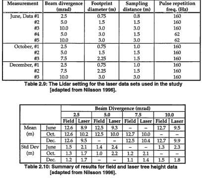
thinning, as shown in Table 2.9.

Tree heights were estimated using an algorithm that was initially developed for depth sounding. The results of the laser measurements were compared with the ground truth data. Both laser and ground data were transformed to a grid with a O.Sm resolution. To match both data sets, two methods were used. The first method used a correlation algorithm, which defined the correct position as the location with the highest correlation between the laser and field data (June data sets), whereas the second method used white plastic targets prior to laser data collection (October and December data sets).

Measurement Beam divergence Footprint Sampling Pulse repetition (mrad) diameter (m) distance (m) freq. (Hz)

June, Data #1 2.5 0.75 0.8 160

#2 5.0 1.5 1.5 160

#3 10.0 3.0 3.0 160

#4 5.0 3.0 1.5 62

#5 10.0 3.0 3.0 62

October,#1 2.5 0.75 1.0 160

#2 5.0 1.5 1.5 160

#3 7.5 2.25 1.5 160

December, #1 2.5 0.75 1.0 160

#2 7.5 2.25 1.5 160

#3 10.0 3.0 3.0 160

Table 2.9: The Lidar setting for the laser data sets used in the study [adapted from Nilsson 1996).

Beam Diverp·ence (mrad)

2.5 5.0 7.5 10.0

Field Laser Field Laser Field Laser Field Laser Mean June 12.6 8.9 12.5 9.3

-

-

(m) Oct. 12.6 10.2 12.5 10.0 12.7 10.0 -

-

(m) Oct. 1.3 1.7 1.0 2.2 1.2 2.1

-

-Dec. 1.2 1.7

-

-

Table 2.10: Summary of results for field and laser tree height data [adapted from Nilsson 1996).

Table 2.10. For the June data sets, the use of a larger footprint produced a higher mean height but this efect was not apparent for the October and December data sets.

Naesset (1997b) describes an investigation of the Optech ALTM 1020 laser scanning system. The aircraft was flown over an area of spruce and pine dominated forests (age ranging from 31 to 145 years) at 640-825m above the ground and at a

speed of 80m/s approximately. Laser data were collected with a maximum scan angle (off nadir) of 20°, which gave an average swath width of about 460-600m and side overlap between 70-425m. A beam divergence of 0.25 mrad was used, producing footprints with a diameter of approximately 13-16cm. The laser data were geo-referenced using differential GPS mounted on the plane, and were transformed into a local coordinate system to match with the digitised stand

boundaries. The results from laser measurements were compared with data obtained with conventional field measurements (Table 2.11).

Test No.of Stand area (ha) Tree species distribution (%) Height (m)

site stands Range Mean Spruce Pine Range Mean

1 2

18 0.7-4.6 1.5 3 97 8.1-24.3

18 0.5-3.4 1.5 69 28 8.2-20.1

Table 2.11: Summary of ground truth data [adapted from Naesset -1997b].

Test site Comparison D(m) SD(m)

1 At15mx15m -0.4 (P,,,O) 1.3

1 At20mx20m 0.3 (P,,,O) 1.3

1 At30mx30m 1.1 (P<0.01) 1.3

2 At15mx15m 0.1 (P,,,O) 1.2

2 At20mx20m 0.9 (P<0.01) 1.2

2 At30mx30m 1.9 (P<0.001) 1.3

17.5 14.9

Table 2.12: Mean difference (D= laser-ground data) between laser and

ground data and the standard deviation (SO) of the difference [adapted from Naesset 1997b].

The analysis was divided using two methods: original data analysis and grid analysis. For original data analysis, the laser mean height underestimated the ground height by 2.1-3.6m. For the grid analysis, both data sets were transformed

A pulsed near infrared laser system developed by NASA, and called SLICER (scanning lidar imager of canopies by echo recovery) was used to measure tree height of coniferous forests in the Pacific Northwest of the United States [Means et al. 1999]. The aircraft was flown approximately 5000m above the ground, producing large laser footprints, nominally lOm in diameter. A differential GPS receiver was mounted on the aircraft to determine aircraft position, allowing the horizontal position of the first reflecting surface of each pulse to be determined to within ±5 to ±lOm. SLICER data were compared with conventional field plot measurements (Table 2.13). The accuracy of matching the field plot and SLICER

footprints was estimated to be 5-20m.

Forest type No. of plots Density (trees/ha) Mean height (m)

Young 7 1975 17

Mature 5 948 33

Old-growth 9 689 43

Table 2.13: Summary of field plot data [adapted from Means et al.

1999].

Using a regression analysis, SLICER data correlated well with the field measured data (r2_{=0.95), with a RMSE of 3.8m. For tree heights more than about}

3m, heights derived from SLICER overestimated heights measured on the ground. Based on the given equation model, the amount of overestimation depends on tree height, from zero at 3m to about 9% at 50m (tree heights measured on the ground) [Acker 2000].

Laser systems have demonstrated potential for measuring terrain data and some forest parameters. In the case of tree heighting, depending on the size of the

2.6. Optical Satellites

Various space borne imaging spectrometers produce repetitive, small-scale synoptic images for measuring biophysical parameters and monitoring landscape change; for example, Landsat MSS and TM, SPOT, the Japanese Earth Resource Satellite (JERS-I), and the Indian Resource Satellite (IRS-IA, IB, and IC).

Landsat MSS data has been used to develop regression models for timber volume estimation in Scots pine dominated forest stands [Jaakkola and Sauk:kola I979], to estimate stocking in sparse to moderately stocked ponderosa pine forests [Strahler and Li I98I], to estimate the age and volume of stands [Poso et al. I984, I 987], and to assess continental or sub-continental forest resources in a stratified

sampling design [Nelson et al. I987].

Landsat TM data has been used to estimate volumes and age of stands [Poso et al. I984, I987], to relate biomass and successional age to vegetation index derived from TM data [Sader et al. I989], and to estimate above ground biomass on semiarid rangelands [Anderson et al. I993].

SPOT-I data has been used to estimate the stand age of radiata pine in Canberra, Australia [Turner et al. I987], and to estimate five stand variables (tree density, mean DBH, mean tree height, mean density and age) of Corsian pine in northern England [Danson I 987]. In the case of measuring tree height, Danson

(I987) found that the SPOT NIR data had strongly negative correlation with mean height (R=-0.83) but did not provide a detailed statistical summary.

2.7. Airborne Line lmagers

In forestry, CASI has been applied to the discrimination of forest species and canopy density [e.g. Franklin 1994], tree crown recognition and counting [e.g. Held and Billings 1998], and forest moisture stress mapping [e.g. Chisholm and Louis 1998]. The advantage of CASI over an airborne optical array sensor is its higher spectral resolution. Stereo viewing is possible but less convenient because it can only use viewing of side-lap between adjacent flight lines. No published

applications of airborne line imagers to tree heighting have been found.

2.8. Airborne Videography

Airborne video is captured continuously along a flight line, usually at 25 or 30 frames per second. The analog data in individual frames can be converted into digital data using a video frame grabbing board with image resolution limited to

about 792x480 pixel [Pitt et al. 1997], or stored digitally in the case of a digital video camera.

Compared to a film camera, videography provides much lower spatial resolution and requires a large number of frames for comparable results [Wright 1993]. Other limitations, depending on the method of image plane scanning, are poor and inconsistent image geometry and the addition of electronic noise [King and Vlcek 1990]. However, in some applications where the high resolution of photographic film is not required, video offers an affordable alternative because of its low cost, convenience, and immediate availability [King and Vlcek 1990].

2.9. Summary

Remote sensing techniques have been used to measure a range of forest parameters for inventory purposes using various methods and approaches. The techniques range from large-scale vegetation classification to measurement of individual tree characteristics.

In the case of measuring tree height, there are three competing technologies: aerial photography using photogrammetric techniques, airborne laser, and radar. These three technologies have a demostrated potential to compete with field measurement techniques. However, for inventory purposes, large format aerial photographs and photogrammetric techniques offer some important advantages to forest managers:

i. higher spatial resolution and accuracy, ii. superior stereo capability;

iii. potential to provide additional inventory data; and

iv. lower cost, with the photography already routinely acquired and used intensively by forest managers.

Techniques developed for aerial photography also offer the possibility to measure historical data (e.g. Long-term growth) using the exten&ive collections of large format aerial photographs held by most forestry organisations.

Previous research has demonstrated the potential of photogrammetric techniques to provide tree height data. This research focuses on the utility of aerial

Chapter 3. Image Matching Techniques

3.1. Introduction

Image matching plays a key role in the automation of digital photogrammetry. The technique can be used to supplement, complement or replace the human operator. In photogrammetry, matching is essential for two separate procedures; the first is image orientation, and the second is three-dimensional object reconstruction. The orientation processes require measurements of fiducial marks for interior orientation, pass points for relative orientation, and ground control points in absolute orientation. The second procedure is the determination of position and elevation of image points in the overlap area.

A digital photogrammetric workstation (DPW) consists of hardware and software to carry out photogrammetric tasks in an interactive and automated way using digital image data as input. The resulting photogrammetric products include three-dimensional coordinates, geometric and radiometric object surface descriptions, structured vector data, and transformed digital imagery (e.g. orthoimages and perspective views) [e.g. Griin 1989].

The characteristics and advantages of a DPW in comparison to analogue and analytical methods are [Grun 1989, Lohmann et al. 1990]:

• no need for high precision opto-mechanical parts, • robust measurement system,

• data acquisition, storage and processing in one system, • online and real time capabilities, and

• direct three-dimensional graphic superimposition possibilities.

Leading DPWs such as the Leica-Helava, BRDAS Imagine OrthoMAX, Autometric Softplotter, INPHO, Zeiss PHODIS, VirtuoZo, and Intergraph ImageStation (now Zll Imaging) systems offer complete photogrammetric functionality including orientations, aero triangulation, automatic DBM generation

and orthophoto production. This chapter reviews the image matching algorithms employed in these leading digital photogrammetric workstations. Comparative studies of their performances are reviewed, focusing on the performance of automatic DBM extraction.

3.2. Classification of Image Matching Techniques

Before discussing the matching techniques employed by different digital photogrammetric systems, it is appropriate to describe the range of matching techniques that have been developed. The following classification is based on four fundamental questions (see Vosselman 1992 for a similar approach):

(1) What primitives are being matched?

(2) What models are used to define the geometric and radiometric mapping between primitives?

(3) How is the match measured? (4) How is the best match found?

3.2.1. What Primitives are Being Matched?

There are two broad categories of matching primitives: windows composed of grey values, and features extracted from an image prior to matching. These two distinct categories lead to two different approaches to image matching: area based matching and feature based matching [Heipke 1992].

comprise the whole image.

3.2.1.1. Area Based Matching

In area based matching, small windows composed of grey values are used as matching primitives. The windows are normally square. The window on one image is used as a reference window (called the template window), while the corresponding window on the other image is called the search window. The template window centre, possibly weighted with respect to the grey value gradient, defines the point to be matched.

The advantage of area based matching is that high accuracy can be achieved in well-textured image regions. Accuracy comparable to human operator based measurements have been reported [e.g. Pertl 1985, Griin and Baltsavias 1987,

Rosenholm 1987a]. The disadvantages of area based matching include the sensitivity of the grey values to changes in radiometry, and the time required for searching for the best match.

3.2.1.2. Feature Based Matching

Feature based matching determines the correspondence between image features. In feature based matching, features such as points, lines and regions are extracted from both images prior to matching. Features selected for matching must have the following characteristics [Forstner 1986]:

• Distinctness: The selected point should be distinct from the neighbouring points, ensuring local separability.

• Invariance: The distinct point position should be invariant with respect to the expected geometric and radiometric distortions.

• Stability: The selected point should be robust with respect to noise and be expected to appear in the other image.

• Seldomness: Seldomness aims at global separability.

• Interpretability: The selection should be interpretable, for example, identifying edges, comers or other simple features.

Beside the attributes of features, the relationship between local features is introduced to characterise global features. These can be geometric or radiometric. Geometric relationships can be, for example, the angle between two adjacent polygons or the minimum distance between two edges. Radiometric relationships can be, for example, the difference in grey value between two adjacent polygons. A description of primitives and their interrelationship is called a relational description [Vosselman 1992: 7].

Local features have been used for matching by, for example, Forstner (1986) and Hannah (1989), where in each case, points were selected as features. Global features are usually composed of local features. Matching with global features is referred to as relational matching [Shapiro and Haralick 1987]. Relational matching using global features has been described by, for example, Vosselman (1992). A combination of global and local features is described by Schenk et al.

(1991).

One of the advantages of feature based techniques are that they are faster than area based techniques, because the number of matched elements is generally lower. The other advantage is that they have a reduced sensitivity to light variations and, in general, to all radiometric differences between images of the stereo pair, because the criteria for matching are mainly geometric and structural rather than based on similarity of the neighbouring pixels [Cappelini et al. 1991]. The disadvantages are lower accuracy, and poorer indication of the quality of the match.

3.2.2. What Models are Used to Define the Geometric and

Radiometric Mapping Between Primitives?

The mapping between the primitives of the various images can be defined using a sensor model, an object surface model or a combination of the two.

3.2.2.1. Sensor Models and the Epipolar Constraint