Development of measurement-based load models for the dynamic simulation of distribution grids

Development of measurement-based load models

for the dynamic simulation of distribution grids

Eleftherios O. Kontis, Mazheruddin H. Syed, Efren Guillo-Sansano Theofilos A. Papadopoulos,

Andreas I. Chrysochos, Grigoris K. Papagiannis, Graeme M. Burt

978-1-5386-1953-7/17/$31.00 c2017 IEEE

Abstract—The advent of new types of loads, such as power electronics and the increased penetration of low-inertia motors in the existing distribution grids alter the dynamic behavior of conventional power systems. Therefore, more accurate dynamic, aggregate, load models are required for the rigorous assessment of the stability limits of modern distribution networks. In this paper, a measurement-based, input/output, aggregate load model is proposed, suitable for dynamic simulations of distribution grids. The new model can simulate complex load dynamics by employing variable-order transfer functions. The minimum required model order is automatically determined through an iterative procedure. The applicability and accuracy of the pro-posed model are thoroughly evaluated under distinct loading conditions and network topologies using measurements acquired from a laboratory-scale test setup. Furthermore, the performance of the proposed model is compared against other conventional load models, using the mean absolute percentage error.

Index Terms—Distribution grids, dynamic equivalencing, measurement-based approach, system identification techniques.

I. INTRODUCTION

Despite the research efforts from both academia and indus-try, modeling of distribution grids remains a very challenging task [1]. The vast number of different individual electric and electronic devices in distribution networks and their time-varying, stochastic nature pose several difficulties in the al-ready complex modeling procedure [2]. To overcome these issues, aggregated load models are typically adopted by system operators [3].

The load modeling challenge is to determine an equivalent representation for the aggregation of different types of indi-vidual components, supplied by a common busbar [4], [5].

The work in this paper has been supported by the European Commission, under the FP7 project ELECTRA (grant no: 609687) and Horizon 2020 project ERIGrid (grant no: 654113). Any opinions, findings, and conclusions or recommendations expressed in this material are those of the authors and do not necessarily reflect those of the European Commission.

Eleftherios O. Kontis, and Grigoris K. Papagiannis are with the Power Systems Laboratory, School of Electrical and Computer Engineering, Aris-totle University of Thessaloniki, Thessaloniki, Greece, GR 54124, (e-mail: [email protected]; [email protected]).

Theofilos A. Papadopoulos is with the Power Systems Laboratory, Dept. of Electrical and Computer Engineering, Democritus University of Thrace, Xanthi, Greece, GR 67100, (e-mail: [email protected]).

Andreas I. Chrysochos is with the CablelR _{Hellenic Cables S.A., Viohalco}

Group, Sousaki Korinthias, Korinthos, Greece, GR 20100 (e-mail: [email protected]).

Mazheruddin H. Syed, Efren Guillo-Sansano, and Graeme M. Burt are with the Institute for Energy and Environment University of Strath-clyde, Glasgow, UK (e-mail: [email protected]; [email protected]; [email protected]).

Generally, load modeling procedure consists of two dinstinct stages. In the first stage, a suitable load model structure is defined, while in the second stage the required model parameters are estimated [3].

The choice of the model structure depends on the needs of the analysis, the expected accuracy, and the load composition. Therefore, load models are divided into two main categories: Static and dynamic models [2], [3]. Static load models describe the relationship between load real/reactive power, voltage and/or frequency at any time instant using algebraic equations. Static models can be used for loads that do not exhibit signifi-cant dynamic response after a disturbance [6] or when analysis of the equilibrium conditions is only considered [7]. In case of voltage and angular stability analysis, dynamic load models are required. Dynamic models describe the relationship between load real/reactive power at any time instant as functions of voltage and/or frequency of the present and past time instants [8]. Difference or differential equations are used to describe such models.

Once the model structure is specified, the remaining task focuses on the estimation of the required model parameters. For this purpose, the component- and the measurement-based approaches can be used. The implementation of component-based methodology requires reliable information of the load class mix, the load components as well asa prioriknowledge of typical characteristics of individual devices [8]. Therefore, the application of this method requires accurate data, which usually cannot be determined in distribution networks due to their size and confidentiality [9]. On the other hand, in the measurement-based approach the required model parameters are estimated from in-situ measurements, using parameter identification techniques [2], [10]. This method directly cap-tures the actual load dynamics, resulting in more accurate models. Moreover, when new measurements are available, the required model parameters can be easily updated close to real-time, enhancing the accuracy of the developed models [6], [8]. The aforementioned advantages in conjunction with the increased availability of measurements due to the installation of phasor measurement units (PMUs) at distribution level, constitute the measurement-based approach more appealing compared to the component-based methodology [11].

new model employs variable-order transfer functions for the modeling of the recovery phase of the load. Thus, it can reproduce accurately complex dynamic phenomena caused by power electronic loads and motor drives. The accuracy and effectiveness of the proposed model are evaluated using measurements acquired from a laboratory-scale test setup. Furthermore, its performance is thoroughly compared with other conventional load models.

Following this introduction, the remaining of the paper is organized as follows: In Section II, an overview of the ERLM is presented. The mathematical formulation of the proposed dynamic load model and the corresponding parameter esti-mation procedure are explained in Section III. Section IV describes the examined laboratory setup. The performance of the proposed model is evaluated in Section V, while in Section VI sensitivity analysis is performed. Finally, Section VII concludes the paper.

II. THEORETICALBACKGROUND

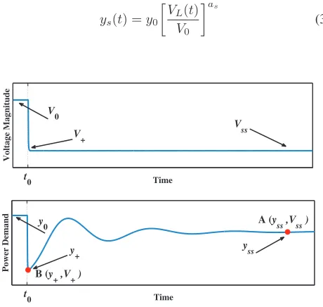
The general dynamic response of conventional power sys-tem loads is presented in Fig. 1. As shown, immediately after a voltage disturbance, the load consumption decreases instantaneously to y+ value. After the transient overshoot a

recovery phase occurs. During this phase the load demand gradually recovers to a new steady-state value, i.e. to yss.

To simulate this dynamic behavior, Hill and Karlsson pro-posed the use of the ERLM [12], [13], the mathematical representation of which is defined as:

Tyy˙r(t) +yr(t) =ys(t)−yt(t) (1)

yl(t) =yr(t) +yt(t) (2)

where yl denotes the total load demand in real or reactive

power at time t, yr is the recovery state of the load, ys

andyt are two auxiliary functions describing the steady-state

and transient characteristics of the load, respectively. These functions are defined as:

ys(t) =y0

_V

L(t)

V0

as

(3)

Time

Voltage Magnitude

Time

Power Demand

V

+

y

ss

V

ss

A (y

ss ,Vss )

y

+

y

0

V

0

t

0

t

0

B (y

+ ,V+ )

Fig. 1. Typical response of conventional power system loads.

V

N1 (s) G (s)

N2 (s)

yl(t)

L-1_{N

1 (s) G (s)}=yr (t)

Σ

L-1_{N

2 (s)}=yt (t)

Fig. 2. Block diagram representation of the ERLM.

y_t(t) =y₀

_V

L(t)

V₀

at

(4)

WhereV0and y0denote the voltage magnitude and power

consumption prior to the disturbance as shown in Fig. 1,VL(t)

is the measured load voltage, as and at are the steady-state and transient voltage exponents, respectively. The values ofas

andatcan be calculated from the operating pointsA(yss, Vss)

andB(y+, V+), using the following algebraic equations:

as=

log

yss y0

log

Vss V0

at=

log

y+ y0

log

V+ V0

(5)

By introducing the following simplifications:

N₁(t) =y_s(t)−y_t(t) (6)

N2(t) =yt(t) (7)

Eqs. (1) and (2) can be rewritten as:

Tyy˙r(t) +yr(t) =N1(t) (8)

yl(t) =yr(t) +N2(t) (9)

By applying the Laplace transform and performing some simple manipulations, (8) and (9) can be rewritten as:

yr(s) =N1(s)·_{s+ 1}1/T_/Ty

y (10)

yl(s) =N2(s) +N1(s)·_{s+ 1}1/T_/Ty

y (11)

The block structured representation of (10) and (11) is presented in Fig. 2. As shown, the ERLM can be perceived as a block diagram interconnection of two nonlinear, exponential functions and a first-order linear transfer function. The gain of this transfer function is equal to1/Ty, while the corresponding

pole is−1/Ty.

III. PROPOSEDEQUIVALENTMODEL

To develop the proposed model, the block diagram repre-sentation of Fig. 2 is extended by employing high-order linear transfer functions, with general form as:

G(s) = β_sν_μsν₊+_αβν−1sν−1+...+β0 μ−1sμ−1+...+α0 =

μ

m=1

cm

s−pm (12)

In this case, the only restriction is that the G(s) function must be strictly proper, i.e., ν < μ, to ensure that the recovery of the load is continuous [12], [13]. Generally, the required set of parameters θ= [p,c] can be estimated using parameter identification techniques [14], [15]. In this paper,θ is identified using the vector fitting (VF) method [16]–[18], and the optimal order of the employed transfer functions is determined using the iterative procedure of Algorithm 1.

When a voltage disturbance occurs, the resulting load and voltage responses are recorded and used for the estimation of the required model parameters. Initially, voltage exponents

as andat are determined from (5). Afterwards, functionsN1

andN2are computed in time-domain (TD) using (6) and (7),

respectively. Subsequently, the recovery response of the load, i.e. yr, is calculated in TD using (2). The Laplace transform

(LT) of signals N1 andyr is calculated and the response of

the characteristic transfer function G(s) is extracted in the frequency domain (FD):

G(s) = _LL₍(_Nyr(t))

1(t)) (13)

This response is approximated with a linear transfer func-tion, denoted as Gˆ(s). To determine the minimum required order of Gˆ(s), the following iterative procedure, is adopted: In each iteration, the order of Gˆ(s)is increased by one and the required set of parameters θn is identified using the VF method. Here, n denotes the n-th iteration of the algorithm and initially is set to one. Subsequently, as shown in Fig. 2, the estimated load response is calculated in TD using (14).

yest(t) =N2(t) +L−1[N1(s) ˆG(s)] (14)

Then, yest is compared with the actual load response yl,

with mean value y¯l, and the following validation index is

calculated:

R2

n=

1−

M

m=1(yl[m]−yest[m|θn])2

M

m=1(yl[m]−y¯l)2 ·100%

(15)

where M denotes the total number of TD samples. Finally, the ΔR2 = R2_n − R2_n−1 criterion, between the last two successful iterations is computed. For the first iteration, R2₀ is set equal to zero. If the value of the ΔR2 coefficient is less than a predefined tolerance, the proposed modeling procedure terminates, resulting to a model order no=n−1

[19]. Otherwise, a higher order approximation for theG(s)is computed.

IV. SYSTEMUNDERSTUDY

To validate the applicability of the proposed model, a series of laboratory tests were conducted at the Dynamic Power

Algorithm 1Pseudocode for the proposed modeling procedure 1: Acquire a set of measurement data, i.e.VL(t)andyl(t).

2: Determineas andat parameters, using (5).

3: CalculateN1 andN2in TD, using (6) and (7).

4: Computeyr in TD, using (2).

5: Calculate the LT ofN1andyr.

6: Extract theG(s)function in FD, using (13). 7: Determine the desired tolerance, i.e.tol. 8: Setn= 0andR2₀= 0.

9: repeat 10: n=n+ 1.

11: Calculate ann-order approximation for the G(s) function using the VF algorithm.

12: Determine theyest response in TD, using (14).

13: Calculate theR2_n value. 14: Compute theΔR2 criterion. 15: untilΔR2 is less thantol.

16: Finalize model with order equal ton−1.

System Laboratory at University of Strathclyde. The test setup is comprised of a three-phase, 64-step, 10 kVA static load bank (SLB) connected in parallel with three induction motors, as shown in Fig. 3. Using this setup, two different network topologies were examined by switching on and off switchS1,

respectively. Moreover, for each topology, five distinct load compositions were considered and examined by changing the nominal power of the SLB. Thus, as summarized in Table 1, a set of ten distinct network configurations were implemented and used to evaluate the performance of the proposed model. The test setup is supplied by a three-phase programmable voltage source (PVS), allowing for instantaneous step-down voltage disturbances to be implemented. In all cases, a−6 % voltage disturbance was introduced and the corresponding voltage signals, the resulting real and reactive power responses at the point of common coupling (PCC) were recorded at a rate of500samples per second (sps). The acquired responses were used for the development and assessment of the proposed model.

M1

Program mabl e Voltage Source (PVS)

PCC

S1

St ati c Load Bank (SLB) 10 kVA Inducti on Motor

5.5 kVA

M2

M3

Inducti on Motor 7.5 kVA

Inducti on Motor 7.5 kVA 1st _{Exam ined t opology}

2n d _Examined

topology

TABLE I

SYNOPSIS OF THE EXAMINED CONFIGURATIONS

Examined

Configurations

Connected Elements

SLB M1 M2 M3

C1.1 2.114 kw, pf=0.9 ON ON ON

C1.2 4.077 kw, pf=0.9 ON ON ON

C1.3 6.040 kw, pf=0.9 ON ON ON

C1.4 8.003 kw, pf=0.9 ON ON ON

C1.5 9.513 kw, pf=0.9 ON ON ON

C2.1 2.114 kw, pf=0.9 ON OFF OFF

C2.2 4.077 kw, pf=0.9 ON OFF OFF

C2.3 6.040 kw, pf=0.9 ON OFF OFF

C2.4 8.003 kw, pf=0.9 ON OFF OFF

C2.5 9.513 kw, pf=0.9 ON OFF OFF

V. MODELEVALUATION

The accuracy of the proposed load model is thoroughly compared against the well-established ERLM, the exponential (EXP) [20] and the polynomial (ZIP) [20] load models, which are mostly used by distribution system operators for stability studies [21].

The parameters of the proposed model are estimated from the acquired measurements using the modeling procedure of Algorithm 1. On the other hand, the parameters for the conventional load models are determined using non-linear least square (NLS) optimization, targeting to minimize the following objective function [3].

J(p) = M

m=1

(yl[m]−yˆ[m])2 (16)

WhereM denotes the total TD samples,p is the required set of parameters, whileyˆ[m]denotes the estimated load response at the m-th sample.

To quantify the accuracy of the examined load models, the mean absolute percentage error (MAPE(%)) is used [7]:

MAP E(%) = 100_M M

m=1

yl[m]−yˆ[m]

yl[m]

(17)

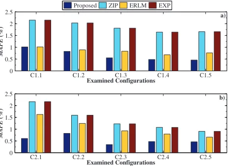
The calculated MAPEs for all examined configurations are summarized in Figs. 4 and 5.

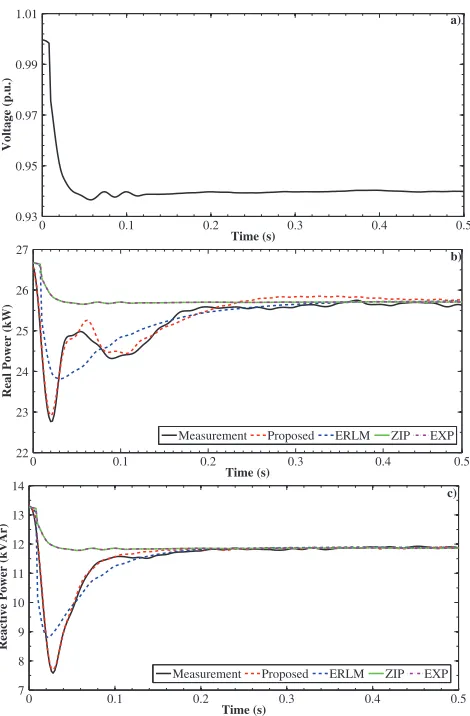
The performance of the considered models is further ana-lyzed in Figs. 6 and 7, where the measured real and reactive power responses are compared with the corresponding estima-tions, provided by the examined models.

In the first examined topology, after the power overshoot, caused by the instantaneous voltage drop, both real and reactive power recover to the new steady-state exponentially. On the other hand, in the second examined topology, both real and reactive power present an oscillatory behavior during the recovery period.

Based on the presented results it is clear that the EXP and ZIP load models fail to simulate adequately the dynamic

C1.1 C1.2 C1.3 C1.4 C1.5

0 0.5 1 1.5 2 2.5

Examined Configurations

MAPE

(%)

C2.1 C2.2 C2.3 C2.4 C2.5

0 0.5 1 1.5 2 2.5

Examined Configurations

MAPE

(%)

Proposed ZIP ERLM EXP

a)

b)

Fig. 4. MAPE (%) for the modeling of the real power. Configurations derived from the a) first and b) second topology.

C1.1 C1.2 C1.3 C1.4 C1.5

0 1 2 3 4 5 6

Examined Configurations

MAPE

(%)

C2.1 C2.2 C2.3 C2.4 C2.5

0 2 4 6 8 10

Examined Configurations

MAPE

(%)

Proposed ZIP ERLM EXP

a)

b)

Fig. 5. MAPE (%) for the modeling of the reactive power. Configurations derived from the a) first and b) second topology.

behavior of both real and reactive power. Indeed, due to the fact that both EXP and ZIP are static models, they can accurately estimate only the new steady-state power of the load. This is demonstrated in Figs. 6 and 7 and further verified by the corresponding MAPEs, depicted in Figs. 4 and 5. Therefore, it can be concluded that these models are not appropriate to be used for the dynamic analysis of distribution grids.

On the other hand, the ERLM can describe with higher accuracy, compared to the ZIP and EXP models, the dynamic behavior of the load, since in all examined cases considerably lower MAPEs are calculated. Moreover, as shown in Figs. 6 and 7, the ERLM can estimate very accurately the new steady-state of both real and reactive power, capturing also adequately the power overshoot. However, the first-order ERLM cannot replicate the oscillatory behavior of the load.

0 0.1 0.2 0.3 0.4 0.5 0.93

0.95 0.97 0.99 1.01

Time (s)

Voltage (p.u.)

a)

0 0.1 0.2 0.3 0.4 0.5

22 23 24 25 26 27

Time (s)

Real Power (kW)

Measurement Proposed ERLM ZIP EXP

b)

0 0.1 0.2 0.3 0.4 0.5

7 8 9 10 11 12 13 14

Time (s)

Reactive Power (kVAr)

Measurement Proposed ERLM ZIP EXP

c)

Fig. 6. Comparative assessment of the derived models for C1.3 configuration. a) Examined voltage disturbance. Modeling of b) real power and c) reactive power.

MAPEs in all examined cases are lower than1.02%, while for the modeling of the reactive power MAPEs smaller that1.38% are observed. The effectiveness of the proposed model is also qualitatively verified by the results depicted in Figs. 6 and 7. The developed model can simulate the dynamic behavior of both the real and reactive power, capturing accurately the overshoot, the recovery phase and the new steady-state of the load.

VI. SENSITIVITYANALYSIS

A sensitivity analysis is performed using the dynamic re-sponses acquired from C1.3 and C2.3 configurations. Scope of the analysis is to investigate the influence of the model parameters on the accuracy of the simulated responses.

Initially, four discrete sets of optimal model parameters are determined using the proposed modeling procedure, describing the real and reactive power of C1.3 and C2.3 configura-tions. Next, sensitivity analysis is performed by introducing intentionally to each model parameter a 10% and 20% error from the original value. The resulting MAPEs are presented in Tables II and III. Higher MAPE values indicate higher

0 0.1 0.2 0.3 0.4 0.5

0.93 0.95 0.97 0.99 1.01

Time (s)

Voltage (p.u.)

a)

0 0.1 0.2 0.3 0.4 0.5

9.4 10.4 11.4

Time (s)

Real Power (kW)

Measurement Proposed ERLM ZIP EXP

b)

0 0.1 0.2 0.3 0.4 0.5

3.5 4.5 5.5 6.5

Time (s)

Reactive Power (kVAr)

Measurement Proposed ERLM ZIP EXP

c)

Fig. 7. Comparative assessment of the derived models for C2.3 configuration. a) Examined voltage disturbance. Modeling of b) real power and c) reactive power.

TABLE II

MAPES WITH VARIATION IN MODEL PARAMETERS. RESULTS FORC1.3

CONFIGURATION.

Modeling of real power Modeling of reactive power

Error in model parameters Error in model parameters

0% 10% 20% 0% 10% 20%

as 0.5527 0.7631 1.0231 0.4581 1.2117 2.0610

at 0.5527 0.5841 0.7385 0.4581 0.6337 0.8477

p 0.5527 0.6299 0.8071 0.4581 0.7217 0.9692

c 0.5527 0.6361 0.8412 0.4581 0.5919 1.0550

influence of the corresponding model parameter. Results show that erroneous values of the steady-state voltage exponent, i.e.

a_s, result in the highest MAPEs, indicating the significant impact of this parameter on the model accuracy. Additionally, it is clear that the poles of theG(s)function, i.e.p, have also a significant effect on the model performance, while the transient voltage exponent, i.e.at, is the least influential parameter.

TABLE III

MAPES WITH VARIATION IN MODEL PARAMETERS. RESULTS FORC2.3

CONFIGURATION.

Modeling of real power Modeling of reactive power

Error Error

0% 10% 20% 0% 10% 20%

as 0.3477 0.4910 1.0865 1.2446 2.2734 3.5455

at 0.3477 0.3565 0.4761 1.2446 1.4486 1.7397

p 0.3477 0.5462 0.7732 1.2446 1.8809 2.6196

c 0.3477 0.3765 0.5202 1.2446 1.3108 1.5688

ZIP and EXP models even in cases where highly erroneous parameters are considered. This can be verified by the corre-sponding MAPE values, presented in Figs. 4 and 5. Specif-ically, concerning the modeling of real and reactive power for C1.3 configuration, both ZIP and EXP models result in MAPEs higher than 1.8% and 4.1%, respectively, while for C2.3 configuration the corresponding MAPEs are higher than 1.23% and 3.06%.

VII. CONCLUSIONS AND FUTURE WORK

In this paper, a measurement-based, input/output, aggregate load model is proposed for the dynamic analysis of distri-bution systems. The proposed model is based on the well-established ERLM, however, contrary to the conventional first-order ERLM, the proposed model uses variable-first-order linear transfer function to simulate accurately the recovery phase of the load.

The accuracy and applicability of the proposed model are thoroughly evaluated under different, distinct network con-figurations using measurements acquired from a laboratory-scale test setup. In all examined cases, the experimental results indicate that the developed model can capture very accurately the dynamic behavior of the load. Moreover, the performance of the proposed model is compared with the conventional ERLM, as well as with the static ZIP and EXP models. Additionally, a sensitivity analysis is performed to investigate the impact of the model parameters in the resulting accuracy. The sensitivity analysis in conjunction with the comparative assessment highlight the superior performance of the proposed model compared to the conventional approaches.

Future work will be conducted to validate the performance of the proposed model under different network configurations and voltage disturbances and to determine the most accurate system identification technique to estimate the parameters of theG(s)function. Finally, the ability of the developed model to simulate the dynamic behavior of distribution networks with high penetration levels of distributed renewable energy sources will be also investigated.

REFERENCES

[1] D. P. Stojanovic, L. M. Korunovic, and J. Milanovic, “Dynamic load modelling based on measurements in medium voltage distribution net-work,”Elect. Power Syst. Res., vol. 78, no. 2, pp. 228 – 238, Feb 2008.

[2] V. Knyazkin, C. A. Canizares, and L. H. Soder, “On the parameter estimation and modeling of aggregate power system loads,”IEEE Trans. Power Syst., vol. 19, no. 2, pp. 1023–1031, May 2004.

[3] B.-K. Choi, H.-D. Chiang, Y. Li, H. Li, Y.-T. Chen, D.-H. Huang, and M. G. Lauby, “Measurement-based dynamic load models: derivation, comparison, and validation,”IEEE Trans. Power Syst., vol. 21, no. 3, pp. 1276–1283, Aug 2006.

[4] I. F. Visconti, D. A. Lima, J. M. C. d. S. Costa, and N. R. d. B. C. So-brinho, “Measurement-based load modeling using transfer functions for dynamic simulations,”IEEE Trans. Power Syst., vol. 29, no. 1, pp. 111– 120, Jan 2014.

[5] E. O. Kontis, A. I. Chrysochos, G. K. Papagiannis, and T. A. Pa-padopoulos, “Development of measurement-based generic load models for dynamic simulations,” in2015 IEEE Eindhoven PowerTech, June 2015, pp. 1–6.

[6] P. Regulski, D. S. Vilchis-Rodriguez, S. Djurovic, and V. Terzija, “Estimation of composite load model parameters using an improved particle swarm optimization method,”IEEE Trans. Power Del., vol. 30, no. 2, pp. 553–560, April 2015.

[7] A. Miranian and K. Rouzbehi, “Nonlinear power system load identifi-cation using local model networks,”IEEE Trans. Power Syst., vol. 28, no. 3, pp. 2872–2881, Aug 2013.

[8] Konstantinos S. Metallinos, Theofilos A. Papadopoulos, and Char-alambos A. Charalambous, “Derivation and evaluation of generic measurement-based dynamic load models,”Elect. Power Syst. Res., vol. 140, pp. 193 – 200, 2016.

[9] P. Jazayeri, W. Rosehart, and D. T. Westwick, “A multistage algorithm for identification of nonlinear aggregate power system loads,” IEEE Trans. Power Syst., vol. 22, no. 3, pp. 1072–1079, Aug 2007. [10] E. O. Kontis, T. A. Papadopoulos, A. I. Chrysochos, and G. K.

Papagiannis, “Measurement-based dynamic load modeling using the vector fitting technique,”Trans. Power Syst., Early Access.

[11] H. Bai, P. Zhang, and V. Ajjarapu, “A novel parameter identification approach via hybrid learning for aggregate load modeling,”IEEE Trans. Power Syst., vol. 24, no. 3, pp. 1145–1154, Aug 2009.

[12] D. Karlsson and D. J. Hill, “Modelling and identification of nonlinear dynamic loads in power systems,”IEEE Trans. Power Syst., vol. 9, no. 1, pp. 157–166, Feb 1994.

[13] D. J. Hill and I. A. Hiskens, “Dynamic analysis of voltage collapse in power systems,” inDecision and Control, 1992., Proceedings of the 31st IEEE Conference on, 1992, pp. 2904–2909 vol. 3.

[14] D. J. Trudnowski and J. W. Pierre, “Overview of algorithms for estimating swing modes from measured responses,” in2009 IEEE Power Energy Society General Meeting, July 2009, pp. 1–8.

[15] T. A. Papadopoulos, E. O. Kontis, P. N. Papadopoulos, and G. K. Pa-pagiannis, “System identification techniques for power systems analysis using distorted data,” inMedPower 2014, Nov 2014, pp. 1–7. [16] B. Gustavsen and A. Semlyen, “Rational approximation of frequency

domain responses by vector fitting,”IEEE Trans. Power Del., vol. 14, no. 3, pp. 1052–1061, Jul 1999.

[17] B. Gustavsen, “Improving the pole relocating properties of vector fitting,”IEEE Trans. Power Del., vol. 21, no. 3, pp. 1587–1592, July 2006.

[18] T. A. Papadopoulos, A. I. Chrysochos, E. O. Kontis, and G. K. Papagiannis, “Ringdown analysis of power systems using vector fitting,”

Elect. Power Syst. Res., vol. 141, pp. 100 – 103, 2016.

[19] T. A. Papadopoulos, A. I. Chrysochos, E. O. Kontis, P. N. Papadopou-los, and G. K. Papagiannis, “Measurement-based hybrid approach for ringdown analysis of power systems,”IEEE Trans. Power Syst., vol. 31, no. 6, pp. 4435–4446, Nov 2016.