City, University of London Institutional Repository
Citation
:
Banerjee, J. R., Papkov, S.O., Liu, X. and Kennedy, D. (2015). Dynamic stiffness matrix of a rectangular plate for the general case. JOURNAL OF SOUND AND VIBRATION, 342, doi: 10.1016/j.jsv.2014.12.031This is the accepted version of the paper.
This version of the publication may differ from the final published
version.
Permanent repository link: http://openaccess.city.ac.uk/14357/
Link to published version
:
http://dx.doi.org/10.1016/j.jsv.2014.12.031Copyright and reuse:
City Research Online aims to make research
outputs of City, University of London available to a wider audience.
Copyright and Moral Rights remain with the author(s) and/or copyright
holders. URLs from City Research Online may be freely distributed and
linked to.
City Research Online: http://openaccess.city.ac.uk/ [email protected]
DYNAMIC STIFFNESS MATRIX OF A RECTANGULAR PLATE FOR THE GENERAL CASE
J.R. Banerjeea*, S.O. Papkovb, X. Liua, D. Kennedyc
a
School of Engineering and Mathematical Sciences, City University London, London EC1V 0HB, UK
b
Department of Mathematics, Sevastopol National Technical University, Sevastopol 99053, Ukraine
c
School of Engineering, Cardiff University, Cardiff CF24 3AA, Wales, UK
Abstract
The dynamic stiffness matrix of a rectangular plate for the most general case is developed by solving the
bi-harmonic equation and finally casting the solution in terms of the force-displacement relationship of the freely
vibrating plate. Essentially the frequency dependent dynamic stiffness matrix of the plate when all its sides are
free is derived, making it possible to achieve exact solution for free vibration of plates or plate assemblies
with any boundary conditions. Previous research on the dynamic stiffness formulation of a plate was restricted
to the special case when the two opposite sides of the plate are simply supported. This restriction is quite
severe and made the general purpose application of the dynamic stiffness method impossible. The theory
developed in this paper overcomes this long-lasting restriction. The research carried out here is basically
fundamental in that the bi-harmonic equation which governs the free vibratory motion of a plate in harmonic
oscillation is solved in an exact sense, leading to the development of the dynamic stiffness method. It is
significant that the ingeniously sought solution presented in this paper is completely general, covering all
possible cases of elastic deformations of the plate. The Wittrick-Williams algorithm is applied to the ensuing
dynamic stiffness matrix to provide solutions for some representative problems. A carefully selected sample
of mode shapes is also presented.
Keywords: Dynamic stiffness method; free vibration; classical plate theory; bi-harmonic equation; arbitrary boundary conditions
*
2 Nomenclature
w transverse displacement
h, 2a, 2b thickness and dimensions of the rectangular plate
ω, Ω circular frequency and frequency parameter
E, ,, D Young’s modulus, Poisson ratio, density and bending stiffness of the plate W, y,
x amplitudes of transverse displacement and bending rotations on the boundariesVx, Vy, Mx, My amplitudes of shear forces and bending moments on the boundaries
d
~
,~
f
amplitudes of boundary displacement and force vectorsn , n
, wave numbers for the symmetric components of displacements
n n
~ ,
~
, wave numbers for the antisymmetric components of displacementsn n n n
,
p
,
q
,
q
p
1 2 1 2 roots of the characteristic equation(k,j) indicators ofsymmetric/antisymmetric componentswith k,j{0,1}
n n n n B C D
A, , , unknown coefficients of the general solution
W
,φ
,M
,V sequence vectors of Fourier coefficients for displacements, rotations, bending moments and shear forces at the boundariesQ
P
A
,
,
coefficient matrices in the mixed formulationd
,f
Fourier coefficients of the amplitudes of displacement and force vectorsK
dynamic stiffness matrixj
G asymptotic constant in limitant analysis
j
number of eigenvalues between zero and a trial frequency0
3 1. Introduction
The free vibration analysisof plates and plate assemblies is a topic which has continually inspired researchers
for well over two centuries. From an engineering perspective, the importance of this topic cannot be over
emphasized, particularly for its applications in aeronautical industry where the top and bottom skins of an
aircraft wing are generally idealised as plate assemblies during the structural design. Researchers who laid the
foundation for the current state of the art on the subject include Chladni [1], Poisson [2], Lord Rayleigh [3],
Ritz [4], Timoshenko [5] and Iguchi [6], amongst others. These early pioneers developed analytical methods,
later referred to as classical methods, at a time when the finite element method (FEM) was not even invented
and the computer power was almost non-existent. Then with the advent and rapid growth of powerful digital
computers, the FEM emerged in the 1960s as a breakthrough in solid mechanics and it became possible to
obtain approximate solutions for static and dynamic problems of structures such as beams, plates and their
assemblies through the use of assumed shape functions. During this period, interest in classical methods
continued and in fact was growing steadily to validate and importantly, to give due recognition and
importance to the FEM and to put it on a reliable, but secure foundation. It was natural and understandable
that classical methods which rely on the solution of the governing differential equations were
comprehensively used at the time to validate the FEM. Logically the classical methods provided the ultimate
benchmark to the solution of the plate vibration problem and thus became an indispensable aid to validate the
FEM which is basicallya numerical method. For a better insight into the problem, Leissa [7, 8] recognised the
continuing need for the development of the classical methods and provided a comprehensive coverage of the
free vibration analysis of rectangular plates. By and large his methods relied on the solution of the differential
equation governing the plate motion undergoing free vibration, but they were not sufficiently general to cover
all possible boundary conditions of the plate in an exact sense when arriving at the solution. Other notable
contributors who used analytical approach, but applied different methods other than the FEM, are Warburton
[9], Gorman [10], Azimi et al [11], Bhat [12], Cheung and Kong [13], and Xing and Liu [14, 15]. There are
some excellent texts which elucidate the classical theories of plates [16-18].
Against the above background, it is useful to note that an elegant and powerful alternative to the FEM and
classical methods in free vibration analysis exists, but relatively unknown which is notably the dynamic
stiffness method (DSM). The method gives exact results like some of the classical methods, but has the added
advantage of handling complex structures for which individual element stiffness matrices comprising the
structure can be assembled to provide solutions for the whole structure. The basic building block in the DSM
is the frequency dependent dynamic stiffness (DS) matrix of a structural element. The DS matrix is generally
obtained from the exact solutions of the governing differential equations of the structural element undergoing
free vibration. The solutions are essentially exact shape functions which, unlike the FEM, are not based on
assumed interpolation polynomials to define the element deformation. Thus the accuracy achieved in the DSM
4
frequencies can be computed, even from a single structural element to any desired accuracy which of course,
is impossible in the FEM or in any other approximate methods. When dissimilar elements are used in the
DSM to model a complex structure, the DS elements are assembled in the usual way like the FEM, leading to
an eigenvalue solution procedure for computing natural frequencies and mode shapes. In such cases, there will
be no loss of accuracy, and the results from the DSM for the complex structure will still be exact. This is in
sharp contrast to FEM for which the results are not exact because of the assumptions made in the shape
functions.
For beam elements, the DSM is well established [19-21] and notably software based on the DSM is available
[22, 23] for exact free vibration analysis of skeletal structures. For a plate element, the DSM was first
developed by Wittrick and Williams [24] for plates and plate assemblies in the early seventies by using
classical theory. This was a significant achievement at that time and the theory was implemented in a program
called VIPASA [24]. However, their work was restricted to thin plates for which two opposite sides must be
simply supported. Thus the deflection of the plate was assumed to vary sinusoidally in the longitudinal
direction. In 1983, Williams and Anderson [25] made significant extension to the work of Wittrick and
Williams [24] by introducing Lagrangian multipliers to deal with rigid and/or elastic point supports on the
plate and they produced an enhanced computer code VICON [26]. Following this work, optimum design
features were added to form a new version of the program, called VICONOPT [27]. Two decades later,
Boscolo and Banerjee [28-30] extended the DS plate theory by including the important effects of shear
deformation and rotatory inertia. Their investigations cover both isotropic plates [28] and composite plates
[29, 30] and were based on the first-order shear deformation theory. Fazzolari et al took a step further to
develop the dynamic stiffness theory for anisotropic plates [31] using higher order shear deformation theory.
Later, Boscolo and Banerjee [32] developed DSM using sophisticated first-order layer-wise theory for the
analysis of laminated composite plates. However, all these investigations were limited to simple support
boundary condition of opposite sides of the plate. The DSM development for a plate with all sides free, i.e.
without any restriction on boundary conditions is very difficult. The difficulty arises from the basic
requirement that the development of the DS matrix of a structural element is dependent on the exact solution
of its governing differential equations of motion in free vibration, see Banerjee [33]. In the case of a thin plate,
the governing differential equation is essentially the well-known bi-harmonic equation which is generally not
amenable to a general solution. The equation has been known for nearly two centuries, but was mainly of
mathematical interest before its application to solve plate vibration problems became apparent [34]. Over the
past two decades, there have been significant advances in seeking solution for the bi-harmonic equation in an
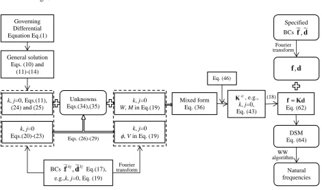
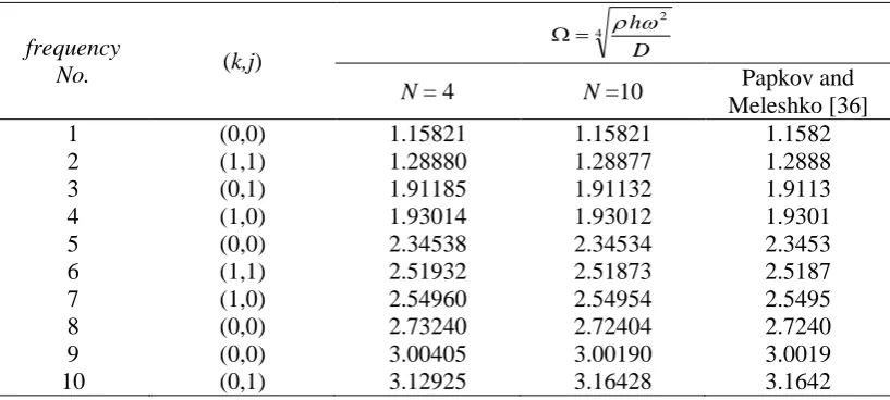
engineering or elastodynamic context. Meleshko [35] and Papkov and Meleshko [36] made ground-breaking
contributions to the study of the free vibration and static bending problems of rectangular plates. This was
achieved by seeking the general solution of the bi-harmonic equation. However, their investigations were
focused on a plate with completely free or completely clamped boundary conditions at all edges, and they did
5
plate has opened up novel, but potential possibilities and has become an important catalyst for the present
research.
As stated earlier, the fundamental basis of the dynamic stiffness formulation for a rectangular plate originates
from the quest for a general solution of the free vibratory motion of the plate represented by the bi-harmonic
equation. This is achieved in this paper in a robust, elegant and exact manner. To this end, the proposed theory
characterises any arbitrary (asymmetric) transverse displacement of the plate in a novel way by using four
sub-solutions of the bi-harmonic equation. Appropriate choices are made for their representations as even and
odd functions so as to include all possible solutions. This is one of the most important steps taken during the
theoretical development. Once the exact solution for the bi-harmonic equation is obtained, the expressions for
bending rotation, shear force and bending moment are formulated. Finally the force displacement relationship
on the plate boundaries is constructed by deriving the frequency dependent dynamic stiffness matrix whilst
eliminating the unknown coefficients from the general solutions of the free vibratory motion. Although the
steps leading to the dynamic stiffness matrix are explained above in a simple manner, the implementation of
these steps is of huge complexity as will be shown later. It should be recognised that the solutions of the
bi-harmonic equation as well as the expressions for transverse displacements, rotations, shear forces and bending
moments are all in series form and the number of terms to be considered in the series to achieve desired
accuracy can be decided in advance and as such there is no limitation in computer implementation of the
theory developed.
2. Theory
2.1. Classical plate theory (CPT) and a general outline of the dynamic stiffness development
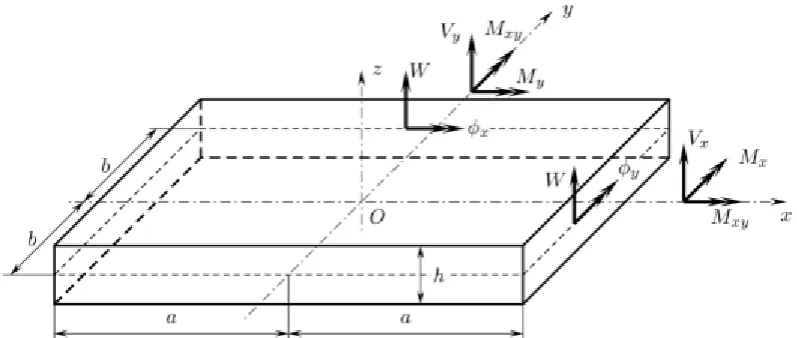
In a right-handed Cartesian coordinate system, Fig. 1 shows a uniform rectangular plate of length 2a, width 2b
and thickness h, respectively. The origin ‘O’ is chosen at the mid-plane and centre of the plate so that the
symmetry of the plate about xy, yz and zx planes is maintained. In the derivation that follows, Kirchhoff’s
thin-plate assumptions [5] are adopted so that the displacement of the mid-plane is uniquely described by the
transverse or flexural displacement w which is a function of the x and y coordinates only, and not of the
6
Fig. 1 Coordinate system and notations for displacements and forces for a thin plate
The governing differential equation of motion of a thin plate, as shown in Fig. 1 undergoing free vibration is
well established in [7, 8] or can be derived using standard texts [16-18]. For harmonic oscillation, i.e. when
t i
e y x W t y x
w( , , ) ( , ) , W being the amplitude of transverse displacement and
the circular (or angular)frequency of oscillation, the differential equation is given by [7, 8]
0
2 4
4 4 2 2 4 4
4
W y
W y
x W x
W
(1)
where 4h2/D is the frequency parameter, DEh3/[12(12)] is the plate bending or flexural rigidity, E
the Young’s modulus, the Poisson ratio and
the density of the plate material.The expressions for the amplitudes of the bending rotations yand
x, the shear forces Vx and Vy and bendingmoments Mx and My per unit length in the usual notation are given by [7, 8]
; y W ;
x W
x
y
(2)
; )
2 ( ;
) 2
( 2
3
3 3
2 3
3 3
y x
W y
W D V y
x W x
W D
Vx y
(3)
;
; 2
2
2 2
2 2
2 2
x W y
W D M y
W x
W D
Mx y
(4)
7
Next, the displacement vector
d
~
comprising the amplitudes of transverse displacements and bending rotationson the four sides of the plate, and the corresponding force vector
~
f
which represents the amplitudes of shearforce and bending moment, are written in the following form
) , (
) , (
) , (
) , (
) , (
) , (
) , (
) , (
~
b x
b x W
y a
y a W
b x
b x W
y a
y a W
x y x y
d
and
) , (
) , (
) , (
) , (
) , (
) , (
) , (
) , (
~
b x M
b x V
y a M
y a V
b x M
b x V
y a M
y a V
y y
x x
y y
x x
f
(5)
It is now necessary to outline broadly the mathematical process of dynamic stiffness formulation to relate the
vectors
d
~
and~
f
of Eq. (5). A general procedure to develop the dynamic stiffness matrix of a structuralelement can be briefly summarized as follows
(i) Seek a closed form general solution of the governing differential equations describing the free
vibratory motion of the structural element in an exact sense in terms of the unknown
coefficients appearing in the general solution.
(ii) Apply general boundary conditions (BCs) in algebraic form for the amplitudes of both
displacements and forces at the boundaries of the element.
(iii) Eliminate the unknown coefficients by relating the amplitudes of the harmonically varying
forces to those of the corresponding displacements and thereby generating the frequency
dependent dynamic stiffness matrix.
As it is well known, the closed form solution for free vibration analysis of a rectangular thin plate has been
widely reported only for the special case when the opposite sides of the plate are simply supported. This is the
so-called Levy solution [7, 8] which simplifies the problem drastically because it reduces the number of
unknown coefficients to just four. However, for the general case when the plate is completely free to deform
in any arbitrary shape, the problem becomes immensely more difficult. Therefore for the general case, it is
necessary to seek the solution of the governing differential equation with sufficiently large number of
unknown coefficients (which ideally extends to infinity) to satisfy any combinations of boundary conditions.
Using the theory presented in this paper, such a solution can be achieved and the results can be accurate even
up to machine accuracy.
2.2. General solution for free vibration of a rectangular plate
8
method of separation of variables allows the general solution of the type
qy px Ce y x
W( , ) (6)
where p and q are wave parameters. Substituting the above equation into Eq. (1) yields the characteristic
equation
2 2 2
q
p (7)
Therefore, any combination of p, q and
satisfying Eq. (7) represents a solution of Eq. (1). Following thework of Gorman [10], an infinite series of base solutions are sought by introducingpn i
n or i
~n in thex direction, where
n0,1,2,...
an
n
and )
1,2,...
2 1 (
~ n n
a
n
depending upon the symmetric or
antisymmetric forms of deformation of the plate which will be explained later. An inspection of Eq. (6)
indicates that the deformation in the x direction can be represented by one symmetric (even) and one
anti-symmetric (odd) harmonic equations, namely
x e
e i
x e
e
n x
i x i
n x
i x i
n n
n n
sin 2
1
cos 2
1
(8)
which applies also for
~
n.Inserting pni
n into Eq. (7) gives2 2 2
n n
q (9)
where the roots of
q
n must appear either in real or in purely imaginary pairs. In the same way, thecorresponding function in y can be separated into symmetric and anti-symmetric pairs as well. A second
infinite series of base solutions can be generated by letting qn i
nor i
~n in the y direction with
n , , ,...
b n
n 01 2
or (n )
n , ,...
b ~
n 1 2
2
1
following an analogous procedure as above. To this end,
the resulting two infinite series of base solutions are added together to form the general solution W of Eq. (1).
The solution can be partitioned into a sum of the four sub-solutions in each of which the function W is either
even or odd. Thus letting
11 10 01 00 1
0 ,
W W W W W W
j k
kj
(10)
9
y. The index ‘0’ denotes an even function whereas ‘1’ denotes an odd function. For example, W00 means W is
even in both x and y whereas W01means W is even in x, but odd in y and so on and so forth. Thus, the four sub-solutions describe the symmetric and anti-symmetric deformations of the plate about the mid-planes. Note
that it follows from the fact that if a structure possesses a plane or planes of symmetry, any asymmetric (or
un-symmetric) motion can be described by the superposition of symmetric and anti-symmetric motions. By
making use of the symmetry of the structure (see Fig. 1) we can construct solution of the differential equation
(1) for each of the four component cases in Eq. (10) as follows
1 2 1 1 2 1 0 0 0 0 00 cos ) cosh cosh ( cos ) cosh cosh ( cosh cos cosh cos n n n n n n n n n n nn p y B p y x C q x D q x y
A x D x C y B y Α W (11)
1 2 1 1 2 1 0 0 01 ~ sin ) ~ cosh ~ cosh ( cos ) sinh sinh ( sinh sin n n n n n n n n n n n n y x q D x q C x y p B y p A y B y Α W (12)
1 2 1 1 2 1 0 0 10 cos ) sinh sinh ( ~ sin ) ~ cosh ~ cosh ( sinh sin n n n n n n n n n n n n y x q D x q C x y p B y p A x D x C W (13)
1 2 1 1 2 1 11 ~ sin ) ~ sinh ~ sinh ( ~ sin ) ~ sinh ~ sinh ( n n n n n n n n n n nn p y B p y x C q x D q x y
A
W
(14) where 2 2 2 2 2 1 2 2 2 2 2 1 2 2 2 2 2 1 2 2 2 2 2 1 ~ ~ ; ~ ~ ; ~ ~ ; ~ ~ ; ; ; n n n n n n n n n n n n n n n n q q p p q q p p (15) with ... , 2 , 1 , / ) 2 / 1 ( ~ ; / ) 2 / 1 (
~ / ; / , 0,1,2,...
n a n b n n a n b n n n n n (16)
and the unknown coefficients An,Bn,Cn,Dn (n =0, 1, 2,…) are different for each of the four component cases
in W. Note that trigonometric and hyperbolic functions in cosine and sine exhibit even and odd characteristics
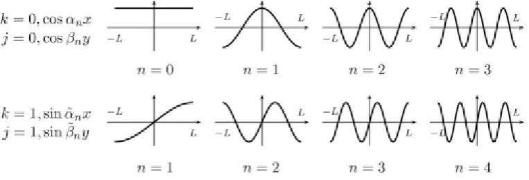
which are exploited here to advantage. The symmetric (k or j=0) and antisymmetric (k or j=1) trigonometric
functions with the first several wavenumbers n,
n and
~n,
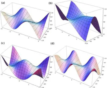
~n taken as in Eq. (16) are depicted in Fig. 2.Due to the properties of orthogonal functions, the general solution composed from Eqs. (11)-(14) can
10
boundaries. It is quite obvious to understand this for transverse displacements because all the trigonometric
functions taking the values of either 1 or 1 on the boundaries at x=±a or y=±b as shown in Fig. 2 where L=a
or b. It can be easily deduced that for any other arbitrary boundary conditions, such as the bending rotations,
bending moments and shear forces defined in Eqs. (2)-(4) can be represented by the set of general solutions by
[image:11.595.108.490.189.319.2]looking at the second- and third-order derivatives of the solutions (11)-(14).
Fig. 2 The first four symmetric/antisymmetric trigonometric functions (L=a or b)
Therefore the general solution given by Eq. (10) when considered as the sum of the sub-solutions given by
Eqs. (11)-(14) satisfies the governing differential equation (see Eq. (1)) a priori. The unknown coefficients
n n n n B C D
A, , , need to satisfy any given boundary conditions of the plate. The fulfilling of boundary conditions
leads to infinite systems of linear algebraic equations relating the Fourier coefficients of the boundary
conditions (both displacements and forces). In the current work, the derived infinite system of linear algebraic
equations is used to develop the dynamic stiffness matrices. We mention in passing that for a plate when all
the edges are either clamped or free, the infinite systems can be solved by using limitants theory [35]. This
particular aspect was investigated by Meleshko [35] and Papkov and Meleshko [36] in recent years.
The displacement and the force vectors in Eq. (5) can now be split into four symmetric and anti-symmetric
components so that the sum of the four sub-vectors in each case represents the net displacement and net force
acting on the boundaries of the plate. In this way one can write
;
) , (
) , (
) , (
) , ( ~
b x
b x W
y a
y a W
kj x
kj kj y
kj
kj
d
) , (
) , (
) , (
) , ( ~
b x M
b x V
y a M
y a V
kj y kj y
kj x kj x
kj
f (k, j = 0, 1) (17)
Now with the help of Eq. (10), the net displacement vector
d
~
and the force vector~
f
of Eq. (5) can be written11 ; ) , ( ) , ( ) , ( ) , ( ) , ( ) , ( ) , ( ) , ( ) , ( ) , ( ) , ( ) , ( ) , ( ) , ( ) , ( ) , ( ) , ( ) , ( ) , ( ) , ( ) , ( ) , ( ) , ( ) , ( ) , ( ) , ( ) , ( ) , ( ) , ( ) , ( ) , ( ) , ( ~ 11 10 01 00 11 10 01 00 11 10 01 00 11 10 01 00 11 10 01 00 11 10 01 00 11 10 01 00 11 10 01 00 b x b x b x b x b x W b x W b x W b x W b x b x b x b x b x W b x W b x W b x W y a y a y a y a y a W y a W y a W y a W y a y a y a y a y a W y a W y a W y a W x x x x x x x x y y y y y y y y d ) , ( ) , ( ) , ( ) , ( ) , ( ) , ( ) , ( ) , ( ) , ( ) , ( ) , ( ) , ( ) , ( ) , ( ) , ( ) , ( ) , ( ) , ( ) , ( ) , ( ) , ( ) , ( ) , ( ) , ( ) , ( ) , ( ) , ( ) , ( ) , ( ) , ( ) , ( ) , ( ~ 11 10 01 00 11 10 01 00 11 10 01 00 11 10 01 00 11 10 01 00 11 10 01 00 11 10 01 00 11 10 01 00 b x M b x M b x M b x M b x V b x V b x V b x V b x M b x M b x M b x M b x V b x V b x V b x V y a M y a M y a M y a M y a V y a V y a V y a V y a M y a M y a M y a M y a V y a V y a V y a V y y y y y y y y y y y y y y y y x x x x x x x x x x x x x x x x f (18)
Once the dependency between sub-vectors
d
~
kj and kjf ~
is determined, which defines the dynamic stiffness
matrix
K
kj for each case arising from the symmetry, it becomes possible with the help of Eq. (18) to derivethe overall dynamic stiffness matrix
K
for the complete plate, which relates the vectorsd
~
and~
f
.2.3. Dynamic stiffness development
In total, four dynamic stiffness (DS) matrices
K
kj should be formulated for four different symmetric andantisymmetric cases. Here for the purposes of illustration, the procedure to develop the DS matrix
K
00 for the component quarter plate representing the symmetry about both the x and the y axes of the whole plate ispresented. The procedure for DS development for the other three cases follows similarly.
The DS matrix
K
00 can be formulated using two steps based on the elimination of the unknown coefficientsin the general solution in Eq. (11), namely,
A
0,
B
0,
C
0,
D
0,
A
n,
B
n,
C
n andD
n . First, the unknowncoefficients
A
0,
B
0,
C
0,
D
0,
A
n,
B
n,
C
n andD
n are obtained by equating the Fourier series of the boundaryconditions for rotations and shear forces to the corresponding expressions obtained from the general solution
and its differentiations. Secondly, the expressions of these unknowns are substituted into the boundary
transverse displacements and bending moments to form an infinite system of algebraic equations which
eventually leads to the DS matrix
K
00.Thus as the first step, it will be shown how the unknowns
A
0,
B
0,
C
0,
D
0,
A
n,
B
n,
C
n andD
n can obtained.12 ; cos cos cos cos ~ 1 1 2 2 1 1 1 1 00 0 0 0 0
n n x x n n n n y y n n x x W W y y W W n n n n
d
1 1 1 1 00 cos cos cos cos ~ 0 0 0 0 n n y y n n y y n n x x n n x x x M M x V V y M M y V V D n n n n
f (19)Alternatively,
~
d
00 and ~f00 can be obtained by evaluating the two-dimensional functions of Eq. (17) (all derived from general solution Eq. (11)) on the plate boundaries. From the general solution for displacement00
W (see Eq. (11)), the bending rotations
y00, 0 0 x
, the shear forces 00 xV , Vy00 and the bending moments
00 00
, y
x M
M can be obtained with the help of Eqs. (2)-(4) and they are expressed as follows:
13 . cos ) cosh ) ( cosh ) ( ( cos ) cosh ) ( cosh ) ( ( cosh cos cosh cos / ) , ( 1 2 2 2 2 1 2 2 1 1 2 2 2 2 1 2 2 1 2 0 2 0 2 0 2 0 00 y x q q D x q q C x y p p B y p p A x D x C y B y A D y x M n n n n n n n n n n n n n n n n n n n n x
(24) . cos ) cosh ) ( cosh ) ( ( cos ) cosh ) ( cosh ) ( ( cosh cos cosh cos / ) , ( 1 2 2 2 2 1 2 2 1 1 2 2 2 2 1 2 2 1 2 0 2 0 2 0 2 0 00 y x q q D x q q C x y p p B y p p A x D x C y B y A D y x M n n n n n n n n n n n n n n n n n n n n y
(25)A close inspection on Eqs (20)-(25) reveals that the expressions with odd order derivatives of W00 (rotation and shear forces) are of simpler forms on the boundaries which can be used to determine all of the unknown
coefficients in terms of the Fourier coefficients of the boundary rotations and shear forces only. For example,
in Eqs. (20) and (22), the terms including sinnx vanish on the boundary at xa since sinna0. Similarly, the conditions sinny0 in Eqs. (21) and (23) on the boundary at yb will be valid. Based on this observation, the following equalities can be obtained by equating Eqs. (20)-(23) on the boundaries to the
corresponding terms of Fourier series in Eq. (19).
, cos cos ) sinh sinh ( sinh sin ) , ( 1 1 2 2 1 1 0 0 00 0
n n y y n n n n n n n n y y y a q q D a q q C a D a C y a n (26)
cos ,cos ) sinh ) ) 2 ( ( sinh ) ) 2 ( ( ( sinh sin ) , ( 1 2 2 2 2 2 1 1 2 2 1 1 3 0 3 0 00 0
n n x x n n n n n n n n n n n n x y V V D y a q q q D a q q q C a D a C D y a V n (27) , cos cos ) sinh sinh ( sinh sin ) , ( 1 1 2 2 1 1 0 0 00 0
n n x x n n n n n n n n x x b p p B b p p A b B b A b x n x
(28)
cos .14
The Eqs. (26) and (27) lead to the following systems of equations
3 0 0 0 0 / sinh sin / sinh sin 0 0 x y V a D a C a D a C (30) n n x n n n n n n n n n n y n n n n n n V a q q q D a q q q C a q q D a q q C 2 2 2 2 2 1 2 2 1 1 2 2 1 1 sinh ) ) 2 ( ( sinh ) ) 2 ( ( sinh sinh (31)
Similarly, Eqs. (28) and (29) yield
3 0 0 0 0 / sinh sin / sinh sin 0 0 y x V b B b A b B b A (32) n n y n n n n n n n n n n x n n n n n n V b p p p B b p p p A b p p B b p p A 2 2 2 2 2 1 2 2 1 1 2 2 1 1 sinh ) ) 2 ( ( sinh ) ) 2 ( ( sinh sinh (33)
The solutions of system of Eqs. (30)-(33) can be written as:
b V
A y x
sin 2 3 2 0 0 0
; b
V
B y x
sinh 2 3 0 2 0 0
; a
V
C x y
sin 2 3 2 0 0 0
; a
V
D x y
sinh 2 3 2 0 0 0
; (34)
a q q q V D a q q q V C b p p p V B b p p p V A n n y n n x n n n y n n x n n n x n n y n n n x n n y n n n n n n n n n 2 2 2 2 2 1 1 1 2 2 2 2 2 2 2 2 2 1 1 1 2 2 2 2 sinh 2 ) ) 2 ( ( ; sinh 2 ) ) 2 ( ( sinh 2 ) ) 2 ( ( ; sinh 2 ) ) 2 ( ( (35)
Thus all unknown coefficients are now expressed by Fourier coefficients for boundary rotations and shear
forces.
In the next step, an infinite system of linear algebraic equation is obtained by substituting the already
determined unknowns
A
0,
B
0,
C
0,
D
0,
A
n,
B
n,
C
n andD
n given by Eqs. (34) and (35) into the boundaryconditions for transverse displacements and bending moments in Eqs. (11), (24) and (25) so that the infinite
system relates the Fourier coefficients of the boundary displacements and forces. The derivations were
complex but carried out both manually as well as by using symbolic computation package Mathematica and
they were checked against each other. The expressions are recorded in Appendices A-C. Then the dynamic
stiffness matrices are formulated from this infinite system by using some further steps of matrix manipulation.
Note that the following matrix reorganisations are applicable only to the doubly-symmetric component case
(k=j=0), but for the remaining three component cases the procedure is analogous. The infinite system of
15
0 V A M φ A
0 φ A W V A
2 1
mix free
mix clamped
(36)
where the sequences of Fourier coefficients for boundary displacements, rotations, bending moments and
shear forces are
T y x y x
T y x y
x
T x y x y
T m
m m
m m m m
m
V
V
V
V
M
M
M
M
W
W
W
W
...}
,
,
...,
,
,
{
...}
,
,
...,
,
,
{
...}
,
,
...,
,
,
{
...}
,
,
...,
,
,
{
0 0
0 0
0 0
0
0 2 1 2
1
V
M
φ
W
(37)
and the frequency dependent elements of the infinite order matrices
A
clamped,
A
free,
A
mix1,
A
mix2 of Eq. (36)can be easily obtained from the system of Eqs. (A.5)-(A.12). The elements are given in explicit algebraic form
in Appendix D.
For a plate with free boundary condition on all sides, one requires MV0 in Eq. (36) which gives
0 φ A
0 φ A W
free mix
1
(38)
Therefore natural frequencies for a plate with all sides free can be obtained from the equation
0 det
det
1
free
free mix
A A
0 A I
(39)
In an analogous way, the natural frequencies for an all-round clamped plate can be obtained by substituting
0
φ
W
in Eq. (36) leading to the following determinant to give the frequency equation0
detAclamped (40)
The displacement sequences Wand
φ
can now be expressed with the help of Eq. (36) as
M P V P φ
M P V P W
22 21
12 11
(41)
where
1 22
2 1 21
1 1
12 2
1 1
11
)
(
;
)
(
)
(
;
)
(
free mix
free
free mix clamped
mix free mix
A
P
A
A
P
A
A
P
A
A
A
A
P
16
This approach is based on the inverse of matrix
(
A
free)
1 and it allows the construction of the inverse of the dynamic stiffness matrix in the following manner
22 21
12 11 1
00
mn mn
mn mn mn
P P
P P
K , (m, n = 1, 2, …) (43)
Here the dynamic stiffness matrix
K
00 relatesf
00 andd
0000 00 00
d
K
f
(44)in which
T
Tφ W d
M V
f00 , , 00 , (45)
The vectors
V
,
M
,
W
,
φ
in Eq. (45) have already been defined earlier in Eq. (37). Clearly thatf
00 andd
00are the Fourier coefficient vectors of the boundary force and displacement vectors ~f00 and
d
~
00 respectively. The accuracy of the dynamic stiffness elements of Eq. (43) will greatly depend on the accuracy of the inverseof the matrix
A
free. This matrix corresponds to quasi-regular operator in space of limited sequences
thatmakes an accurate inverse of the matrix possible on the basis of the method of reduction. The main advantage
of such an approach is the provision of obtaining practically almost exact inverse of the matrix
A
free. Ifelements of the matrix are defined as ( )1{ mn}m,n0 free
z
A (starting index used is 0 for convenience), then the
following matrix equality must be satisfied
O
I
A
A
free(
free)
1
(46)where
I
andO
are respectively the identity matrix and null matrix of the same order asA
free.Equation (46) leads to the following infinite system for each column of matrix
{
z
m,j}
m0 (j = 0, 1, 2 …) as0 1
, 1 2 2 2 2 1 4 1
0
)
1
(
2
)
coth
(cot
j n
j n n n
n
j
j
z
p
p
b
z
b
z
a
a
(47)
1 1
, 2 2 2 2 1 4 1
0
)
1
(
2
)
coth
(cot
j n
j n n n
n
j
j
z
q
q
a
z
b
b
z
a
(48)
m m j m
n
j n n
m n m n
n m
m j
m m m j
m m
z
q
q
b
z
q
q
b
z
5 2 , 2
1
, 1 2 2
2 2 2 1 2
4 2 2 2
5 2 1
2 2 2 1 5
6 ,
2
)
1
(
2
)
1
(
)
)(
(
)
1
(
4
4
)
1
(
17
m m j m
n
j n n
m n m n
m n
m j
m m m j
m m
z
p
p
a
z
p
p
a
z
7
1 2 , 2
1
, 2 2
2 2 2 1 2
4 2 2 2
7 2 0
2 2 2 1 7
6 ,
1 2
)
1
(
2
)
1
(
)
)(
(
)
1
(
4
4
)
1
(
(50)
where m = 0, 1, 2, …, N.
Following the methodology outlined by Meleshko [35] one can now evaluate the coefficients of the system of
Eqs. (47)-(50) by using the following limits
1 3 1 ) )(
( ) 1 ( 4
lim ) )(
( ) 1 ( 4
lim
1
2 2 2 2 1 2
4 2 2 2
7 2
1
2 2 2 2 1 2
4 2 2 2
5 2
n n m n m
m n
m m
n n m n m
n m
m
m b q q a p p
(51)
Clearly the infinite system of Eqs. (47)-(50) is quasi-regular. Thus there exists some number NR such that the
sum of the off-diagonal elements of each row m (m > NR) of the infinite coefficient matrix of the right-hand
side of Eqs. (47)-(50) is less than the corresponding diagonal element which will always have a positive
value. According to the general theory of Kantorovich and Krylov [39], the system of Eqs (47)-(50) will have
unique solution in the space of bounded sequences
for frequencies which are different from naturalfrequencies.
Using the limitants theory which was originally proposed by Koialovich [37] and generalised by Papkov [38],
one can prove that the bounded solution of this system can be described by asymptotic formula (m) as
follows:
2, 2
)
1
(
m j m
j m
bG
z
2, 1 2
)
1
(
m j m
j m
aG
z
(52)
where Gj is some constant and
(0,1) is a root of the following transcendental equation2 cos 3
) 1 )( 1
(
(53)
Based on the knowledge of the asymptotic behavior described by Eq. (52) it is now possible to use the method
of improved reduction [35, 36] for constructing the matrix
(
A
free)
1. For each infinite column of the resultant matrix on the left hand side of Eqs. (47)-(50), one can determine 2N+2 unknowns z0j,z1j,...,z2N,j,z2N1,j(i.e., the first 2N+2 elements of the jth column of matrix
(
A
free)
1) and one asymptotic constant Gj, which leads to the following reduced system with 2N + 3 equations to provide the solutions0 1
2 2 2 1 2 4
1
, 1 2 2 2 2 1 4 1
0
1
)
1
(
2
)
coth
(cot
j N
n n n n
j N
n
j n n n
n
j j
p
p
b
aG
z
p
p
b
z
b
z
a
a
18 1 1 2 2 2 1 2 4 1 2 2 2 2 1 4 1 0
1
1
2
n N n n n jj N n j , n n n n j j
q
q
a
bG
z
q
q
)
(
a
z
)
b
coth
b
(cot
z
a
(55) m m j m Nn n m n m n
n m m j N n j n n m n m n n m m j m m m j m m q q b aG z q q b z q q b z 5 2 , 2 1 2 2 2 2 2 1 2 4 2 2 2 5 2 1 , 1 2 2 2 2 2 1 2 4 2 2 2 5 2 1 2 2 2 1 5 6 , 2 ) 1 ( 2 ) )( ( ) ) 1 (( 4 ) 1 ( ) )( ( ) ) 1 (( 4 4 ) 1 (
(56) m m j m Nn n m n m n
m n m j N n j n n m n m n m n m j m m m j m m p p a bG z p p a z p p a z 7 1 2 , 2 1 2 2 2 2 2 1 2 4 2 2 2 7 2 1 , 2 2 2 2 2 1 2 4 2 2 2 7 2 0 2 2 2 1 7 6 , 1 2 ) 1 ( 2 ) )( ( ) 1 ( 4 ) 1 ( ) )( ( ) 1 ( 4 4 ) 1 (
(57) a z b zG N j N N j N
N j
2 , 1 2 2 , 2 2 ) 1 ( (58)where m = 0, 1, 2,…, N.
Obviously, if a similar system is analysed in terms of the rows of matrix
(
A
free)
1 from Eq. (46), the same results can be obtained. Therefore the solution of the system of Eqs. (47)-(50) enables the inversion of thematrix
A
free with vastly improved accuracy. Furthermore, it should be recognised that the values ofasymptotic formula for all elements have been successfully achieved.
An alternative way to constructe the dynamic stiffness matrix would be to seek expressions for the force
sequences V and
M
instead. This is based on the system of Eqs. (36) to give φ Q W Q M φ Q W Q V 22 21 12 11 (59) where
free mix clamped mix clamped mix mix clamped clampedA
A
A
A
Q
A
A
Q
A
A
Q
A
Q
1 1 2 22 1 2 21 1 1 12 1 11)
(
;
)
(
)
(
;
)
(
(60)The 22 block dynamic stiffness matrix for the symmetric case can thus be represented by
1121 1222 00 mn mn mn mn mn Q Q Q Q
K (m, n =1,2,…) (61)
19
to derive the dynamic stiffness matrix by using Eq. (43).
By using Eq. (43), one can obtain the stiffness matrix
K
00 and similarly,K
kjfor the three other component cases can be formulated. Relevant expressions for the remaining three cases other thanK
00 are recorded inAppendix C. Finally, with the help of Eq. (18), the overall DS matrix
K
of the entire plate can beconstructed from the four component cases
K
kj. Thus, the final DS matrixK
relatingd
andf
is given in the formKd
f
(62)where the vectors
f
andd
are the Fourier coefficient vectors of the arbitrarily prescribed boundary force and displacement vectors ~f andd
~
respectively.It is often instructive to partition the overall dynamics stiffness matrix
K
according to commonly used specified boundary conditions of the plate. Suppose that the displacement vectord
can be partitioned into twosub-vectors
d
a andd
b such that the displacement sub-vectord
b (which corresponds to fb) and the forcesub-vector
f
a (which corresponds tod
a) are known from the prescribed boundary conditions. Then Eq. (62)can be recast in the following form
b a
b a
bb ba
ab aa
f f d d K K
K K
(63)
where T
ba ab K
K . For many practical applications of free vibration analysis,
f
a andd
b are taken as zero vectors. In such cases, Eq. (63) is reduced to0
d
K
aa a
(64)Thus the natural frequencies can be computed through searching for the zeros of the determinant of the above
reduced DS matrix Kaa. Note that the case of a fully clamped plate cannot be accommodated in this
procedure, but the problem for this case can be solved using the determinant of Eq. (40). Any arbitrarily
prescribed mixed boundary conditions such as line and/or point supports on the boundaries can be represented
by the Fourier coefficient vectors
d
andf
through Fourier transforms. In particular, for constraints involvingpoint supports, an alternative approach incorporating Lagrangian multipliers can be used [25]. Application of
such point constraints using Lagrangian multipliers is beyond the scope of the present paper, but provides
scope for future research. Natural frequencies and mode shapes computation follows from an adapted