Effective Lower Bounding Techniques for Pseudo Boolean Optimization

(1)

Effective Lower Bounding Techniques for Pseudo-Boolean Optimization

Vasco M. Manquinho and Jo˜ao Marques-Silva

IST/INESC-ID, Technical University of Lisbon, Portugal

{

vmm,jpms

}

@sat.inesc-id.pt

Abstract

Linear Pseudo-Boolean Optimization (PBO) is a widely used modeling framework in Electronic Design Automa-tion (EDA). Due to signiﬁcant advances in Boolean Sat-isﬁability (SAT), new algorithms for PBO have emerged, which are effective on highly constrained instances. How-ever, these algorithms fail to handle effectively the informa-tion provided by the cost funcinforma-tion of PBO. This paper ad-dresses the integration of lower bound estimation methods with SAT-related techniques in PBO solvers. Moreover, the paper shows that the utilization of lower bound estimates can dramatically improve the overall performance of PBO solvers for most existing benchmarks from EDA.

1. Introduction

Recent advances in Boolean Satisfiability (SAT) have re-sulted in new practical algorithms for solving the Linear Pseudo-Boolean Optimization problem [2, 4, 6]. These al-gorithms perform a linear search on the possible values of the cost function, starting from the highest, at each step re-quiring the next computed solution to have a cost lower than the previous one. If the resulting instance is not sat-isfiable, then the optimal value is given by the last com-puted solution. By incorporating important features from SAT solvers, like non-chronological backtrack-ing in the search tree, conflict-based learnbacktrack-ing mecha-nisms and lazy data structures, these solvers have been able to solve with success several classes of highly con-strained pseudo-boolean instances. However, these solvers also fail to handle effectively the information provided by the cost function, which can be crucial as the experi-mental results in this paper clearly demonstrate. In order to prune the search due to the value of the cost func-tion we propose the use of methods to estimate a lower bound on the value of the cost function. Whenever the lower bound estimation is higher or equal to the best so-lution found so far, we are able to prune the search tree. Moreover, we also establish conditions for backtrack-ing non-chronologically in the search tree when the search

backtracks due to the lower bound estimate. This paper ex-tends [9] by considering alternative lower bounding proce-dures.

The paper is organized as follows. The ﬁrst part con-centrates on describing how different lower bound esti-mation methods can be applied in pseudo-boolean opti-mization problem, focusing on linear-programming relax-ation and Lagrangian relaxrelax-ation. Section 4 proposes tech-niques for obtaining explanations that allow backtracking non-chronologically when the search is bound due to the lower bound estimate. In addition, the paper presents a num-ber of additional techniques that have proved useful in prac-tical PBO solving. Preliminary experimental results are an-alyzed in section 6 for most existing PBO benchmarks for EDA problems. Finally, the paper concludes in section 7.

2. Preliminaries

In a propositional formula, a literall_j denotes either a variablex_j or its complement x¯_j. If a literall_j = x_j and

xj is assigned value 1 orlj = ¯xj andxj is assigned value

0, then the literal is said to be true. Otherwise, the literal is said to be false.

An instancePof a Linear Pseudo-Boolean Optimization problem can be deﬁned as follows,

minimize

j∈Ncj·xj

subject to

j∈Naijlj ≥bi,

xj ∈ {0,1}, aij, bi ∈N+0, i∈M, N ={1, . . . , n}, M ={1, . . . , m}

(1)

wherec_jis a non-negative integer cost associated with vari-ablex_j, j∈Nanda_ijdenote the coefﬁcients of the literals

lj in the set ofmlinear constraints. Every pseudo-boolean formulation can be rewritten such that all coefﬁcientsa_ij and right-hand sideb_ibe non-negative.

(2)

occurs when the value of allaijcoefﬁcients are greater than or equal tob_i.

If every constraint can be interpreted as a propositional clause then P is an instance of thebinate covering prob-lem(BCP). Covering formulations have been the subject of thorough research work that can be found in [5, 9, 15].

Notice that a linear pseudo-boolean optimization prob-lem can also be viewed as a special case of linear integer programming problem. The linear integer programming for-mulation for the constraints can be obtained if we replace literalsx¯_jby1−x_j. In section 3 we will use this latter for-mulation.

3. Pseudo-Boolean Optimization Algorithms

In [3], P. Barth first proposed an approach based on Boolean Satisfiability (SAT) techniques for solving Pseudo-Boolean Optimization (PBO). This approach consists of performing a linear search on the possible values of the cost function, starting from the highest, at each step requiring the next computed solution to have a cost lower than the previ-ous one. If the resulting instance is not satisfiable, then the solution is given by the last recorded solution. The general-ization of recent advances in SAT resulted in new success-ful algorithms [2, 4, 6] for several sets of PBO instances, namely the incorporation of non-chronological backtrack-ing in the search tree, conflict-based learnbacktrack-ing mechanisms and lazy data structures have been applied with success. The SAT-based approach focuses primarily on finding solu-tions for the problem constraints. Therefore, for highly con-strained problems these techniques are very effective. How-ever, these algorithms find it difficult to deal with the infor-mation from the cost function.

Unlike the SAT-based approach, branch-and-bound al-gorithms [5, 8] have proved to be very effective when the instances to be solved are not highly constrained since they are able to prune the search tree earlier due to estimate of the value of the cost function. In branch-and-bound algorithms upper boundson the value of the cost function are identi-ﬁed for each solution to the constraints, andlower bounds on the value of the cost function are estimated considering the current set of variable assignments. For a given instance

P of a pseudo-boolean optimization problem, letP.upper denote the upper bound on the value of the cost function. The search is pruned whenever the lower bound estimation is higher than or equal toP.upper. In this case it is guar-anteed that a better solution cannot be found with the cur-rent variable assignments and therefore the search can be pruned. The algorithms described in [5, 8, 9, 15] for the bi-nate covering problem follow this approach as well as sev-eral gensev-eral integer programming solvers.

For several instances, specially for low constrained in-stances, the tightness of the lower bounding procedure is crucial for the algorithm’s efﬁciency, because with higher

estimates of the lower bound, the search can be pruned ear-lier. Several procedures can be used for lower bound esti-mation, namely the approximation of a maximum indepen-dent set of constraints (MIS) [5, 9], linear-programming re-laxations [8] or Lagrangian rere-laxations [12].

3.1. Linear Programming Relaxations

Although the approximation of a maximum indepen-dent set of constraints (MIS) is the most widely used lower bound procedure for the binate covering problem (a partic-ular case of PBO) [5, 15], linear programming relaxation (LPR) has also been used with success [8] . It is also of-ten the case that the linear programming relaxation bound is higher than the one obtained with the MIS approach. More-over, linear programming relaxations have long been used as a lower bound estimation procedure in branch-and-bound algorithms for solving integer programming problems [11]. The general formulation of the LPR for a pseudo-boolean problem is obtained from (1) as follows:

minimize zlpr=cx

subject to Ax≥b

0≤x≤1 (2)

where vectorcdefines the non-negative integer cost asso-ciated with every decision variable in vectorx. Entries of matrixAdefines the constraint coefficients and vectorbthe right-hand side of every constraint. The solution of (1) is re-ferred to asz_cp∗, whereas the solution of (2) is referred to as

z∗ lpr.

It is well-known that the solutionz_lpr∗ of (2) is a lower bound on the solutionz_cp∗ of (1) [11]. Basically, any solu-tion of (1) is also a feasible solusolu-tion of (2), but the con-verse is not true. Moreover, for a given solution of (2) where

x∈ {0,1}n_{, we necessarily have}_z∗

cp=z∗lpr. Hence, the

re-sult follows. Furthermore, different linear programming al-gorithms can be used for solving (2), some with guaranteed worst-case polynomial run time [11].

3.2. Lagrangian Relaxations

Lagrangian relaxation (LGR) is a widely used method for computing bounds on the optimal value of the cost function from network optimization to nonlinear program-ming [12, 13]. It also known that for some instances, the bound provided by the Lagrangian relaxation method is tighter than the one obtained by the linear programming re-laxation [12]. Therefore, Lagrangian rere-laxation can be used to provide a quick and tight lower bound on the value of the cost function for pseudo-boolean optimization problems.

(3)

incorporate them in the objective function with associated Lagrangian multipliers.

Given a generic linear optimization problem formulated as:

minimize z∗=cx subject to Ax=b

x∈X (3)

we can deﬁne theLagrangian functionL(µ)as:

L(µ) =min{cx+µ(Ax−b) :x∈X} (4) where vector µ deﬁnes the Lagrangian multiplier associ-ated with each constraint. The Lagrangian Bounding Prin-ciple [12] states that for any vectorµof the Lagrangian mul-tipliers, the value ofL(µ)is a lower bound on the optimal solution of the original optimization problem.

In (3) all constraints are formulated as equalities, while in the pseudo-boolean optimization problem (1) we have in-equality constraints. Therefore, in that case the Lagrangian relaxation problem is formulated as:

L∗₌_max{L₍_µ_{) :}_µ_≥₀_} ₍₅₎

whereL∗ is the optimum value of the Lagrangian relax-ation. The most tight lower bound estimate we can obtain using this method is given byL∗.

Before trying to solve the Lagrangian relaxation prob-lem in order to obtainL∗, we must determine the value of

L(µ)for a given value of µ. Notice that by expanding (4) we have:

L(µ) =min{ j∈Ncjxj+

i∈Mµi((

j∈Naijxj)−bi)} L(µ) =min{

j∈N

αjxj− i∈M

µibi}where

αj= (cj+

i∈Mµiaij)

(6)

In order to obtain the value ofL(µ), for a givenµ, we must determine the value of the decision variablesx_jto be able to minimize the expression. Therefore, we must have

xj = 0wheneverαj ≥0andxj= 1whenαj<0.

Literature from nonlinear programming [13] and net-work optimization [12] provide methods to solve (5), namely gradient methods to approximate the value ofL∗. For the results presented in this paper the approach out-line in [12] is used.

4. Bound-based Conﬂicts

Conditions for backtracking non-chronologically due to the lower bound estimate on the value of the cost func-tion ﬁrst proposed in [9] assume that the lower bounding procedure is the MIS approximation. Next, we review the main ideas about pruning the search tree based on the es-timated value of the cost function and describe the condi-tions to apply when using linear-programming relaxation or Lagrangian relaxation as a lower bound estimation proce-dure.

4.1. Backtracking on Bound-based Conﬂicts

A bound conﬂict in an instance of the pseudo-boolean optimization problem (PBO)Parises when the lower bound is equal to or higher than the upper bound. This condition can be written as

P.path+P.lower≥P.upper (7)

whereP.path is the cost of the assignments already made, P.loweris a lower bound estimate on the cost of satisfying the constraints not yet satisﬁed (as given for example us-ing Lagrangian relaxation), andP.upperis the best solution found so far.

In this situation, our approach is to identify a set of as-signments responsible for the bound conﬂict and build a new propositional clause ω_bc such that it prevents those assignments of being repeated during the search process. Whenω_bcis added, a conﬂict analysis procedure must be carried out to determine to which level of the search tree to backtrack to.

A straightforward approach to build ω_bc would be to consider the decision variable assignments from all levels of the search tree, but in that case the resulting backtrack would necessarily be chronological. In [9] it was already shown that the assignments responsible for the bound con-ﬂict might not be associated with all levels of the search tree.

From (7), we can readily conclude that P.path and P.lower are the unique components involved in each bound conflict. Therefore, we will analyze both theP.path andP.lower components in order to establish the assign-ments responsible for a given bound conflict. Our goal is to define two sets of literalsω_ppandω_plcontaining the ex-planation forP.path andP.lower, respectively. Our bound conflict clauseωbc is defined by the set union of the liter-als inω_ppandω_pl.

We start by studyingP.path. Clearly, the variable assign-ments that cause the value ofP.pathto grow are solely those assignments with a value of 1. Hence, we can deﬁneω_pp such that each variable inω_pp has positive cost and is as-signed value 1:

ωpp={l= ¯xj :Cost(xj)>0∧xj= 1} (8)

which basically states that in order to decrease the value of the cost function (i.e.P.path) at least one variable that is as-signed value 1 has instead to be asas-signed value 0.

(4)

4.2. Lower

Bound

Conﬂicts

from

Linear-Programming Relaxation

When using linear-programming relaxations as a lower bound estimation procedure, the value of P.lower is ob-tained according to the formulation described in section 3.1. In order to determine the set of assignments we can deem re-sponsible forP.lower, we must deﬁneSas the set of con-straints withslack1 variables assigned value 0 in the lin-ear program solution. These are the constraints which ac-tually limit the value of P.lower. If the literals that as-sume value 0 in these constraints were to have a different value, some constraints might be satisﬁed and the value of

P.lowerwould be lower. Therefore, we can consider the as-signments to those literals as the responsible forP.lower and deﬁneω_plas:

ωpl={l:l= 0∧l∈ωi∧ωi∈S} (9)

Clearly,ωpldoes not necessarily depend on all decision lev-els in the search tree. Hence, non-chronological backtrack-ing can result from the conﬂict analysis procedure.

4.3. Lower Bound Conﬂicts from Lagrangian

Re-laxation

In order to determine ωpl using the Lagrangian relax-ation lower bound estimrelax-ation procedure as described in sec-tion 3.2, we can follow a similar approach to the one de-scribed for linear-programming relaxation. LetSbe the set of constraints used in obtaining the value ofP.lowerwhose Lagrangian multiplier is different from 0. We can clearly notice from (6) that the constraints with Lagrangian mul-tiplier equal to 0 are irrelevant for computingP.lower. In this case,ω_plcan be determined as formulated in (9).

Another approach to determine ω_pl is to consider the value ofα_j for each assigned variable fromS. If a given variablex_jis assigned value 0 andα_j >0, then by chang-ing its value to 1 we would increase the value ofP.lower. Or if variablex_jis assigned value 1 andα_j<0, if we were to change the value of x_j, P.lower would raise. Hence, these assignments cannot be deemed responsible for the value ofP.lowerand should not be considered inω_pl.

5. Additional Techniques

In this section we describe additional techniques that have proved useful in implementing a branch-and-bound based PBO tool.

When using LPR for computing lower bounds, one can use the information provided by the LP solution for branch-ing purposes. Essentially, branchbranch-ing is restricted to

vari-1 See [13] for a deﬁnition of slack and artiﬁcial variables.

ables for which the LP solution isnotinteger. Of these vari-ables, the one closest to 0.5 is selected. In the case more than one variable has been assigned value 0.5, then the VSIDS heuristic of Chaff is applied [10].

Another additional technique is the generation of a new constraint when a new better solution is found. When this occurs, P.upper is updated, and one can generate a new

constraint:

j∈Ncjxj ≤P.upper−1 (10)

which requires that a new solution must have cost lower that the lowest cost already identiﬁed for a solution. This type of constraint is referred to as a knapsack constraint [11]. Suppose also the existence of a cardinality constraint of the

form:

j∈Kxj ≥U, K⊆N (11)

In this case we can infer a new constraint, that can be added to the set of constraints. LetV be the sum of theUsmallest coefﬁcientscj of variables denoted by setK. Thus we can

conclude:

j∈Kcjxj≥V (12)

As a result, the following constraint can be inferred:

j∈N−Kcjxj≤P.upper−1−V (13)

6. Experimental Results

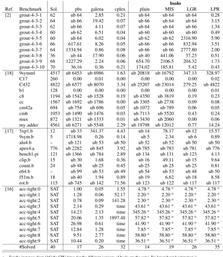
In this section we present empirical results for the tech-niques described in the paper using our pseudo-boolean optimizer (bsolo) which incorporates the branch-and-bound techniques described in the paper and SAT-based techniques, namely boolean constraint propagation, non-chronological backtracking in the search tree and conﬂict-based learning mechanisms.

The CPU times presented are for a AMD Athlon proces-sor at 1.9GHz with 1GB of physical memory. The time limit for each instance was set to one hour. If the time limit was reached, we provide an indication of which was the best up-per bound (ub) value found when the search was stopped.

In order to empirically evaluate the lower bound proce-dures described in the paper, we ran our solver on most PBO instances available, most of which from EDA applica-tions [2, 18, 17, 16]2_{. Besides bsolo, we also ran PBS [2],} Galena [4] and the commercial MILP solver CPLEX (ver-sion 7.5) [1]. For bsolo, we present results when using dif-ferent lower bound methods (MIS, LGR and LPR) and also when no lower bound estimation procedure is used (plain).

The bsolo solver was conﬁgured to use the constraint strengthening technique described in [6] and widely used

(5)

in mixed integer programming [14]. The probing used in the constraint strengthening is also used to detect necessary assignments during preprocessing. We also used simpliﬁca-tion techniques described in [7, 15] in the synthesis bench-mark set.

The results are presented in Table 1. As can be readily concluded, different solvers perform better for different sets of instances. In any case, there are a few clear trends. bsolo (with LPR) is by far the most regular solver, and overall the best performing solver, being able to solve 35 instances out of a total of 40 instances. The other publicly available PBO solvers, PBS and Galena, are solely able to solve 17 and 26 instances, respectively. It should be noted that the general purpose MILP solver CPLEX is extremely compet-itive, being clearly better that both PBS and Galena over all instances. It is also clear that CPLEX is better suited for op-timizing a cost function than for solving a set of pseudo-boolean constraints, as the results for the last benchmarks illustrate.

Despite being a more regular and overall better perform-ing algorithm, bsolo performs worse than both PBS and Galena for the last class of instances [16]. This is essen-tially due to a significantly larger time per decision required by bsolo, motivated by a less optimized implementation of pseudo-boolean constraint propagation. Finally, bsolo with LPR is significantly more efficient than bsolo with LGR. This is motivated by the slow convergence observed for the Lagrangian relaxation on most instances.

7. Conclusions

The paper describes the integration of lower bound es-timation procedures with SAT-based techniques in lin-ear pseudo-boolean optimization, emphasizing two lower bounding methods: linear-programming relaxation and La-grangian relaxation. The paper also outlines a proce-dure for enabling non-chronological backtracking in the search tree when bound conﬂicts occur. In addition, the pa-per proposes a number of additional techniques, includ-ing an informed branchinclud-ing heuristic, and a technique for inferring constraints from knapsack and cardinality con-straints.

Preliminary experimental results, obtained on most of existing PBO benchmarks for EDA problems, are clear: bsolo is the most effective PBO solver, far more effective than either PBS [2] or Galena [4], and is the only dedi-cated PBO solver that is competitive with (and overall sig-niﬁcantly more efﬁcient than) the commercial MILP solver CPLEX [1].

The very promising experimental results clearly demon-strate that the integration of lower bounding techniques is a crucial aspect in the development of PBO solvers, allowing bsolo to be dramatically more efﬁcient than the best pub-licly available PBO solvers, PBS and Galena, which do not

utilize lower bounding techniques. As the experimental re-sults also suggest, the time per decision in bsolo is larger than in either PBS and Galena. This motivates ﬁne-tuning the implementation and data structures of the bsolo proto-type.

References

[1] CPLEX MILP solver. http://www.ilog.com/products/cplex/. [2] F. Aloul, A. Ramani, I. Markov, and K. Sakallah. Generic ILP versus specialized 0-1 ILP: An update. InACM/IEEE International Conference on Computer Aided Design, pages 450–457, November 2002.

[3] P. Barth. A Davis-Putnam Enumeration Algorithm for Lin-ear Pseudo-Boolean Optimization. Technical Report MPI-I-95-2-003, Max Plank Institute for Computer Science, 1995. [4] D. Chai and A. Kuehlmann. A Fast Pseudo-Boolean

Con-straint Solver. InProc. ACM/IEEE Design Automation Con-ference, pages 830–835, 2003.

[5] O. Coudert. On Solving Covering Problems. In Proc. ACM/IEEE Design Automation Conference, pages 197–202, June 1996.

[6] H. Dixon and M. Ginsberg. Inference Methods for a Pseudo-Boolean Satisﬁability Solver. InNational Conference on Ar-tiﬁcial Intelligence, pages 635–640, 2002.

[7] J. Hooker. Logic-Based Methods for Optimization. In . Jon Wiley & Sons, 1996.

[8] S. Liao and S. Devadas. Solving Covering Problems Using LPR-Based Lower Bounds. InProc. ACM/IEEE Design Au-tomation Conference, pages 117–120, 1997.

[9] V. Manquinho and J. Marques-Silva. Search pruning tech-niques in sat-based branch-and-bound algorithms for the bi-nate covering problem. IEEE Transactions on Computer-Aided Design, 21(5):505–516, May 2002.

[10] M. Moskewicz, C. Madigan, Y. Zhao, L. Zhang, and S. Ma-lik. Chaff: Engineering an Efﬁcient SAT Solver. InProc. ACM/IEEE Design Automation Conference, pages 530–535, June 2001.

[11] G. L. Nemhauser and L. A. Wolsey.Integer and Combinato-rial Optimization. John Wiley & Sons, 1988.

[12] T. M. R. Ahuja and J. Orlin. Network Flows: Theory, Algo-rithms, and Applications. Pearson Education, 1993. [13] A. S. S. Nash. Linear and Nonlinear Programming. In .

McGraw-Hill, 1996.

[14] M. Savelsbergh. Preprocessing and probing for mixed inte-ger programming problems. ORSA Journal on Computing, 6:445–454, 1994.

[15] T. Villa, T. Kam, R. K. Brayton, and A. L. Sangiovanni-Vincentelli. Explicit and Implicit Algorithms for Binate Cov-ering Problems.IEEE Transactions on Computer Aided De-sign, vol. 16(7):677–691, July 1997.

[16] J. Walser. 0-1 integer programming bench-marks. http://www.ps.uni-sb.de/∼ walser/benchmarks/-benchmarks.html.

[17] S. Yang. Logic Synthesis and Optimization Benchmarks User Guide. Microelectronics Center of North Carolina, Jan-uary 1991.

(6)

bsolo

Ref. Benchmark Sol. pbs galena cplex plain MIS LGR LPR

[2] grout-4-3-1 62 ub 64 2.85 0.21 ub 64 ub 64 ub 64 0.28

grout-4-3-2 64 ub 66 19.42 0.07 ub 66 ub 64 ub 64 3.15

grout-4-3-3 62 ub 66 4.11 0.07 ub 64 ub 64 ub 66 1.34

grout-4-3-4 60 ub 62 6.51 0.04 ub 60 ub 60 ub 60 0.49

grout-4-3-5 60 ub 64 6.02 0.04 ub 62 ub 62 2316.90 5.90

grout-4-3-6 66 617.61 8.26 0.05 ub 66 ub 66 832.94 3.51

grout-4-3-7 64 1334.94 0.86 0.08 ub 66 ub 66 2777.80 2.00

grout-4-3-8 36 ub 44 17.90 0.06 ub 40 441.06 37.23 0.51

grout-4-3-9 68 1227.29 2.24 0.06 654.70 2106.5 204.32 1.73

grout-4-3-10 70 36.16 0.36 0.21 174.02 185.81 5.42 0.43

[18] 9symml 4517 ub 6453 ub 6986 1.63 ub 20818 ub 16792 347.13 328.97

C17 260 0.00 0.01 0.00 0.00 0.00 0.00 0.02

C432 4822 ub 6577 ub 8070 3.34 ub 25207 ub 23014 279.25 ub 4822

b1 128 0.00 0.00 0.00 0.00 0.00 0.00 0.01

c8 1194 ub 1542 ub 1528 0.19 ub 4350 ub 3819 0.19 0.23

cc 1567 ub 1692 ub 1786 0.00 ub 3305 ub 2738 0.09 0.08

cm42a 694 ub 754 ub 696 0.05 ub 1072 ub 789 0.06 0.05

cmb 1053 ub 1490 ub 1476 0.03 ub 7113 ub 5520 0.43 0.24

mux 872 ub 1321 ub 1333 0.01 ub 3430 ub 2060 0.00 0.06

my adder 4561 ub 6271 ub 5548 2.29 ub 19798 ub 12012 0.77 14.24

[17] 5xp1.b 12 ub 33 341.37 4.43 ub 14 78.17 ub 12 15.57

9sym.b 5 1718.98 0.26 0.14 ub 5 2.34 ub 6 0.89

alu4.b – ub 121 ub 53 ub 50 ub 52 ub 52 ub 50 ub 50

apex4.a 776 ub 2282 ub 845 3.92 ub 785 ub 783 ub 781 ub 776

bench1.pi 121 ub 1366 ub 784 2.89 ub 134 ub 131 ub 123 4.13

clip.b 15 ub 30 1.68 0.36 ub 16 49.11 ub 15 9.64

count.b 24 ub 48 ub 25 0.45 ub 25 ub 25 ub 25 0.81

e64.b – ub 99 ub 53 ub 49 ub 54 ub 53 ub 48 ub 50

f51m.b 18 ub 40 1.94 0.89 ub 19 6.62 ub 18 8.58

rot.b 115 ub 745 ub 142 71.56 ub 123 ub 122 ub 117 ub 117

[16] acc-tight:0 SAT 1.00 0.05 1.55 4.78a _4.78a _4.78a _4.78a

acc-tight:1 SAT 1.28 0.06 52.17 2.20a 2.20a 2.20a 2.20a

acc-tight:3 SAT 2.14 0.29 time 43.61a 43.61a 43.61a 43.61a

#Solved 40 17 26 32 14 19 26 35

[image:6.612.103.557.56.580.2]

a For the instances from [16] the CPU times for the different versions of bsolo are the same. No lower bound estimation is used, since there is no cost function.