Molecular dynamics simulations of mass transfer due to a temperature gradient

Proceedings of CHT-12 ICHMT International Symposium on Advances in Computational Heat Transfer July 1-6, 2012, Bath, England CHT12-CM06

MOLECULAR DYNAMICS SIMULATIONS OF MASS TRANSFER DUE TO A TEMPERATURE GRADIENT

Gülru Babaç*,**,§ , Konstantinos Ritos* and Jason M Reese* *

Department of Mechanical & Aerospace Engineering, University of Strathclyde, Glasgow, UK. **

Institute of Energy, Istanbul Technical University, Istanbul, Turkey. §

Corresponding author. Email: [email protected]

ABSTRACT The molecular dynamics (MD) technique simulates atomistic or molecular interactions and movements directly through Newton’s laws. While to date MD has been mainly applied to study biological systems and chemical processes, there are certain micro and nanoscale engineering applications and technologies that require an understanding of molecular phenomena in order to determine the macroscopic system behaviour. In this paper we demonstrate the application of MD to the benchmark case of the flow of a gas inside a nanochannel connecting two reservoirs with different temperatures. A mass flow is generated between the reservoirs by the thermal gradient — this phenomenon, known as the “Thermal Creep Effect”, is not captured by conventional fluid dynamics with the no-slip boundary condition, and leads to unexpected macroscopic observations. We study the effect of the temperature gradient in cases with different densities and we also report the importance of the wall boundary conditions. Detailed and accurate measurements of temperature, density and pressure that are difficult to obtain through experiments are presented. MD simulations can emulate the realistic molecular conditions and flows, and yield new insight into diffusive transport in non-equilibrium gas flows. This paper demonstrates that the engineer interested in studying and designing new nanotechnologies can deploy molecular dynamics as an effective flow simulation tool.

NOMENCLATURE

N_f[], number of total degrees of freedom

R_cut[m], cut-off distance of the interaction potential

R_ij[m], the distance between molecules i and j

[J], the depth of the intermolecular potential well

[m],the finite distance at which the intermolecular potential is zero

INTRODUCTION

studies have focused mainly in water/solid interactions [e.g.,Werder et al. 2003, Cruz-Chu and Shulten 2006, Hirvi and Pakkanen 2006, Lundgren, Schneemilch and Quirke 2007] and, more recently on water flows through carbon nanotube membranes [e.g.,Corry 2008, Joseph and Aluru 2008, Thomas, McGaughey and Kuter-Arnebeck 2010, Nicholls et al. 2012]. They have also contributed to measuring the probability distribution function of monatomic gases [e.g.,Dongari, Zhang and Reese 2011].

In this paper we demonstrate the application of MD to the benchmark case of the flow of a gas inside a nanochannel that connects two reservoirs with different temperatures, as shown in Figure 1 [e.g., Babac and Sisman 2010]. It is well known that the transport properties of gases at the micro/nano scale differ from those at the macro scale. The Knudsen number (Kn), which is the ratio of the molecular mean free path (λ) to a characteristic length (L) of the flow system, helps categorise gas flows in different regimes, such as continuum, slip flow, transition, and free molecular [e.g., Karniadakis, Beskok and Aluru 2005]. For nano channels, the characteristic flow length is often much smaller than the mean free path of the molecules. Under these conditions, and with Knudsen numbers greater than 10, the gases display non-standard fluid behaviour, and flow properties are determined in the free molecular flow regime.

In the system we investigate, a mass flow is generated between the reservoirs by the thermal gradient — this phenomenon, known as the “Thermal Creep Effect” [e.g., Sone 1991, Sone 2000], is not captured by conventional fluid dynamics with the no-slip boundary condition. This effect results in a temperature gradient-driven “pump”, known as a Knudsen pump [e.g., Knudsen 1910a, Knudsen 1910b, Copic and McNamara 2009]. At steady state in this benchmark case, there is zero net mass flux, and the Knudsen law for Maxwellian gases holds [e.g., Reif 1965], and the density variation along the channel can be predicted with the use of the ideal gas law, such that

pHOT THOT

 pCOLD TCOLD

(1)









1/2

(2)

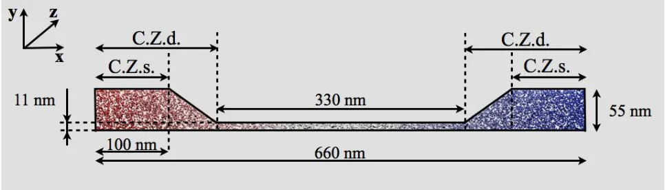
Figure 1. Schematic of the simulated flow system. The depth is uniform all over the system and equal to 22nm. Helium atoms are coloured according to temperature, with red denoting high temperature and blue low temperature. The thermostat is applied within the control zone (C.Z.), which is different for the specular (s) wall and the diffusive (d) wall cases.

METHODS

In this section we present the methodology that has been followed during the numerical simulations. All the necessary parameters for the repetition of the MD simulations are given.

Initialising and Controlling We present results from two configurations with different numbers of molecules. In the first case we have 8000 helium gas atoms inside the system, while in the second one we have 2000. The first case runs in parallel on 16 cores for 29 days, while the second smaller case runs in serial for 10 days. Although the density in the reservoirs differs between the different configurations, they both lead to the same density inside the nano channel at steady state:

0.15kg/m3_.

Given the density and the dimensions of the nano channel we can also calculate the Knudsen number, which is Kn18.5 for all the presented cases. Helium atoms interact with each other through a Lennard-Jones (LJ) potential:



E_P 4 

Rij       12   R_ij         6       

 (3)

For helium-helium interactions we used the known values of



_HeHe 1.96541022_J

and



_HeHe 2.20231010_m

[e.g., Bird, Stewart and Lightfoot 2006]. The potential is truncated and shifted at a distance



R_cut 6.61010_m

in order to improve the computational speed of the MD simulation, without affecting the accuracy significantly. A timestep of 1.3 fs is applied as the high velocities in the initial part of the simulation, see Figure 6, could cause stability problems.

The application of a Berendsen thermostat [e.g., Frenkel and Smit 2001] in the reservoir zones ensures that the temperature remains constant at the target values. For the case with the specular wall boundary condition and the 8000 gas atoms



T_HOT 565.41.4K and



T_COLD290.20.9K, for the

hot and cold reservoirs respectively. These values are



T_HOT 573.30.2K and



T_COLD 287.30.3K for the diffusive wall boundary condition and 8000 gas atoms, and



T_HOT 574.50.4K and



Wall Boundary Conditions In both the x- and y-directions two different types of walls have been modelled: specular and diffusive with linear temperature gradient, while the z-direction is periodic for all cases. In specular wall boundary conditions, when a molecule passes the boundary, the velocity component perpendicular to the wall is reversed and the molecule is reinserted into the computational domain. This method is easily implemented, and substituting a fully atomistic representation with frozen atom walls results in a significant reduced computational cost. However, it is not recommended for non-isothermal flows or when heat transfer between the fluid and the solid wall is important. In our benchmark case this boundary condition affects the shape of the temperature, pressure and density profiles along the system, although it does not significantly affect the absolute values at steady state.

Diffusive wall boundary conditions can be an accurate, and much less computationally intensive, alternative to fully atomistic flexible walls. In our benchmark case we apply diffusive walls with a linear temperature gradient along them. This type of boundary condition has the advantage that heat is transferred from the wall to the gas and provides a more accurate representation of our system. When a gas atom passes the boundary it is reinserted back into the simulation domain with a velocity sampled from the equilibrium Maxwell-Boltzmann distribution at the temperature of the wall. Moreover, the direction of the velocity vector is chosen randomly from a Gaussian distribution. This type of boundary condition has been extensively applied in other methods, such as the direct simulation Monte Carlo (DSMC) method, and its accuracy has been thoroughly studied [e.g., Tysanner and Garcia 2004].

Measurement Techniques Temperature, pressure and density measurements are necessary to characterise the thermodynamic state of the fluid. In MD simulations the momentum of every atom is known and can be measured at every time step. In combination with kinetic theory, we can then calculate the temperature in a simulated system or in parts of it. In practice, we measure the total kinetic energy of the system, divide it by the total number of degrees of freedom and as a result we get the instantaneous temperature.

T  Miui kNf i1

N



Where M_i,u_i,k and N_f are the molecular mass, molecular velocity, Boltzmann constant and number of total degrees of freedom respectively. In cases where we are interested to capture the spatial variation of temperature, or any other physical quantity, we make use of the method of bins. For example, we divide our system into small “bins”, with an average width of 0.66 nm, and then we apply the previously described method of calculating the temperature in each one of them. This allows us to measure the temperature difference between the two reservoirs and also capture and visualise the temperature gradient.

The calculation of pressure is more complex and invokes the virial theorem. The treatment of intermolecular interactions could also involve further correction terms in our calculations.

pkT  1

3V F R

 

16 3  2 2 3 1 R_cut     9  1 R_cut     3         ji

N



i N



p 1

V Miui

2_1

3 jiF R

 





Where V is the system’s volume, is the density of the gas, F R

 

of the interaction potential. In eq. 5 we include the standard kinetic and virial terms for the pressure calculation and also the tail correction when Lennard-Jones interactions are involved, as in our case. However this last term is negligible for gases, and pressure measurements will not significantly change if it is not included in the calculations. With the application of the method of bins, pressure differences between the reservoirs, and the pressure gradient along the nano channel, can be presented.

Finally, we performed number and mass density calculations, although these are constant over the whole system, local variations are possible. Applying the method of bins to the density calculation reveals the change of density along the nano channel and between the two reservoirs:

 1 V i Mi

N



Further measurements can be extracted from a MD simulation, such as thermal conductivity, diffusivity, viscosity, and electrical conductivity. In our benchmark case the only additional property that could give some further insight is the velocity and the velocity profile. Unfortunately, the flow velocities due to the temperature gradient are much lower than the thermal velocity of the gas. As a result, velocity measurements contain a great deal of noise, as will be seen in our results where we averaged over million of samples.

RESULTS AND DISCUSSION

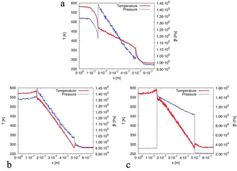
The results from our simulations presented in Figures 2, 3 and 5 have been averaged over 70 ns of simulation time, after reaching the steady state condition, see Figure 4. In Figure 2 the temperature remains almost constant inside the reservoirs, as it is controlled in these areas. Independent of the wall boundary conditions, the temperature drop along the nano channel is then linear, while a steep difference can be observed at the inlet and outlet of the nano channel. When specular boundary conditions are used, the controlled volume is smaller, and the greatest temperature drops occur at the converging and diverging parts of the system.

Figure 2. Temperature and pressure profiles along the simulated system, for different wall boundary conditions and number of atoms. Values are averaged over a simulation time of 90 ns. a) Specular wall boundary conditions and 8000 helium atoms. b) Diffusive wall boundaries, linear temperature gradient along the nanochannel and 8000 helium atoms. c) Diffusive wall boundaries, linear temperature gradient along the nanochannel and 2000 helium atoms.

Moreover, we can apply the Knudsen law, eq. 1, and further verify the existence of the thermal creep effect in all the simulated cases. Substituting the temperature and pressure values from Figure 2.a into eq. 1 we obtain



p_HOT T_COLD p_COLD T_{HOT S} 

1.31105 ₂₉₀

1.0105 ₅₆₅ 0.939 (7)

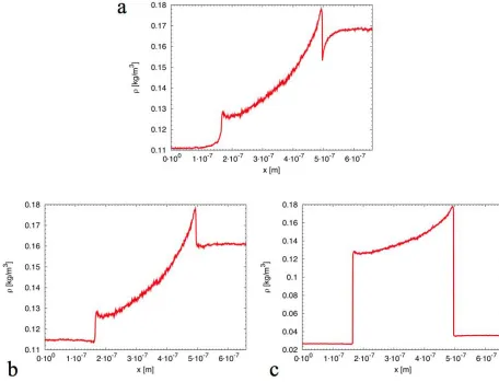
Figure 3. Density profiles along the simulated system, for different wall boundary conditions and number of atoms. Values are averaged over a simulation time of 90 ns. a) Specular wall boundary conditions and 8000 helium atoms. b) Diffusive wall boundaries, linear temperature gradient along the nanochannel and 8000 helium atoms. c) Diffusive wall boundaries, linear temperature gradient along the nanochannel and 2000 helium atoms.

Density profiles along the simulated systems are given in Figure 3. These can be used to show the existence of thermal creep through eq. 2. Again the simulations generally agree with theory in the range between 0.5% and 5%, depending on the boundary condition and number of molecules. The steep jumps in the density profiles reveal the effect of the thermostat in the reservoir zones, and are enhanced as the number density becomes smaller.

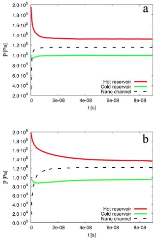
Figure 4. Averaged pressure evolution inside the reservoirs and the nano channel, for a) specular wall and b) diffusive wall case.

Figure 5. Cross-channel fluid velocity profile averaged over the whole length of the nano channel and over 90 ns of simulation time.

Figure 6. Time evolution of the x-component of velocity along the simulated channel.

differences could be simulated in order to capture the actual velocity profile of the thermal creep flow.

ACKNOWLEDGEMENTS

The calculations were performed on the 1100 core HPC facility of the Faculty of Engineering at the University of Strathclyde. The authors would like to thank Matthew Borg of the University of Strathclyde for help with the MD methodology. GB would like to thank the Scientific and Technological Research Council of Turkey (TUBITAK). KR and JMR thank the UK’s Engineering and Physical Sciences Research Council for financial support through grant EP/I011927/1.

REFERENCES

Babac, G. and Sisman, A. [2010], Classical Thermosize Effects and Thermodynamic Cycles, Journal of Computational and Theoretical Nanoscience, Vol. 8, No. 9, pp 1720-1726.

Bird, R. B., Stewart W. E. and Lightfoot, E. N. [2006], Transport Phenomena. Revised 2nd Edition,

John Wiley & Sons, West Sussex

Borg, M. K., Macpherson, G. B., and Reese, J. M. [2010], Controllers for imposing continuum-to-molecular boundary conditions in arbitrary fluid flow geometries, Molecular Simulation, Vol. 36, No. 10, pp 745-757.

Copic, D. and McNamara, S. [2009], Efficiency derivation for the Knudsen pump with and without thermal losses, Journal of Vacuum Science & Technology A, Vol. 27, No. 3.

Corry, B. [2008], Designing carbon nanotube membranes for efficient water desalination, Journal of Physical Chemistry B, Vol.112, No. 5, pp 1427-1434.

Cruz-Chu, E. R. and Shulten, K. [2006], Water-silica force field for simulating nanodevices, Journal of Physical Chemistry B, Vol. 110, pp 21497-21508.

Dongari, N., Zhang Y. and Reese, M. J. [2011], Molecular free path distribution in rarefied gases,

Journal of Physics D, Vol. 44, pp 125502

Frenkel, D. and Smit, B. [2001], Understanding Molecular Simulation: From Algorithms to Applications, Academic Press, London.

Hirvi, J. T. and Pakkanen, T. A. [2006], Molecular dynamics simulations of water droplets on polymer surfaces, The Journal of Chemical Physics, Vol. 125, pp144712.

Joseph, S. and Aluru, N.R. [2008]. Why are carbon nanotubes fast transporters of water?, Nano Letters, Vol. 8, No 2, pp 452-458.

Karniadakis, G., Beskok, A. and Aluru, N. [2005], Microflow and Nanoflows: Fundamentals and Simulation, Springer Science+Business Media, New York.

Knudsen M. [1910a], Eine Revision der Gleichgewichtsbedingung der Gase. Thermische Molekularströmung, Annals of Physics, Vol. 31, pp 205-229.

Lundgren, M., Allan, N. L. and Cosgrove, T. [2003], A molecular dynamics of study of wetting of a pillar-surface, Langmuir, Vol. 19, pp 7127-7129.

Macpherson, G. B., Nordin, N., and Weller, H. G. [2009], Particle tracking in unstructured, arbitrary polyhedral meshes for use in CFD and molecular dynamics, Communications in Numerical Methods in Engineering, Vol. 25, No. 3, pp 263-273.

Macpherson, G. B. and Reese, J. M. [2008], Molecular dynamics in arbitrary geometries: parallel evaluation of pair forces, Molecular Simulation, Vol. 34, No. 1, pp 97-115.

Nicholls, W. D., Borg, M. K., Lockerby, D. A. and Reese, J. M. [2012], Water transport through (7,7) carbon nanotubes of different lengths using molecular dynamics, Microfluidic Nanofluidic, Vol. 12, pp 257-264.

Rapaport, D. C. [2004], The Art of Molecular Dynamics Simulation, CUP, 2nd Ed.

Reif, F. [1965], Fundamentals of Statistical and Thermal Physics, McGraw-Hill, New York.

Schneemilch, M. and Quirke, N. J. [2007], Effect of oxidation on the wettability of poly(dimethylsiloxane) surfaces, The Journal of Chemical Physics, Vol. 127, pp 114701.

Thomas, J.A., McGaughey, A.J.H. and Kuter-Arnebeck, O. [2010], Pressure-driven water flow through carbon nanotubes: insights from molecular dynamics simulation, International Journal of Thermal Sciences, Vol. 49, No. 2, pp 281-289.

Tysanner, M. and Garcia, A [2004]. Measurement bias of fluid velocity in molecular simulations,

Journal of Computational Physics, Vol. 196, pp173-183.

Sone, Y. [1991], A simple demonstration of a rarefied gas flow induced over a plane wall with a temperature gradient, Physics of Fluids A, Vol. 3, No. 5, pp 997-999.

Sone, Y. [2000], Flows induced by temperature fields in a rarefied gas and their ghost effect on the behavior of a gas in the continuum limit, Annual Review of Fluid Mechanics, Vol. 32, pp 779-811.

Werder, T., Walther, J. H., Jaffe, R. L., Halicioglu, T. and Koumoutsakos, P. [2003], On the water-carbon interaction for use in molecular dynamics simulations of graphite and water-carbon Nanotubes,