Influence of vertical flows in wells on groundwater sampling

In

fl

uence of vertical

fl

ows in wells on groundwater sampling

Lindsay A. McMillan

⁎, Michael O. Rivett

, John H. Tellam

, Peter Dumble

, Helen Sharp

Water Sciences Group, School of Geography, Earth & Environmental Sciences, University of Birmingham, Birmingham B15 2TT, UK b

In-Situ Europe Ltd, Stratford Road Shirley, Solihull, West Midlands B90 3AU, UK c

Environment Agency, The Lateral 8 City Walk, Leeds, West Yorkshire LS11 9AT, UK

a r t i c l e i n f o

a b s t r a c t

Article history:

Received 16 December 2013 Received in revised form 8 May 2014 Accepted 16 May 2014

Available online 22 May 2014

Pumped groundwater sampling evaluations often assume that horizontal head gradients predominate and the sample comprises an average of water quality variation over the well screen interval weighted towards contributing zones of higher hydraulic conductivity (a permeability-weighted sample). However, the pumping rate used during sampling may not always be sufficient to overcome vertical flows in wells driven by ambient vertical head gradients. Such flows are reported in wells with screens between 3 and 10 m in length where lower pumping rates are more likely to be used during sampling. Here, numerical flow and particle transport modeling is used to provide insight into the origin of samples under ambient vertical head gradients and under a range of pumping rates. When vertical gradients are present, sample provenance is sensitive to pump intake position, pumping rate and pumping duration. The sample may not be drawn from the whole screen interval even with extended pumping times. Sample bias is present even when the ambient vertical flow in the wellbore is less than the pumping rate. Knowledge of the maximum ambient vertical flow in the well does, however, allow estimation of the pumping rate that will yield a permeability-weighted sample. This rate may be much greater than that recommended for low-flow sampling. In practice at monitored sites, the sampling bias introduced by ambient vertical flows in wells may often be unrecognized or underestimated when drawing conclusions from sampling results. It follows that care should be taken in the interpretation of sampling data if supporting flow investigations have not been undertaken.

© 2014 The Authors. Published by Elsevier B.V. This is an open access article under the CC BY license (http://creativecommons.org/licenses/by/3.0/). Keywords:

Groundwater monitoring Permeability-weighted samples Monitoring wells

Well purging Ambient vertical flows Low-flow sampling

1. Introduction

Groundwater quality observed from the sampling of monitoring wells (or boreholes) is fundamentally controlled by the origin of the groundwater extracted. Sample prove-nance may depend upon a complex interplay of the scale (e.g. screen length) of the monitoring well, the sampling method and protocol employed and the prevailing local hydrogeological conditions. The latter's influence may prove

to be significant between wells even where similar sampling protocols are adopted that are designed to promote consis-tency in approaches. Variation in the local permeability field (and hence natural groundwater flow regime) may cause traditional well purging approaches advocating remov-al of three to five or more well volumes (ASTM International, 2013) to exhibit contrasting interactions with the various (hydro)geological units present. Likewise, increasingly adopted, passive zero-purge or low-flow (0.1–0.5 l/min) sampling methods (Puls and Barcelona, 1996), may extract samples significantly influenced by the natural groundwater flow regime that is sensitive to local hydrogeological scenario (and the well's potential perturbation of that regime). Zero purge or low-flow sampling might not always be recom-mended (US EPA, 2010), but are nevertheless often attractive ⁎ Corresponding author at: School of Geography, Earth & Environmental

Sciences, University of Birmingham, Birmingham B15 2TT, UK. Tel.: +44 121 414 6165.

E-mail address:[email protected](L.A. McMillan).

1_{Now at: Peter Dumble Hydrogeology, Tiverton, Devon EX16 7TA, UK.}

http://dx.doi.org/10.1016/j.jconhyd.2014.05.005

0169-7722/© 2014 The Authors. Published by Elsevier B.V. This is an open access article under the CC BY license (http://creativecommons.org/licenses/by/3.0/). Contents lists available atScienceDirect

Journal of Contaminant Hydrology

compared to onerous well purging due to their potential benefits of reducing purge volume, minimizing in-well disturbance, reducing mixing with casing water, and short-ened sampling times (Barcelona et al., 1994, 2005; Puls and Barcelona, 1996; Stone, 1997). It is hence important that potential influences of the local hydrogeological flow regime upon groundwater samples withdrawn by both modern and established sampling protocols are rigorously assessed to allow more appropriate sampling of wells and interpretation of the groundwater quality data arising.

While the influence of the local permeability field on sample origin is widely recognized through the concept that pumped samples are permeability weighted (i.e., higher permeability layers contribute a greater proportion to the sample obtained (Church and Granato, 1996; Hutchins and Acree, 2000; Puls and Barcelona, 1996)), consideration of local hydraulic, particularly vertical gradients, is often neglected. Critically, the monitoring well may serve as an artificial conduit allowing vertical flows between otherwise unconnected geological units. This can result in unforeseen sample origins that may remain unrecognized in the absence of supporting flow or gradient data. Our primary interest herein is to evaluate the influence of vertical flows in wells on the provenance of the pumped sample and groundwater quality determined.

Our research adds to that undertaken on the provenance of pumped samples from wells. At long time, pump intake position may not be important and the sample origin is directly related to the permeability distribution over the well screen interval (Varlijen et al., 2006). However, it may take a significant time, often longer than the typical sampling time, before this permeability-weighted sample concentration is attained due to the later arrival of groundwater entering the distant ends of the screen farthest from the pump intake (Martin-Hayden, 2000a,b; Martin-Hayden et al., 2014; Reilly and Gibs, 1993). Well casing storage (Barber and Davis, 1987), well screen and sand pack design (Kozuskanich et al., 2012), the partial mixing of inflowing water with water within the well screen during pumping (Martin-Hayden and Wolfe, 2000) and even the purging method (Robbins and Martin-Hayden, 1991) may additionally affect the stabiliza-tion time. With increasing screen length in particular, chemical stability may take a very long time to occur, even if pumping rates are increased (Mayo, 2010; Rivett et al., 1990).

Implicit to many groundwater sampling evaluations is the (perhaps unrecognized) assumption that pumping overcomes any ambient vertical gradients and a permeability-weighted sample (also referred to as a flow-weighted average sample or a screen-weighted sample (Church and Granato, 1996; Hutchins and Acree, 2000; Martin-Hayden, 2000a)) is eventu-ally obtained. However, rather than being the exception (Giddings, 1987), ambient vertical flows in wells are expected to be as ubiquitous as vertical flows in aquifers and will occur at least to some degree in all aquifers (Elci et al., 2001). Naturally occurring vertical hydraulic head gradients which may induce significant vertical flows in wells are widely reported in a variety of hydrogeological settings (Brassington, 1992; Church and Granato, 1996; Dumble et al., 2006; Furlong et al., 2011; Ma et al., 2011; Metcalf and Robbins, 2007; Streetly et al., 2002; Taylor et al., 2006). Ambient vertical flows

in wells are likely to be greater where well screens are longer and geological layering promotes increased vertical head gradients. Use of shorter screens (low-flow sampling is typically recommended for well screensb3 m (e.g.US EPA, 2010)) may reduce ambient vertical flows, however, ambient vertical flows of 0.015–2.3 l/min have been reported in wells with screens between 3 m and 10 m in length (Elci et al., 2001). It is important to recognize the influence of vertical flows in wells as they may cause aquifer cross-contamination (Lacombe et al., 1995), passive sample concentration bias (Elci et al., 2001; Konikow and Hornberger, 2006), errors in hydraulic head and hydraulic conductivity estimation (Elci et al., 2003; Kaleris et al., 1995) and misinterpretation of tracer test results (Riley et al., 2011). The effect and sensitivities of ambient vertical flows on sampling provenance in pumped groundwater samples has not been systematically mapped out.

Our goal is hence to examine the phenomenon of ambient-flow biased samples and answer the question— can the literature-reported range of vertical flows in wells bias sampling results and lead to samples that are weighted by ambient head gradients in addition to other hydraulic influences? We present herein our numerical modeling study designed to address this question.

2. Materials and methods

2.1. Numerical modeling overview

Numerical flow modeling with particle tracking was used to investigate pumped sample provenance under ambient hori-zontal head gradients and for increasing vertical gradients for 14 different model scenarios with varying screen lengths, well diameters, pumping rates, aquifer depths, permeability distri-butions and boundary conditions (Table 1). For each scenario the relative influence of vertical head gradients was varied by varying the position of the monitoring well in the aquifer. Each vertical flow simulation was compared with a corresponding baseline case with the same scenario parameters but no ambient vertical head gradients.

water tables. Also long well screens may be found in older wells/boreholes inherited from long-term monitoring of aquifer resources or, for example, sentinel monitoring at landfill sites where a reasonable thickness of a potentially impacted aquifer may be monitored.

Vertical flow simulations for each scenario were run initially without pumping to assess the induced ambient vertical flows in the well. Pumping at low-flow rates was then simulated to investigate the sampling bias induced by the aquifer vertical gradients. Finally for each scenario, the pumping rate was increased to see if vertical gradients could be overcome and permeability-weighted sampling conditions could be achieved. Several transient simulations were used to investigate the possible variation in flux distribution as drawdown proceeds;

in particular, the arrival at the pump intake of water initially in the casing.

The scope of the modeling excluded direct assessment of the implications of water quality variations within a monitored aquifer. The modeling results will assume more importance where concentration variations are significant between different geological (permeability) horizons sam-pled by the well. Our flow-based assessment underpins such future work.

2.2. Model setup

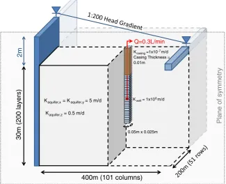
MODFLOW 2000 (Harbaugh et al., 2000) was used to model the sampling scenarios simulated (Fig. 1). The model's

Q=0.3L/min

0.05m x 0.025m

30m (200 layers)

Plane of symmetry

Kaquifer,x= Kaquifer,y= 5 m/d

Kaquifer,z= 0.5 m/d

400m (101 columns)

Kcasing=1x10-7m/d

Casing Thickness = 0.01m

Kwell= 1x106m/d

2m

Fig. 1.Summary of model domain and parameters for Scenario 1 with vertical head gradients (not to scale).

Table 1

Summary of model parameters for 14 scenarios. Scenario Screen

length (m) Well diameter (cm)

Kx,y (m/day)

Anisotropy ratio (Kv:Kh)

Kx,y,z(m/day) (LowKlayer)

Screen K (m/day)

Aquifer depth (m)

Boundary Pump rate (l/min)

1 6 5 5 1:10 N/A N/A 30 C.H. 0.3

2 6 5 5 1:1 N/A N/A 30 C.H. 0.3

3 6 5 0.5 1:10 N/A N/A 30 C.H. 0.3

4 6 5 0.5 (top 50%) 5 (bottom 50%) 1:10 N/A N/A 30 C.H. 0.3

5 6 10 5 1:10 N/A N/A 30 C.H. 0.3

6 6 5 5 1:10 N/A 0.5 30 C.H. 0.3

7 6 5 5 1:10 N/A 0.05 30 C.H. 0.3

8 3 5 5 1:10 N/A N/A 30 C.H. 0.3

9 10 5 5 1:10 N/A N/A 30 C.H. 0.3

10 6 5 5 1:10 N/A N/A 60 C.H. 0.3

11 6 5 5 1:1 0.05 (middle) N/A 30 C.H. 0.3

12 6 5 5 1:1 0.05 (top) N/A 30 C.H. 0.3

13 6 5 5 1:10 N/A N/A 30 Recharge 0.3

finite difference grid was 400 m wide and either 30 or 60 m deep. Variable horizontal grid spacing was used ranging from a minimum as dictated by the borehole diameter to a maximum of 30 m at the inflow boundary. Uniform vertical discretization was used. The existence of a vertical plane of symmetry through the borehole and parallel to groundwater flow allowed half the domain of interest to be simulated.

Head boundaries were specified at the left- and right-hand sides of the model. The remaining boundaries were no flow. For baseline no ambient vertical flow simulations the head gradient between left and right boundaries was uniform with depth in the aquifer. In these simulations, the well was centered both vertically and horizontally in the aquifer. For vertical flow cases, the conceptual model was one of predominantly horizontal regional flow from an aquifer discharging at a surface-water body with vertical gradients increasing as discharging water converges at the outflow point. For these scenarios, the right constant head boundary was specified in the top layer of the model only.

Rather than fixing well inflows/outflows or near well hydraulic gradients, for vertical flow simulations model bound-ary conditions were specified at a distance from the well. This allowed pumping simulations to affect (and possibly overcome) near well vertical head gradients. For each scenario the influence of vertical gradients on the well was varied by varying the horizontal distance of the well from the outflow boundary.

Initial sensitivity testing demonstrated that increasing the horizontal head gradient between the inflow and outflow boundaries leads to increased vertical head gradients due to the larger volume of water converging on the outflow point. Therefore, the horizontal gradient acted as a control on the magnitude of any in-well vertical flows. A final horizontal hydraulic head gradient of 1:200 was chosen as being both a realistic value, and one able to generate ambient vertical well flow rates that were comparable to those reported in literature.

While possibly important during groundwater sampling at some sites, variation in sample origin due to well dewatering effects was out with the scope of this investigation. In order to prevent well dewatering effects in the unconfined simulations, the model head gradients were specified such that they were above the top boundary of the model. The only exception to this was Scenario 13 where model inflows were derived from recharge alone with no left-hand constant head boundary. In this scenario, recharge was uniformly distributed at a rate of 1.41 mm/day. The recharge value was selected to give model inflows comparable to Scenario 1.

It was hypothesized that any impedance to vertical flow in the aquifer was likely to be important in driving ambient vertical well flows. For this reason, the starting vertical scenario (scenario 1) was that of a permeable (5 m/day) aquifer with a 1:10 vertical to horizontal anisotropy ratio. Aquifer hydraulic properties in subsequent scenarios were chosen to represent a non-exhaustive range of alternatives: an isotropic aquifer (Scenario 2); a lower permeability aquifer (Scenario 3); a two-layer aquifer (Scenario 4); and an isotropic aquifer with a single 1.5 m low-Klayer intersecting the middle (Scenario 11) or top of the well (Scenario 12).

For all scenarios, a single column of high-conductivity cells was used to simulate the water column both in the screened and cased sections of the well. During initial sensitivity testing

with the MT3D code (Zheng and Wang, 1999) for transport simulation using MODFLOW velocity data, the influence of the in-well hydraulic conductivity (Kwell) on transport to the pump

intake was investigated in an aquifer with hydraulic conductiv-ity of 5 m/day. Simulated flow and transport to the pump intake was simulated for variousKwellvalues and compared against

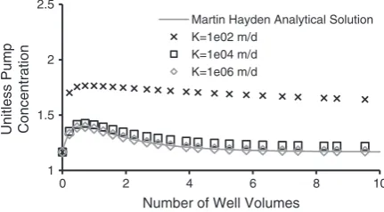
an analytical solution (Martin-Hayden, 2000a). The analytical solution described the temporal variation in pumped sample concentration given a formation concentration that varied linearly from high concentration adjacent to the screen near the pump intake to low concentration at the far end of the screen. A Kwell value of at least 106m/day was required to

provide a close match to both early and late time analytical data (Fig. 2) and account for the delayed arrival of stream lines originating at a distance from the pump intake. AKwellvalue

of 106_{m/day was used for all further scenarios. This value}

is comparable with Kwell estimates using Poiseuille's law

(e.g. (Martin-Hayden, 2000a; Reilly and Gibs, 1993)); assuming fresh water at 12 °C, equivalent conductivities for 5 cm and 10 cm diameter wells are calculated as 5.4 × 107_{m/day and}

2.1 × 108m/day respectively.

Well casing above the open interval was simulated using MODFLOW's wall boundary condition with a very lowKvalue (1 × 10−7m/day) to simulate the impermeable casing with a thickness of 0.01 m. This value was found to be sufficiently low to provide an effectively impermeable barrier with negligible flow observed through the casing relative to the screened interval of the well.

Lower conductivity screens have been shown to have a homogenizing effect on well inflows in a heterogeneous aquifer under pumping conditions (Houben and Hauschild, 2011). Scenarios 6 and 7 were used to investigate the effect of a low-K well screen on well inflows under ambient vertical gradients. Screen conductivity values were chosen arbitrarily to be lower than the surrounding aquifer and were explicitly modeled using MODFLOW's wall boundary condition. Values of 0.5 and 0.05 m/day were chosen for Scenarios 6 and 7 respectively. In all other cases head loss across the screen was assumed negligible and the screen was not modeled.

A single cell within the well screen interval was specified as a well boundary condition to represent the pump intake. The initial pumping rates were either 0.3 or 0.5 l/min (within the range of 0.1_–0.5 l/min recommended for low-flow pumping (Puls and Barcelona, 1996)). Unless otherwise specified, the

1 1.5 2 2.5

0 2 4 6 8 10

Unitless Pump Concentration

Number of Well Volumes

Martin Hayden Analytical Solution K=1e02 m/d

K=1e04 m/d K=1e06 m/d

pump was located in the center of the well screen. During vertical flow simulations, pumping rates were incrementally increased until ambient vertical flows were overcome. The maximum pumping rate used was 36 l/min. Actual modeled pumping rates were half of those stated above due to simulation of half of the model domain.

2.3. Flow simulation

The groundwater flow equations were solved using the PCG2 package of MODFLOW. In order to minimize mass balance errors and artificial oscillations due to very high-K

well cells, head-change and residual-convergence-criteria values were set to 1 × 10−6m and 0.001 m3_/day

respec-tively. Cell-by-cell well in-flows and outflows were obtain-ed directly from the MODFLOW CBB files. Constant-head and volumetric fluxes across the right, front and lower faces of each well grid cell were recorded for each timestep. These flows, in addition to the flows from the right face of the cell immediately to the left of the well cell, allowed the total inflows/outflows in the well to be calculated for each vertical layer. The inflows/outflows were multiplied by two as only half the well was modeled.

Steady-state flows were simulated when comparing well inflows and outflows under unpumped and pumped conditions. Limited transient flow simulations were used to investigate the possible variation in flux distribution as drawdown proceeds and particularly the arrival at the pump intake of water initially in the casing. The 12-h duration of the transient flow simulations was chosen to be significantly longer than the completion of groundwater sampling using well pumping methods (low-flow, or traditional 3–5 well volumes). During the transient simula-tions, the specific yield was set to 0.1 in the aquifer and 1 in the well. Specific storage was specified as 1 × 10−41/m.

2.4. Particle tracking

Particle tracking using the MODPATH 5 (Pollock, 1994) code in time series mode and transient MODFLOW velocity data was used to investigate the temporal variation in the well's capture zone. The relatively low pumping rates and the partially penetrating screens form capture zones that extended only a few meters from the screen. Consequently, particles did not need to be distributed throughout all layers of the model. Particles were placed in up-gradient and down-gradient of the well in layers 10–145 (layers numbered top to bottom). Particles were placed in row 1 on the cell face at the top edge of the model along the plane of symmetry. Particles were released at the onset of pumping and were removed from the model upon arrival at the pump intake. Six particles were placed in each cell (evenly distributed in two rows) in order to provide sufficient resolution for early time (b1 h) capture zones. During particle tracking, porosity within the well was 1 and outside the well 0.25.

2.5. Quantifying the bias to sampling

To allow comparison between vertical flow scenarios it was necessary to quantify the vertical flow induced sample bias. For a particular vertical flow scenario, the bias was calculated by finding the percentage inflow from each layer

and then summing the difference between this and the percentage inflow from each layer under baseline horizontal gradient conditions:

%Bias¼X

n

i¼1

Qvin;i

Qv T

−Q h in;i

Qh T

100 ð1Þ

whereQin,iis the volumetric inflow for the well cell in layeri,QT

is the total volumetric inflow to the well over all layers,nis the number of layers intersected by the well and the superscriptsv

andhindicate vertical flow and ideal horizontal flow conditions respectively.

3. Results and discussion

3.1. Origin of pumped sample water from wells with no ambient vertical_flows

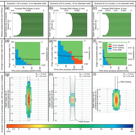
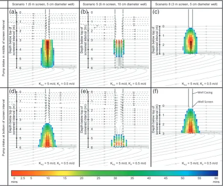
Under horizontal head gradients, flow converges vertically to the well screen since the well is partially penetrating in these scenarios (Fig. 3g–i). This explains the higher influxes at the top and bottom of the well screen during pumping (Fig. 3a–c). However, while the long-time pumping capture zone encapsu-lates the entire well screen (Fig. 3g–i), the time to reach this state depends on the volume of water within the well screen (Fig. 3d–f). For Scenario 1 it takes 2 h to purge all well screen and casing water (Fig. 3d) and achieve a sample comprising 100% formation water. In Scenario 5 it takes over 3 h (Fig. 3e). Even for a well with a 3 m screen, for the low-flow pumping rate used, it takes just over 1 h (Fig. 3f) to purge all non-formation water. In all three cases, to achieve a sample comprising 100% formation water requires purging the equivalent of several screen volumes. However, stabilization of drawdown to within 95% of steady-state drawdown was achieved within 10 min.

After groundwater from the entire screen has reached the pump intake, the pump intake location may not affect the zone of the screen sampled. However, the time to reach this position depends on the well screen volume. In wells with longer screens it can be inferred that prolonged pumping may be required to collect water from the entire screen interval. Until then, pump intake position, pumping rate and pumping duration will play an important role in determining the origin of the water sampled and therefore the sample concentration, even without vertical flows. This result compares well to the modeling of Martin-Hayden et al. (2014) who found that purging of at least two screen volumes was required to obtain a sample consisting of 94% formation water. For the cases considered, well drawdown was not a good indicator of pumping capture zone stabiliza-tion across the screen interval.

3.2. Ambient vertical-flow simulations

3.2.1. Sensitivity of ambient verticalflows in unpumped wells to aquifer and well properties

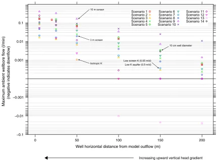
The following observations are made on the vertical flow simulations (and therefore the likelihood of vertical flows occurring in wells) during unpumped conditions (Fig. 4):

1) The farther the well is from the outflow boundary, the smaller the induced vertical flow in the well. In the main body of the aquifer, groundwater flow is predominantly horizontal; upward flows are only seen near the outflow boundary due to convergence of groundwater flow from

deeper in the aquifer. A flow reversal is seen at a distance from the outflow boundary in Scenario 13 where recharge drives downward flow in the well.

2) In the discharge zone, simulated ambient vertical flows are within the observed range reported in the literature for well screens between 3 m and 10 m in length; in fact in the 3 m well the flows are much less than the maximum reported (a simulated value of 0.05 l/min compared with 0.3 l/min observed).

3) Anisotropy/heterogeneities provide a strong control on the degree of vertical flow simulated within the well. Under isotropic conditions, significant vertical flows are not seen until very close to the outflow boundary.

0 0.01 0.02 0 25 50 75 100

0 60 120 180

Dr aw down ( m ) O rig in of pu m p ed w a te r ( % )

Time since pumping started (mins)

-0.015 -0.01 -0.005 0

0

2

4

6

Pumped Well Inflows (L/min)

Dept h below t o p of s c re en ed in te rv al ( m )

-0.02 -0.015 -0.01 -0.005 0

0

1

2

3

Pumped Well Inflows (L/min)

Dept h below t o p of s c re en ed in te rv al ( m ) 0 0.01 0.02 0.03 0.04 0 25 50 75 100

0 60 120 180

Drawdown (m)

Origin of pumped water (%)

Time since pumping started (mins)

-0.01 -0.005 0

0

2

4

6

Pumped Well Inflows (L/min)

Dept h below t o p of s c re en ed in te rv al ( m ) 0 0.01 0.02 0 25 50 75 100

0 60 120 180

Drawdown (m) O ri g in of pu m p ed w a te r ( % )

Time since pumping started (mins)

From Aquifer From Casing From Well 0 1 2 3 4 5 6 Dept h below t o p of s c re en ed in te rv al (m ) 0 1 2 3 4 5 6 Dept h below t o p of s c re en ed in te rv al (m ) 0 1 2 3 Dept h below t o p of s c re en ed in te rv al (m ) 55 50 45 40 35 30 25 20 15 10 5 2.5 0 mins 60 mins Kx,y= 5 m/d,

Kz= 0.5 m/d

Kx,y= 5 m/d,

Kz= 0.5 m/d

Kx,y= 5 m/d,

Kz= 0.5 m/d

(a)

(b)

(c)

(d)

(e)

(f)

(g)

(h)

(i)

Scenario 1 (6 m screen, 5 cm diameter well) Scenario 5 (6 m screen, 10 cm diameter well) Scenario 8 (3 m screen, 5 cm diameter well)

Steady-statepumped well inflows

Change in sample origin with time

Well Screen

Well Casing

Evolution of source of pumped water with time (pump in middlel)

-0.015 -0.01 -0.005 0

0

2

4

6

Pumped Well Inflows (L/min)

Dept h below t o p of s c re en ed in te rv al ( m )

4) Increasing well volume (length or diameter) increases the magnitude of vertical flows, with screen length having a greater effect as the head difference between opposite ends of the screen is greater.

5) Lower aquiferKvalues reduce flows into and out of the well and hence decrease vertical flows in the well. Reducing screen K has a similar effect. However, care should be taken if undertaking pumped sampling in low permeability settings or with a lowKscreen in order to prevent excessive drawdown.

Typical ambient vertical flow patterns in the well were similar to those noted by others (Konikow and Hornberger, 2006; Reilly et al., 1989; Segar, 1993), with inflows biased towards the region of highest head intersected by the well screen (the bottom of the well in this case) and outflows towards that of lowest head (the top of the well screen) (Fig. 5a). A gradual reduction of inflows and increase of outflows is observed between these two points. If the hydraulic conductivity distribution is not homogenous, inflows and outflows may still be biased towards zones of higher conductivity intersected by the well screen (Fig. 5b).

3.2.2. Origin of pumped sample water from wells with ambient verticalflows

With increasing vertical flows, pumping may not be able to counteract the vertical head gradients that generate ambient upflow in the well. The sample origin becomes biased towards

the ambient inflowing zones in the well (e.g., results from Scenario 1, 5 and 8,Fig. 6).

For Scenario 8 (3 m screen) pumping at 0.3 l/min is sufficient to partially overcome the ambient vertical head gradients generating a maximum ambient upflow in the well of 0.05 l/min (Fig. 6c, f). Like the baseline case (Fig. 3i), at long times the sample is drawn from the entire screen interval and is independent of the pump intake position. However, it requires over 60 min of pumping to reach this position. Unlike the baseline case, the sample origin does not depend only on the formation hydraulic conductivity distribution. The sample remains partially biased towards the zone of highest head intersected by the screen with a greater portion of the sample being drawn from the bottom of the screen interval.

In Scenario 1, with maximum ambient upflow in the well of 0.16 l/min, pumping at 0.3 l/min is insufficient to overcome the ambient vertical head gradients (Fig. 6a, d). Even after extended pumping, the pumped sample is drawn entirely from the bottom half of the screen interval. Like Scenario 8 (Fig. 6c, f), at long times the origin of the sample in the screen interval is independent of the pump intake position. During pumped sampling, ambient upflow, driven by the ambient vertical head gradient, continues in the upper portion of the screened interval of the well. This water bypasses the pump intake entirely; even if mixing with casing water were to occur, there will be no bias to the sample in this case.

Unlike the two previous cases, for Scenario 5, with ambient upflow in the well of 0.19 l/min, pump intake Well horizontal distance from model outflow (m)

Maximum ambient wellbore flow (l/min)

(negative indicates downflow)

−0.1 −0.01 −0.001 0.001 0.01 0.1

0 50 100 150 200

Increasing upward vertical head gradient

position is important even after extended pumping. Different portions of the aquifer are sampled when the pump intake is positioned in the middle (Fig. 6b) or the bottom of the screen interval (Fig. 6e). With the pump intake located at the

bottom of the screen interval (the zone of the screen with highest inflow), the pumped sample is drawn from only the bottom third of the well. Any ambient flows entering farther up the well screen bypassing the pump intake entirely 0

1

2

3

4

5

6

-0.03 -0.015 0 0.015 0.03

Depth below top of _{screened interval (m)} Well Inflows & Outflows (L/min)

Inflows Outflows

0

1

2

3

4

5

6

-0.03 -0.015 0 0.015 0.03

Depth below top of _{screened interval (m)} Well Inflows & Outflows (L/min)

Inflows Outflows

(b)

(a)

Fig. 5.Simulated ambient well inflows/outflows under vertical head gradients for: (a) Scenario 1 (6 m well screen, 1:10 anisotropy) and, (b) Scenario 11 (6 m well, 1.5 m thick lowKlayer intersecting the middle of the well) with the well located 5 m from the outflow boundary.

(a)

(b)

(c)

(d)

(e)

(f)

(Fig. 6e). Moving the pump intake to the middle of the well screen (Fig. 6b), the zone of the well with highest flow, allows a mixture of the entire inflowing zone of the screen to be sampled. This maximizes the portion of the aquifer sampled but gives a more mixed sample.

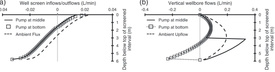
The pump intake position has very little effect on the well inflows and outflows during pumping (Fig. 7a). The differ-ence in sample composition due to the pump intake location is clearer when considering the patterns of vertical flows in the well during pumping (Fig. 7b). When the pump intake is located in the middle of the screened interval, 0.045 l/min of groundwater entering the well through the lower half of the screen interval flows past the pump intake during pumping. The volume of water not captured by the pump depends on the rate of ambient vertical flows in the well.

As suggested by (Greswell et al. (in press)), in wells with high ambient vertical flows, pumped sampling at low rates can be thought of as almost analogous with taking a passive sample when compared with the volumes of groundwater flowing passed the pump intake. Groundwater not captured by pumping will exit the well higher up in the screen interval. The pumped sample composition will depend on the degree of in-well mixing between streamlines originating from different screen intake points. If lateral dispersion and mixing between streamlines in the well are low, sampling may only draw from a subset of upward flowing streamlines. If the pumped sample does not represent a fully mixed snapshot then horizontal position of the pump intake in the well becomes important in sample origin and sample repeatability. It can be inferred that dispersion and mixing are also important if the pump intake is located at the top of the well. The sample origin will depend on what water is carried to the pump intake, what water exits the well screen lower down, and the degree of mixing between waters of different origin moving upwards in the screen interval. If full mixing between streamlines can be assured, taking multiple samples at different depths in the screened portion of the well may be a way of assessing vertical changes in water quality from different screen inflow points.

3.2.3. The transition from baseline conditions to vertical ambient head gradient biased samples

As ambient upflow increases, a transition from permeability-weighted sampling conditions to vertical head gradient biased

conditions occurs. The sample becomes increasingly biased towards the zone of the screen intersecting the region of highest head (Fig. 8a). For a fixed pumping rate, sample origin depends on the rate of ambient upflow in the well. However, sample bias does not occur only when ambient vertical flows in the well are much greater than the pumping rate. For example, considering Scenario 1 (Fig. 8a), the sample origin begins to become biased towards the zone of highest head intersecting the screen for ambient vertical flows in the well of only 0.01 l/min. Once the maximum ambient flow in the well reaches 0.07 l/min the inflow to the well is zero at the top of the screen during pumping. As the maximum ambient upflow increases to 0.15 l/min (50% of the pumping rate) the sample origin is dominated by the ambient vertical hydraulic gradient and the sample is drawn from the bottom half of the screen interval only.

Comparing the percentage bias to the pumped sample due to ambient vertical flows (Eq.(1)) against the maximum ambient upflow in the well, a similar pattern is observed for all scenarios (Fig. 8b). As the maximum ambient upflow in the well increases from 0% to 50% of the pumping rate the percentage bias increases. A transition between baseline sampling conditions and vertical head gradient biased conditions occurs. Within this transition zone sample origin is very sensitive to ambient upflow rates. If ambient vertical flows in the well vary (e.g. seasonally), sample origin during pumped sampling will differ even if fixed sampling proce-dures are used. A similar conclusion is drawn byRiley et al. (2011)for tracer testing in the presence of vertical flows.

As the maximum ambient upflow in the well increases beyond 50% of the pumping rate, the percentage bias to sampling levels off. The well inflows are determined by the ambient vertical head gradients with pumping having little ability to counteract vertical flows in the well. Changes in ambient vertical flow rates become less important to the sample origin, pump position becomes important even at long times and pumped sampling becomes increasingly analogous to a passive sample.

3.2.4. Overcoming ambient vertical_flow bias via increased pumping

If a well sampling is undertaken at higher pumping rates, vertical gradients can be overcome and the sample can be drawn from the entire screen interval. For Scenario 1, with

0

1

2

3

4

5

6

-0.04 -0.02 0 0.02 0.04

Depth below top of screened

interval (m)

Well screen inflows/outflows (L/min)

Pump at middle

Pump at bottom

Ambient Flux

0

1

2

3

4

5

6

-0.4 -0.2 0 0.2 0.4

Depth below top of screened

interval (m)

Vertical wellbore flows (L/min)

Pump at middle

Pump at bottom

Ambient Upflow

(b)

(a)

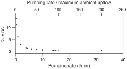
maximum ambient upflow in the well of 0.16 l/min, pumping at 0.3 l/min results in vertical flow bias of 14% (Fig. 9). Increasing the pumping rate to 2 l/min reduces the ambient vertical flow induced bias tob10%. However, achieving a 10% bias does not provide a sample drawn from the entire screen interval (Fig. 8a). The pumping rate has to be increased to 10 s·l/min to approach 0% bias and achieve a permeability-weighted sample unbiased by ambient vertical head gradients. The pumping rate required to fully overcome vertical head gradients is many tens of times the vertical head gradient driven ambient upflow in the well.

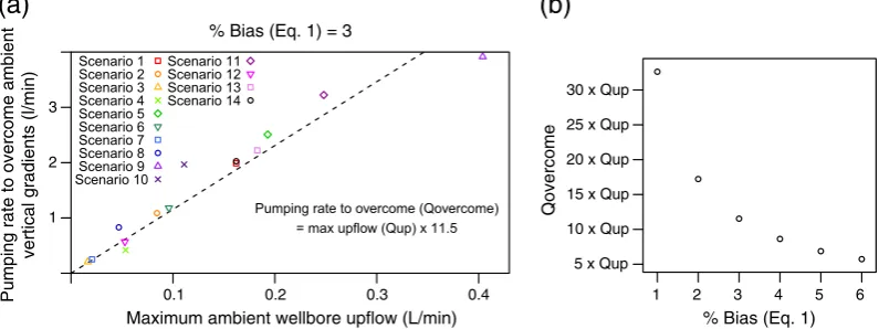
Using the simulated maximum ambient upflow in the well to compare all scenarios, a linear relationship exists between the maximum ambient upflow simulated in the well and the pumping rate required to overcome the vertical gradient induced bias. For example, to reduce the ambient vertical flow induced sampling bias to 3% (Eq. (1)) it is necessary to pump at 11.5 times the maximum ambient upflow rate in the well (Fig. 10a). Similar linear relationships exist for other percentage biases (Fig. 10b). As observed for Scenario 1 (Fig. 9), it is necessary to use a pumping rate of tens of times the ambient vertical flow rate in the well to fully overcome ambient vertical head gradients and achieve a bias

approaching zero. Hence, for the modeling scenarios consid-ered, knowledge of the maximum ambient upflow in the well is enough to estimate the pumping rate required to overcome the in-well vertical flows. Detailed knowledge of the flow distribution was not required.

The implication for groundwater sampling in wells with maximum ambient upflow in the range observed by (Elci et al., 2001) (0.015–2.3 l/min) is that low-flow sampling will be biased towards the zones of highest head intersecting the screen. Increasing the pumping rates to several liters per minute may not fully overcome the ambient vertical head gradients observed. To obtain a permeability-weighted sample from across the screen interval during pumped sampling in these wells the pumping rate may need to be tens of liters per minute or higher.

4. Conclusions

Numerical modeling to evaluate the effect of ambient vertical flows on groundwater sampling using pumps has demonstrated that naturally occurring vertical flows of the magnitude reported in literature may be a key control on sample origin even in wells with screensb10 m in length. If permeability-weighted sampling from across the screen interval is the goal it may be necessary to pump at rates many times the ambient vertical flow rate in the well. Purging at low pumping rates such as those recommended for low-flow sampling would not be sufficient. Ambient vertical flows in the wellbore are increased by:

1) greater aquifer hydraulic conductivity and greater aquifer depth;

2) greater proximity to discharge (or recharge) zones; 3) greater well volume (well diameter and length), screen

hydraulic conductivity;

4) and greater vertical/horizontal hydraulic conductivity anisotropy (including the presence of discrete layers of low permeability).

Inflow per layer (L/min)

Depth below top of screened interval (m)

0

1

2

3

4

5

6

−0.020 −0.015 −0.010 −0.005 0.000

Max Upflow (L/min)

0.00 0.01 0.07 0.15 0.16

% Bias (Eq. 1) 0 2 8 13 14

(a)

Maximum ambient wellbore upflow / pumping rate (%)

% Bias (Eq. 1) from baseline case

1 2 3 4 5 6 8 10 20 30 40 50

0 50 100 150

Scenario 1 Scenario 2 Scenario 3 Scenario 4 Scenario 5 Scenario 6 Scenario 7

Scenario 8 Scenario 9 Scenario 10 Scenario 11 Scenario 12 Scenario 13 Scenario 14

(b)

Fig. 8.Departure from no vertical flow baseline as a function of ambient upflow in the well: (a) deviation from baseline (Eq.(1)) and variation in pumped influxes for Scenario 1 (Q = 0.3 l/min), (b) deviation from baseline conditions for all scenarios.

Pumping rate (l/min)

% Bias

0 5 10

0 10 20 30 40

0 50 100 150 200 250

Pumping rate / maximum ambient upflow

For situations where the maximum ambient upflow in the well is b5% of the pumping rate the numerical modeling undertaken here has demonstrated that:

1) it is possible to overcome ambient vertical gradients, even with low-flow pumping, and achieve a sample drawn from the entire screen interval;

2) pumping rate and time (which can be significant in sampling terms) are important controls on sample origin (this is the case even without vertical flows);

3) and during early pumping the sample origin will depend on pump intake position but at long times may be pump independent.

As ambient upflow in the well increases towards 50% of the pumping rate, a transition occurs. The sample becomes increasingly biased towards the zone of highest head intersecting the screen. In these cases:

1) water may not be drawn from the entire saturated screen interval even with extended pumping times;

2) if ambient vertical flow rates vary (e.g. seasonally), the sample origin may vary even if pump intake position, pump rate and pump time are fixed;

3) pump intake position is important in determining the sample origin, this may be the case even after an extended pumping period;

4) targeting the zone of the well with maximum vertical flow maximizes the vertical extent of aquifer sampled.

For wells with ambient upflow rates much greater than the pumping rate the sample is entirely biased towards the zone of highest head. The pumped sample becomes analo-gous to a passive sample. In these cases:

1) pumping rate and time are not important;

2) pump intake position is the key control on the sample origin

3) sampling from the base of a borehole provides a more discrete sample from that inflow zone, and through appropriate choice of sampling location might enable level-determined sampling

4) however, quantitative predictions of water quality varia-tion with depth will depend on assessing the degree of

dispersion and mixing as water of different origins enters and exits the well screen

Vertical flows can introduce considerable uncertainty when attempting to relate sample concentration to in-aquifer conditions, even in wells with screens b10 m in length. Knowledge of the ambient vertical flow rate in the well can be used, in conjunction with sampling objectives, to guide decisions on pumping rate, pumping duration and pump intake location. From a practitioner community viewpoint, sampling objectives will determine if a detailed knowledge of sample origin is required. If this detailed knowledge is required then supporting vertical flow investi-gations are recommended.

Acknowledgments

This work forms part of an Open Case Studentship supported by the Natural Environment Research Council

[grant number NE/H019170/1] and Case partners

Waterra-In-Situ (now In-Situ Europe Ltd) and the Environ-ment Agency (for England). We acknowledge the generosity of ESI Ltd for providing access to their Groundwater Vistas software. Finally, we thank two reviewers for their comments which greatly improved this manuscript.

References

ASTM International, 2013. Standard guide for sampling ground-water monitoring wells, D4448-01.

Barber, C., Davis, G.B., 1987. Representative sampling of ground water from short-screened boreholes. Ground Water 25 (5), 581–587.http://dx.doi. org/10.1111/j.1745-6584.1987.tb02888.x.

Barcelona, M.J., Wermann, H.A., Varljen, M.D., 1994. Reproducible well-purging procedures and VOC stabilization criteria for ground-water sampling. Ground Water 32 (1), 12–22. http://dx.doi.org/10.1111/j. 1745-6584.1994.tb00605.x.

Barcelona, M.J., Varljen, M.D., Puls, R.W., Kaminski, D., 2005. Ground water purging and sampling methods: history vs. hysteria. Ground Water Monit. Rem. 25 (1), 52–62.http://dx.doi.org/10.1111/j.1745-6592.2005. 0001.x.

Brassington, F.C., 1992. Measurements of head variations within observation boreholes and their implications for groundwater monitoring. Water Environ. J. 6 (3), 91–100.http://dx.doi.org/10.1111/j.1747-6593.1992. tb00742.x.

BS ISO, 2009.Water quality–Sampling–Part 11: Guidance on Sampling of

Groundwaters, BS ISO 5667–11:2009, (40 pp.).

% Bias (Eq. 1) = 3

Maximum ambient wellbore upflow (L/min)

Pumping rate to overcome ambient

vertical gradients (l/min)

1 2 3

0.1 0.2 0.3 0.4

(a)

% Bias (Eq. 1)

Qovercome

5 x Qup 10 x Qup 15 x Qup 20 x Qup 25 x Qup 30 x Qup

1 2 3 4 5 6

(b)

BS ISO, 2010.Water quality–Sampling–Part 22: Guidance on the Design and

Installation of Groundwater Monitoring Points, BS ISO 5667–22, (36 pp.).

Church, P.E., Granato, G.E., 1996. Bias in ground-water data caused by well-bore flow in long-screen wells. Ground Water 3 (2), 262–273.http://dx. doi.org/10.1111/j.1745-6584.1996.tb01886.x.

Dumble, P., Fuller, M., Beck, P., Sojka, P., 2006. Assessing contaminant migration pathways and vertical gradients in a low-permeability aquifer

using multilevel borehole systems. Land Contam. Reclam. 14 (3), 699–712.

Elci, A., Molz, F.J.I., Waldrop, W.R., 2001. Implications of observed and simulated ambient flow in monitoring wells. Ground Water 39 (6), 853–862.http://dx.doi.org/10.1111/j.1745-6584.2001.tb02473.x. Elci, A., Flach, G.P., Molz, F.J., 2003. Detrimental effects of natural vertical

head gradients on chemical and water level measurements in observa-tion wells: identificaobserva-tion and control. J. Hydrol. 28, 70–81.http://dx.doi. org/10.1016/S0022-1694(03)00201-4.

Furlong, B.V., Riley, M.S., Herbert, A.W., Ingram, J.A., Mackay, R., Tellam, J.H., 2011. Using regional groundwater flow models for prediction of regional wellwater quality distributions. J. Hydrol. 398 (1–2), 1–16.http://dx.doi. org/10.1016/j.jhydrol.2010.11.022.

Giddings, T., 1987. What is an adequate screen length for monitoring wells? Ground Water Monit. Rem. 7 (2), 96–103.http://dx.doi.org/10.1111/j. 1745-6592.1987.tb01049.x.

Greswell, R.B., Durand, V., Aller, M.F., Riley, M.S., Tellam, J.H., 2014. A method of conducting simultaneous convergent tracer tests in a multilayered sand-stone aquifer. Ground Water (http://dx.doi.org/doi:101111/gwat, in press). Harbaugh, A.W., Banta, E.R., Hill, M.C., McDonald, M.G., 2000. Modflow

−2000. The U.S. Geological Survey Modular Ground−Water Model−

User Guid to Modularization Concepts and the Ground−Water Flow Process, USGS Open−File Report, pp. 00–92 http://pubs.usgs.gov/of/ 2000/0092/report.pdf.

Houben, G.J., Hauschild, S., 2011. Numerical modeling of the near−field hydraulics of water wells. Ground Water 49 (4), 570–575.http://dx.doi. org/10.1111/j.1745-6584.2010.00760.x.

Hutchins, S.R., Acree, S.D., 2000. Ground water sampling bias observed in shallow, conventional wells. Ground Water Monit. Rem. 18, 86–93. http://dx.doi.org/10.1111/j.1745-6592.2000.tb00255.x.

Kaleris, V., Hadjitheodorou, C., Demetracopoulos, A.C., 1995. Numerical simulation of field methods for estimating hydraulic conductivity and concentration profiles. J. Hydrol. 171 (3–4), 319–353.http://dx.doi.org/ 10.1016/0022-1694(94)06012-T.

Konikow, L.F., Hornberger, G.Z., 2006. Modeling effects of multinode wells on solute transport. Ground Water 44 (5), 648–660.http://dx.doi.org/10. 1111/j.1745-6584.2006.00231.x.

Kozuskanich, J., Novakowski, K.S., Anderson, B.C., 2012. Influence of piezometer construction of groundwater sampling in fractured rock. Ground Water 50 (2), 266–278.http://dx.doi.org/10.1111/j.1745-6584. 2011.00840.x.

Lacombe, S., Sudicky, E.A., Frape, S.K., Unger, A.J.A., 1995. Influence of leaky boreholes on cross-formational groundwater flow and contaminant transport. Water Resour. Res. 31 (8), 1871–1882.http://dx.doi.org/10. 1029/95WR00661.

Ma, R., Zheng, C., Tonkin, M., Zachara, J.M., 2011. Importance of considering intraborehole flow in solute transport modeling under highly dynamic flow conditions. J. Contam. Hydrol. 123 (1–2), 11–19.http://dx.doi.org/ 10.1016/j.jconhyd.2010.12.001.

Martin-Hayden, J.M., 2000a. Sample concentration response to laminar wellbore flow: implications to ground water data variability. Ground Water 89 (1), 12–19.http://dx.doi.org/10.1111/j.1745-6584.2000.tb00197.x.

Martin-Hayden, J.M., 2000b. Controlled laboratory investigations of wellbore concentration response to pumping. Ground Water 38 (1), 121–128. http://dx.doi.org/10.1111/j.1745-6584.2000.tb00209.x.

Martin-Hayden, J.M., Wolfe, N., 2000. A novel view of wellbore flow and partial mixing: digital image analyses. Ground Water Monit. Rem. 20 (4), 96–103.http://dx.doi.org/10.1111/j.1745-6592.2000.tb00294.x. Martin-Hayden, J.M., Plummer, M., Britt, S.L., 2014. Controls of wellbore flow

regimes on pump effluent composition. Ground Water Monit. Rem. 52 (1), 96–104.http://dx.doi.org/10.1111/gwat.12036.

Mayo, A.L., 2010. Ambient well-bore mixing, aquifer cross-contamination, pumping stress, and water quality from long-screened wells; what is sampled and what is not? Hydrogeol. J. 18 (4), 823–837.http://dx.doi. org/10.1007/s10040-009-0568-2.

Metcalf, M.J., Robbins, G.A., 2007. Comparison of water quality profiles from shallow monitoring wells and adjacent multilevel samplers. Ground Water Monit. Rem. 27 (1), 84–91. http://dx.doi.org/10.1111/j.1745-6592.2006.00126.x.

Pollock, D.W., 1994. User's Guide for MODPATH/MODPATH-PLOT, Version 3: A particle tracking post-processing package for MODFLOW, the U.S. Geological Survey finite-difference ground-water flow model, Open-File Report. U.S. Geological Survey, Reston, Virginia, pp. 94–464http://water. usgs.gov/nrp/gwsoftware/modpath5/ofr94464.pdf.

Puls, R.W., Barcelona, M.J., 1996.Low-Flow (Minimal Drawdown) Ground-Water Sampling Procedures. EPA/540/S-95/504.

Reilly, T.E., Gibs, J., 1993. Effects of physical and chemical heterogeneity on water-quality samples obtained from wells. Ground Water 31 (5), 805–813.http://dx.doi.org/10.1111/j.1745-6584.1993.tb00854.x. Reilly, T.E., Franke, O.L., Bennett, G.D., 1989. Bias in groundwater samples caused

by wellbore flow. Journal of Hydraulic Engineering 115 (2), 270–276.http:// dx.doi.org/10.1061/(ASCE)0733-9429(1989)115:2(270).

Riley, M.S., Tellam, J.H., Greswell, R.B., Durand, V., Aller, M.F., 2011. Convergent tracer tests in multilayered aquifers: the importance of vertical flow in the injection borehole. Water Resour. Res. 47.http://dx.

doi.org/10.1029/2010WR009838(14 pp.).

Rivett, M.O., Lerner, D.N., Lloyd, J.W., 1990. Temporal variations of chlorinated solvents in abstraction wells. Ground Water Monit. Rem. 10 (4), 127–133.http://dx.doi.org/10.1111/j.1745-6592.1990.tb00029.x. Robbins, G.A., Martin-Hayden, J.M., 1991. Mass balance evaluation of monitoring well purging: Part I. Theoretical models and implications for representative sampling. J. Contam. Hydrol. 8, 203–224.http://dx. doi.org/10.1016/0169-7722(91)90020-2.

Segar, D.A., 1993.The effect of open boreholes on groundwater flows and chemistry. Unpublished PhD Thesis, University of Birmingham, p. 289. Stone, W.J., 1997. Low-flow ground water sampling—is it a cure-all? Ground

Water Monit. Rem. 17 (2), 70–72. http://dx.doi.org/10.1111/j.1745-6592.1997.tb01278.x.

Streetly, H.R., Hamilton, A.C.L., Betts, C., Tellam, J.H., Herbert, A.W., 2002. Reconnaissance tracer tests in the Triassic sandstone. Q. J. Eng. Geol. Hydrogeol. 35, 167–178.http://dx.doi.org/10.1144/1470-9236/2000-30. Taylor, R.G., Cronin, A.A., Trowsdale, S.A., Baines, O.P., Barrett, M.H., Lerner, D.N., 2006. Vertical groundwater flow in Permo-Triassic sediments underlying two cities in the Trent River Basin (UK). J. Hydrol. 284, 92–113.http://dx. doi.org/10.1016/S0022-1694(03)00276-2.

US EPA, 2010. Low Stress (Low Flow) Purging and Sampling Procedure for the Collection of Groundwater Samples from Monitoring Wells, EPASOP-GW 001.http://www.epa.gov/region1/lab/qa/pdfs/EQASOP-GW001.pdf. Varlijen, M.D., Barcelona, M.J., Obereiner, J., Kaminski, D., 2006. Numerical simulations to assess the monitoring zone achieved during low-flow purging and sampling. Ground Water Monit. Rem. 26 (1), 44–52.http:// dx.doi.org/10.1111/j.1745-6592.2006.00029.x.