Behaviour of a Shear-Wave at a Solid-Smectic Interface
B. C. Snow and I. W. Stewart
Department of Mathematics and Statistics, University of Strathclyde,
Glasgow, Scotland, United Kingdom
Abstract
Results of theoretical investigations into the behaviour of a shear wave at the boundary between an isotropic solid and a smectic A liquid crystal are presented. These results track the subsequent response of the smectic to the refracted wave. Using the techniques of Landau and Lifshitz for sound in isotropic fluids [1], we extend the results for smectic C by Gill and Leslie [2] and perform the analogous calculations for a sample of smectic A using the dynamic theory of Stewart [3]. These calculations enable a comparison between the results for smectic A and an extension, by the present authors, to the known results for smectic C.
Motivated by the work of Auernhammer, Brand, and Pleiner [4, 5], mechanisms for determining the impact of perturbations upon the modes of response behaviour will be analysed, with plots demonstrating the amplitudes of these waves relative to that of the incident wave displayed for a range of typical physical parameters characteristic to smectic C and smectic A.
1
Introduction
It is well known that smectic liquid crystals have the potential for much faster switching than their nematic counterparts. As was remarked by Gill and Leslie [2], induced flow can play a major role in the dynamics of such switching, and it is therefore of great interest to develop a comprehensive understanding of how smectics behave when subjected to a variety of perturbations and induced flow profiles.
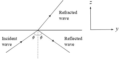
The analysis presented herein will consider a perturbation to a sample of bookshelf aligned smectic A (SmA) induced by a shear wave incident at the plane interface between the smectic and an isotropic elastic solid such that the wave first propagates through the solid then undergoes a reflection and refraction on contact with the interface, as shown in Fig. 1.
z
y
ϕ ϕ
Incident wave
[image:1.612.185.434.579.700.2]Reflected wave Refracted wave
Section 2 will provide a brief outline of Stewart’s dynamic theory for SmA [3]. Section 3 will provide, in an analogous manner to that adopted by Gill and Leslie [2] for smectic C (SmC), derivations of the dispersion relations for the reflected and refracted waves, together with the consequent interfacial conditions to be utilised in the analysis. A brief summary of the results from [2] will be presented in Section 4, before deriving, in Section 5, expressions that relate the amplitudes of the reflected and refracted waves in terms of the incident wave amplitude and material parameters that characterise SmA and SmC, the latter being a novel extension to the work in [2]. Section 5 concludes with plots which demonstrate how the amplitudes of the refracted waves vary with the incident angular frequency of the incident wave. The paper will close with a summary and discussion of the main results and the potential influence on further work.
2
Continuum Theory for Smectic A Liquid Crystals
It is known that nematic liquid crystals consist of rod-like molecules that tend to align parallel to each other along some common preferred direction indicated by the unit vector n, called the director. The SmA liquid crystal phase occurs when the constituent molecules are arranged in layers, where the director is, on average, generally aligned perpendicular to the local layer structure and is parallel to the local layer normal. In SmC liquid crystals the director is tilted at an angle θ relative to the layer normal; θ is usually temperature dependent and is called the smectic cone angle. The director ncontinues to be defined as the average direction of the molecular alignment and, from the physical point of view,nand −nare indistinguishable. It is the SmA phase that is the main concern here, although a comparison with results for SmC will also be made.
We now summarise the continuum theory in [3], in which n and a are allowed to separate, as considered by Ribotta and Durand [6]. The standard suffix notation for Cartesian vectors and tensors [7] is employed. SmA is described by two unit vectors: the layer normalaand the director
n. The layer normal is perpendicular to the plane of the smectic layers, and it is conveniently defined via a scalar function Φ(x, y, z, t) such that
a= ∇Φ
|∇Φ|, i.e., ai =
Φ,i
|∇Φ|, (2.1)
from which is it clear thata is a unit vector by its definition. As mentioned,nis also constrained to be a unit vector, so that
n·n=nini = 1. (2.2)
We will be concerned with samples which are both isothermal and incompressible (in the classical sense); the latter of these requires that the velocity v at any point in the smectic satisfies
vi,i = 0. (2.3)
The balance of linear momentum takes the form
ρvi˙ =ρfi−p,i˜ + ˜gjnj,i+Gjnj,i+|∇Φ|aiJj,j+ ˜tij,j, (2.4)
withρ denoting the density, fi the external body force per unit mass, ˜p=p+wA, where p is the pressure andwA is the elastic energy density given by [8]
wA= 12K1a(∇ ·a)2+12K1n(∇ ·n−s0)2+12K2∇ ·[(n· ∇)n−(∇ ·n)n]
+12B0|∇Φ|−2(1− |∇Φ|)2+12B1
1−(n·a)2
+B2(∇ ·n) 1− |∇Φ|−1
, (2.5)
the director saddle–splay; B0 is the layer compression constant, B1 is the constant attributed to coupling betweennanda, and B2 characterises the energy due to the coupling between splay and layer compression. The superposed dot represents the usual material time derivative. The term ˜tij is the viscous stress with components
˜
tij =α1(nkAklnl)ninj+α2Ninj+α3niNj+α4Aij +α5(njAiknk+niAjknk)
+ (α2+α3)niAjknk+τ1(akAklal)aiaj+τ2(aiAjkak+ajAikak) +κ1(aiNj+Niaj+niAjkak−njAikak) +κ2(nkAklnl)(niaj+ainj)
+κ3[(nkAklnl)aiaj+ (akAklal)ninj]
+κ4[2(nkAklal)ninj+ (nkAklnl)(ainj+niaj)]
+κ5[2(nkAklal)aiaj+ (akAklal)(niaj +ainj)]
+κ6(njAikak+niAjkak+aiAjknk+ajAiknk). (2.6)
The coefficients on the right-hand side of (2.6) are dynamic viscosities, whileAij denotes the usual rate of strain tensor, with components
Aij = 12(vi,j+vj,i),
andN is the co-rotational time flux, defined asNi = ˙ni−Wijnj, whereWij is the vorticity tensor whose components are given by
Wij = 12(vi,j−vj,i).
The term ˜gi is a dynamic contribution given by
˜
gi=−(α3−α2)Ni−(α2+α3)Aijnj−2κ1Aijaj, (2.7)
andGi is the generalised external body force, which is related to the external body momentKi per unit mass via
ρKi=ijknjGk. (2.8)
The vectorJ is the negative of the permeative force τ, and has components as
Ji =−∂wA ∂Φ,i
+ 1
|∇Φ|
"
∂wA ∂aj,k
,k
−∂wA ∂aj
#
(δji−ajai), (2.9)
The balance of angular momentum may be expressed in the form
∂wA ∂ni,j
,j
−∂wA ∂ni
+ ˜gi+Gi =λni, (2.10)
whereλis a Lagrange multiplier arising from the unit vector constraint on nas given in equation (2.2), which can generally be either evaluated or eliminated on taking the scalar product of (2.10) withn. The permeation equation, which describes permeative flow between the smectic layers, is
˙
Φ =−λpJi,i, (2.11)
whereλp≥0 is the permeation coefficient.
3
Reflection and Refraction of the Shear Wave at the
Solid-Smectic A Interface
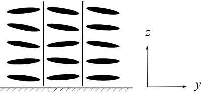
z
[image:4.612.204.411.41.136.2]y
Figure 2: Problem set-up for “bookshelf” SmA.
assume the solid and smectic to be unbounded in space. Referred to the geometry of Fig. 1, the initially undistorted sample of bookshelf aligned SmA will have its configuration described by
n=n0= (0,1,0), Φ = Φ0 =y. (3.1)
This initial configuration will be perturbed by an incident shear wave with displacement u = (ux, uy, uz) whose components are
ux=Aexp{i[ωt−k(ysinφ+zcosφ)]}, uy =uz = 0, (3.2)
whereAis the constant (real, without loss of generality) amplitude of the wave andφis the constant angle of incidence (to the interface’s normal);ω and k denote the constant incident frequency and wave number, respectively. This displacement is required to satisfy the wave equation for an isotropic solid [9, p. 87]. For the displacement as given in (3.2), this leads to the relation
ρsω2 =µsk2, (3.3)
whereµsandρsdenote, respectively, the shear modulus (or bulk modulus) and density of the solid. It is natural to suppose that the displacement of the reflected waveur = (ur
x, ury, urz) takes the form
urx=Bexp{i[ωt−k(ysinφ−zcosφ)]}, ury =urz = 0, (3.4)
withB a constant complex amplitude which will be determined below.
It is expected that the incident wave will induce a perturbation to the smectic. It will be assumed that this disturbance may cause small changes to the alignment of the constituent molecules (that is, to the director) and to the layer normal. The refracted wave velocity in the smectic is assumed to be of the form
vx =vexp{i[ωt−k(ysinφ+qz)]}, vy =vz = 0, (3.5)
with v, q ∈ C to be determined below. Note that this form of v automatically satisfies the incompressibility conditionvi,i = 0. The perturbed scalar Φ will be given by
Φ =y−u(y, z, t), (3.6)
for small perturbationsu= ˆuexp{i[ωt−k(ysinφ+qz)]}such that|uˆ| 1. Then, to first order in uand derivatives thereof,
a= ∇Φ
|∇Φ| = (0,1,−uz). (3.7)
Finally, the directorn= (nx, ny, nz) is perturbed so that
nx =nexp{i[ωt−k(ysinφ+qz)]}, ny = 1, nz = 0. (3.8)
Substitution of (3.5) to (3.8) into the balance laws for linear and angular momentum (2.4) and (2.10) as well as the permeation equation (2.11) leads to the requirement ˆu ≡0. Therefore a≡ (0,1,0) to first order. Further, two dispersion relations are identified:
2iρω+k2 α4q2−ηsin2φ
v−2ωk(α2+κ1)nsinφ= 0, (3.9)
where
η=α2−α4−α5−τ2+ 2(κ1−κ6), (3.11)
upon identification of λas B1 and with the pressure reducing to an arbitrary function of time t. Equations (3.9) and (3.10) furnish us with non-trivial solutions forv and nprovided the relation
2iρω+k2(α4q2−ηsin2φ)
[(α2−α3)ω−B1] + 2ωk2(α2+κ1)2sin2φ= 0 (3.12)
is satisfied. Rearranging this forq2 yields
q2 =β1−2iβ2, (3.13)
whereβ1 and −2β2 are the real and imaginary parts of q2, respectively, given by
β1 =
η+2ω(α2+κ1) 2
B1+γ1ω
sin2φ, β2= ρξ α4
, (3.14)
and we have introduced the notation
ξ =ω/k2, (3.15)
for later comparison with [2]. Equation (3.13) yields two solutions for q. To ensure bounded solutions, it is clear from the forms of the perturbed quantities that the root with negative imaginary part is required here. One therefore finds
q=χ−iψ, ψ >0, (3.16)
where
χ= β2
ψ, ψ=
s
1 2
q
β2
1+ 4β22−β1
. (3.17)
Note that normal incidence gives
q|φ=0 = (1−i)
r
ρξ α4
. (3.18)
Boundary Conditions
Continuity of velocity and surface traction are imposed at the interface. Using the above expressions for displacement in the solid of the incident and reflected waves in (3.2) and (3.4), respectively, combined with equation (3.5), continuity of velocity leads to the relation
iω(A+B) =v. (3.19)
In the solid, the surface traction is required to satisfy the constitutive equations for isotropic elasticity [10, p. 115], so that continuity of surface traction at the interface imposes the requirement
2µs(A−B) cosφ=α4qv. (3.20)
[image:5.612.86.537.320.443.2]4
The Smectic C Case
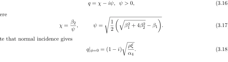
Figure 3 depicts a set-up analogous to that considered above, but with a sample of SmC in place of the SmA. This is the geometry of Gill and Leslie’s problem [2]. For an incident wave of the form given in (3.2), we obtain (3.3) as before and anticipate a reflected wave displacement identical to that given in (3.4) withB now dependent on certain SmC material parameters, as established below.
Following the Leslie-Stewart-Nakagawa (LSN) description of SmC [11], Gill and Leslie allowed for perturbations to thec-director c= (cx, cy, cz) of the form
z
[image:6.612.200.420.39.132.2]y
θFigure 3: The analogous problem for SmC.
where θ denotes the usual smectic cone angle (see Fig. 3). (Note that setting cx = 0 in equation (4.1) yields the undistorted initial configuration as depicted in Fig. 3.). Substitution of (4.1) along with a velocity vector of the form given in (3.5) into the balance of linear and angular momentum equations for SmC (see [12, p. 295]) gives [2]
[2iρω+k2η(q)]v−2ωkν(q)c= 0, (4.2)
ikν(q)v−[2iλ5ω+k2σ(q)]c= 0, (4.3)
leading to the analogue of condition (3.12) for non-trivial solutions:
[η(q) + 2iρξ][σ(q) + 2iλ5ξ]−2iξν2(q) = 0. (4.4)
In the above,η(q) and ν(q) denote the somewhat unwieldy combinations of SmC viscosities
η(q) =η1q2+η2qsinφ+η3sin2φ, (4.5)
where
η1 =η11sin2θ+η12sin(2θ) +η13cos2θ,
η2 = 2η12cos(2θ) + (η11−η13) sin(2θ), (4.6)
η3 =η11cos2θ−η12sin(2θ) +η13sin2θ,
with
η11=µ0+µ2−2λ1+λ4,
η12=τ1+τ2−τ5−κ1, (4.7)
η13=µ0+µ4−2λ2+λ5,
and
ν(q) =ν1q+ν2sinφ, (4.8)
where
ν1 = (τ1−τ5) sinθ−(λ2−λ5) cosθ,
ν2 = (τ1−τ5) cosθ+ (λ2−λ5) sinθ. (4.9)
Also, the termσ(q) denotes combination of SmC elastic constants, and is given by
σ(q) =σ1q2+σ2qsinφ+σ3sin2φ, (4.10)
where (in the notation of Stewart [12, equations (6.15), (6.34), and (6.25)]),
σ1=K4sin2θ+K7sin(2θ) +K3cos2θ,
σ2= 2K7cos(2θ) + (K4−K3) sin(2θ), (4.11)
Equation (4.4) is quartic inq, so that there are four solutions, two of which are of physical relevance. These are [13]
q1 = (1−i)
s
ξΓ1 η1σ1
, and q2 =−iζ, ζ >0 (4.12)
where
= b2 ζ −
Γ2sinφ 2Γ1
, ζ =
s
1 2
q
b21+ 4b22−b1
, (4.13)
with
b1 =
Γ22 4Γ2
1
−Γ3
Γ1
sin2φ, b2= ρξλ5
Γ1 , (4.14)
on setting
Γ1 =λ5η1−ν12, Γ2 =λ5η2−2ν1ν2, Γ3 =λ5η3−ν22, (4.15)
upon making use of certain approximations, for instance ρσ1 Γ1 [2]. Note that, at normal incidence,q2 reduces to
q2|φ=0= (1−i)
r
ρξλ5
Γ1 , (4.16)
while q1 shows no dependence upon the angle of incidence to first order. In this case, the Stokes layers [1, p. 84] for mode 1 and mode 2 are, respectively,
δ1=
r
η1σ1 ωΓ1
, δ2 = 1
kζ, (4.17)
the second of these reducing at normal incidence to
δ2|φ=0=
s
Γ1 ρωλ5
. (4.18)
As remarked by Gill [13], the dependence of q1 on the elastic constants leads it to being regarded as an orientational mode relating to attenuation of reorientation of thec-director, while mode 2 is a hydrodynamic mode, characterising attenuation due to the diffusion of a vorticity. Note that the corresponding dependence ofδ1 on σ1 leads to the conclusion that δ1 δ2, and thus mode 2 will be dominant after a depth∼δ1 into the smectic.
In what follows, it is the behaviour of mode 2 which will be of interest as it is this mode which is analogous to the SmA solution forq at (3.16) in SmA. In this case, the depth of the Stokes layer isδA= 1/kψ, which reduces at normal incidence to
δA|φ=0=
rα
4
ρω. (4.19)
This is identical to the Stokes layer that occurs in oscillatory flow of SmA [14], and is analogous to that for isotropic fluids [1, p.84]. From this, it is clear that viscous behaviour is dominant in characterising the propagation of this disturbance.
Interfacial Conditions
As in Section 3, we require continuity of velocity, leading to the condition [2]
iω(A+B) =v1+v2, (4.20)
where v1 and v2 denote the velocity contributions to the refracted wave of mode 1 and mode 2, respectively. Continuity of surface traction imposes the requirement
2µs(A−B) cosφ=η1(q1v1+q2v2) +12η2(v1+v2) sinφ, (4.21)
the latter reducing at normal incidence to
2µs(A−B) =η1(q1v1+q2v2). (4.22)
Imposing strong anchoring at the boundary requires that
c1+c2= 0, (4.23)
wherec1 and c2 are the distortions of the c-director corresponding to mode 1 and mode 2, respec-tively.
5
Solutions for the Amplitudes: Comparison at
Nor-mal Incidence
We now present a comparison of the anticipated response behaviour of each of the smectics. For brevity, we will only outline the case of normal incidence (φ≡0); a full account of the more general oblique incidence case is currently in preparation.
Smectic A
Equation (3.20) reduces at normal incidence to
2µs(A−B) =α4qv, (5.1)
which, on combining with equation (3.20), leads to
|B|SmA=
Ap4ρ4
sξ2+ρ2α24 2ρ2
sξ+ρα4+ 2ρs √
ρξα4
, (5.2)
as well as the displacement of the refracted wave, taken in the form
uSmA = (C
SmAexp{i[ωt−k(ysinφ+qz)]},0,0),
which, by appeal to equations (3.18) and (5.1), yields
|C|SmA=
2Aρs√2ξ
p
2ρ2
sξ+ρα4+ 2ρs √
ρξα4
. (5.3)
Smectic C
In a similar manner, the analogous quantities in the SmC are
|B|SmC=
Ap4ρ4
sξ2λ25+ρ2Γ21 2ρ2
sξλ5+ρΓ1+ 2ρs
√
ρξλ5Γ1, (5.4)
|C|SmC=
2Aρs √
2ξλ5
p
2ρ2
sξλ5+ρΓ1+ 2ρs √
ρξλ5Γ1
, (5.5)
recalling that, in (5.5), we are displaying the behaviour of mode 2 for the reasons outlined above in Section 4.
0
2x10
13
4x10
13
6x10
13
8x10
13
1x10
14
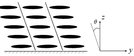
[image:9.612.181.425.224.425.2]0.2 0.4 0.6 0.8 1.0 1.2 1.4 1.6 1.8 2.0
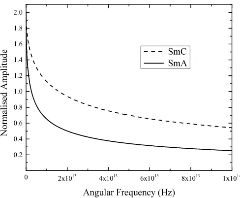
Figure 4: The amplitudes |C|SmA and |C|SmC of the refracted waves, normalised with respect toA. Note that both continuum theories predict the same qualitative behaviour.
Figure 4 displays the behaviour of the amplitudes in both the SmA and SmC, i.e. |C|SmA
and |C|SmC, as functions of the incident angular frequency ω. Parameter values for SmC were
taken from [12, p. 301] where we have set τ5 −τ1 > 0, λ5 −λ2 > 0 and θ = π/6. The values for SmA were obtained from Table 1 in reference [15]; for the solid, we chose ρs = 2400kgm−3 and µs = 2.62×10¹⁰Pa. Clearly the behaviour of each of these expressions in (5.3) and (5.5) is qualitatively the same, and we observe that, untilω∼1010Hz,
|C|SmA ∼ 2−1.01×10
−6√ω
A, (5.6)
|C|SmC∼ 2−4.12×10
−7√ω
A, (5.7)
from which it is evident that|C|SmA +1.9A and |C|SmC +1.96A when ω = 1010Hz, both showing
comparatively little change over the range 0 ≤ ω . 1010Hz. Thereafter, the refracted wave am-plitudes begin to fall off more noticeably, and byω = 1014Hz, |C|SmA is just over one tenth of its
initial value, while|C|SmC is somewhat below thirty percent of its initial value.
6
Discussion
and refracted waves in terms of the problem’s physical parameters. In particular, the refracted wave numberq, which characterises the attenuation of the wave in the SmA case, was provided in terms of the parameters characterising the solid and the smectic by equation (3.16). Further, expressions for the amplitudes of these at normal incidence were derived in terms of the incident wave amplitude and these parameters, with (5.2) and (5.3), lead to expressions for the reflected and refracted waves, respectively. For the purpose of a qualitative comparison, we derived analogous terms via the results of Gill and Leslie [2], who performed calculations for the identical experiment for a sample of SmC, utilising the LSN theory for SmC. It is readily seen that, at normal incidence, the behaviour of the two phases is qualitatively the same, with the refracted wave amplitudes showing a departure in behaviour from the approximate expressions given in equations (5.6) and (5.7) asωincreases beyond the critical value 1010Hz. Beforeωattains this value, the aforementioned expressions provide a very accurate approximation to the respective exact expressions for the refracted wave amplitudes given in (5.3) and (5.5).
The assumption of spatially semi-infinite samples is valid for samples whose depth is greater than that of the penetration depth given in either (4.18) for SmC or (4.19) for SmA in the case of normal incidence. It may prove instructive to consider a smectic confined to a region whose depth is less than that of these penetration depths and investigate the effects of the boundaries in this case. Further, the linear stability of the layered structure to perturbations will presumably be valid for sufficiently small amplitudes of incident wave; just how sensitive the smectic sample is to higher magnitude disturbances is a matter for further investigation.
References
[1] Landau, L. D., Lifshitz, E. M. (1987).Fluid Mechanics, Landau and Lifshitz: Course of The-oretical Physics, Vol. 6, 2nd Ed., Butterowrth-Heinemann: Oxford, UK.
[2] Gill, S. P. A., Leslie, F. M. (1992). J. Mech. Phys. Solids, 40, 1485. [3] Stewart, I. W. (2007).Continuum Mech. Thermodyn., 18, 343.
[4] Auernhammer, G. K., Brand, H. R., Pleiner, H. (2000). Rheol Acta, 39, 215. [5] Auernhammer, G.K., Brand, H.R., Pleiner, H. (2002). Phys. Rev. E, 66, 061707. [6] Ribotta, R., Durand, G. (1977).J. Physique, 38, 179.
[7] Aris, R. (1989). Vectors, Tensors, and the Basic Equations of Fluid Mechanics, Dover: New York, USA.
[8] De Vita, R., Stewart, I. W. (2013).Soft Matter, 9, 2056.
[9] Landau, L. D., Lifshitz, E. M. (1986). Theory of Elasticity, Landau and Lifshitz: Course of Theoretical Physics, Vol. 7, 3rd Ed., Butterowrth-Heinemann: Oxford, UK.
[10] Spencer, A. J. M. (2004).Continuum Mechanics, Dover: New York, USA.
[11] Leslie, F. M., Stewart, I. W., Nakagawa, M. (1991).Mol. Cryst. Liq. Cryst., 198, 443.
[12] Stewart, I.W. (2004). The Static and Dynamic Continuum Theory of Liquid Crystals, Taylor & Francis: London, UK.
[13] Gill, S. P. A. (1992). Ph.D. Thesis, Department of Mathematics, University of Strathclyde, Glasgow.
[14] Miscandlon, J., Stewart, I. W.In preparation.